The Measurement of Poverty with Geographical and Intertemporal Price Dispersion. Evidence from Rwanda

DIAL • 4, rue d’Enghien • 75010 Paris • Téléphone (33) 01 53 24 14 50 • Fax (33) 01 53 24 14 51 E-mail : dial@dial.prd.fr • Site : www.dial.prd.fr

D

OCUMENT DE

T

RAVAIL

DT/2005-16

The Measurement of Poverty with

Geographical and Intertemporal

Price Dispersion

Evidence from Rwanda

THE MEASUREMENT OF POVERTY WITH GEOGRAPHICAL AND

INTERTEMPORAL PRICE DISPERSION

Evidence from Rwanda Christophe Muller2

Departamento de Fundamentos del Análisis Económico Universidad de Alicante

cmuller@merlin.fae.ua.es

Document de travail DIAL Décembre 2005 ABSTRACT

It is not known to what extent welfare measures result from seasonal and geographical price differences rather than from differences in living standards across households. Using data from Rwanda in 1983, we show that the change in mean living standard indicators caused by local and seasonal price deflation is moderately significant at every quarter. By contrast, the differences in poverty measures caused by this deflation can be considerable, for chronic as well as transient or seasonal poverty indicators. Thus, poverty monitoring and anti-poverty targeting can be badly affected by inaccurate deflation of living standard data. Moreover, when measuring seasonal poverty, the deflation based on regional prices instead of local prices only partially corrects for spatial price dispersion. Using annual local prices instead of quarterly local prices only yields a partial deflation, which distorts the measure of poverty fluctuations across seasons and biases estimates of annual and chronic poverty.

Key Words: Measurement and Analysis of Poverty, Income Distribution, Personal Income Distribution.

RESUMÉ

On ne sait pas dans quelle mesure les indicateurs de bien-être social résultent de différences de prix plutôt que de différences saisonnières et géographiques de niveaux de vie entre ménages. A partir de données du Rwanda en 1983, nous montrons que le changement de la mesure du niveau de vie moyen causé par la déflation des prix est modéré bien que significatif à chaque trimestre, contrairement au changement des mesures de la pauvreté qui peut être considérable, que ce soit pour des indices de pauvreté chronique, transitoire ou saisonnière. Ainsi le suivi de la pauvreté et le ciblage anti-pauvreté peuvent être sévèrement affectés par une déflation imprécise des données de niveaux de vie. Pour la mesure de la pauvreté saisonnière, la déflation basée sur des indices de prix régionaux, au lieu d’indices de prix locaux corrige seulement partiellement la dispersion géographique des prix. De même, employer des prix locaux annuels au lieu de prix locaux trimestriels conduit à une déflation partielle qui non seulement distord la mesure des fluctuations de la pauvreté entre les saisons, mais fournit également des estimations biaisées des pauvretés chroniques et annuelles.

Mots clés : Mesure du niveau de vie, Variation spatiales de prix, Mesure de la pauvreté, Politiques de lutte contre la pauvreté

JEL Code: I32, O15, D31

1 _{This is a revised version of the CREDIT Working Paper with the same title. I thank participants in seminars at the University of Oxford,}

INRA-IDEI at Toulouse, STICERD at the London School of Economics, and at the University of Manchester, and at the IARIW conference in Cambridge for their comments, particularly J. McKinnon, J.-P. Azam, C. Scott and F. Cowell. Usual disclaimers apply.

2 _{The author acknowledges a TMR grant from the European Union for starting this paper. I am grateful to the Ministry of Planning of}

Rwanda which provided me with the data, and in which I worked from 1984 to 1988 as a technical adviser from the French Cooperation and Development Ministry. I am also grateful for the financial support by Spanish Ministry of Sciences and Technology. Project No. BEC2002-03097 and and by the Instituto Valenciano de Investigaciones Economicas.

Contents

INTRODUCTION ... 4

1. POVERTY MEASURES AND PRICE INDICES... 5

1.1. Price indices and living standards... 5

1.2.Poverty measures... 6

1.3.Estimators ... 6

2. THE DATA ... 7

2.1.Consumption data ... 7

2.2.Price data... 8

3. WELFARE ESTIMATION RESULTS... 10

3.1.Mean living standards by quintiles ... 10

3.2.Poverty estimates ... 11

3.3.Variation in the definition of the poor ... 13

4. USING LOCAL OR REGIONAL PRICES? ... 13

4.1.Statistical tests and estimates... 13

4.2.Measurement and sampling errors on prices... 14

CONCLUSION... 16

APPENDICES ... 17

BIBLIOGRAPHY ... 20

List of tables

Table 2: Percentages of variation of mean per capita consumption ... 10

Table 3: Proportion of changes in FGT(0) and FGT(2) poverty measures due to local and seasonal price deflation... 12

Table 4: Variation in the population of the poor caused by the deflation (%) ... 13

Table 5 a: Regional seasonal mean prices (Frw) ... 15

Table 5 b: Comparison of local and regional deflations ... 15

List of figures

INTRODUCTION

The design of policies against poverty (see World Bank 1990, 2000) calls for precise measurement of household living standards (Atkinson, 1987; Lipton and Ravallion,1993; Ravallion, 1994). This is all the more difficult in LDCs (Less Developed Countries) because, owing to the high seasonal variability of agricultural output in poor agrarian economies and to the presence of liquidity constraints, prices and living standards of peasants considerably fluctuate across seasons. Another difficulty arises from substantial variations in prices across regions and even across neighbouring areas, because of high transport and transaction costs as well as deficient information (in Indonesia in Ravallion and Bidani, 1994).

The treatment of geographical and temporal price dispersions is crucial for welfare analysis. This has been recognized in LDCs and also for poverty measurement in the U.S. (Citro and Michael, 1995, 2000; The Camberra Group, 2000; Blaise and Sosulki, 2002). Indeed, if the correction for differences in prices that distinct households face at separate periods is inaccurate, then apparent welfare fluctuations, or welfare differences between households, might mostly result from unaccounted price differences. In that situation, household living standards could be more stable or heterogeneous, or the opposite, than they appear to be.

The correction for price differences is generally implemented by deflating the living standard indicator with a price index. Theoretically, price indices could be ratios of cost functions representing consumers’ preferences (Muellbauer, 1974; Glewwe, 1990). In practice, they are usually Laspeyres or Paasche price indices.

Despite this common practice, to our knowledge no statistical analysis of the impact on poverty analysis of price deflation involving local and seasonal prices is present in the literature. In cross-section poverty measurement, some authors use aggregate Laspeyres and Paasche indices based on regional prices (Grootaert and Kanbur, 1994-1996; Dercon and Krishnan, 1998; Jalan and Ravallion, 1998; Appleton, 2000; Kakwani and Hill, 2002). In some instances, it has been noticed, even if without statistical tests, that using different formulations of such indices can yield different poverty levels (Grootaert and Kanbur, 1994). In other cases, using different price indices does not deliver very different poverty rates (Slesnick, 1993). We suspect that in several poverty studies, notably in some analyses of the World Bank’s Living Standard Measurement Surveys, deflation using local prices might have been implemented without attention being specifically drawn to this when writing up the reports3_{. Moreover, the used deflators in this case are based on unit-values rather than} market prices (Deaton and Tarozzi, 2000). This may be a problem if the unit-values incorporate large quality effects that should not appear in price indices. Meanwhile, the norm is still to deflate at very high levels of aggregation. In any case, the impact on poverty of this deflation has not been statistically analysed, and this is our objective in this paper.

Ideally, the deflation of living standards should account for all price differences. Indeed, inflation on the one hand and geographical price dispersions for different products and for the general level of prices on the other hand are often positively correlated, but only weakly (Glezakos and Nugent, 1986; Danziger, 1987; Domberger, 1987; Tang and Wang, 1993). Then, all aspects of price dispersion need to be considered. Finally, some goods are characterised by larger price fluctuations than others, with these fluctuations having a substantial local and seasonal component (Riley, 1961). All this suggests deflating with local price indices incorporating the local movements of specific prices rather than with national inflation indicators. It also implies accounting for the seasonal dispersion of prices as well as annual price variations.

3 _{In some internal documents of The World Bank that cannot be cited due to administrative rules, log-price equations have been estimated}

showing whether local prices can be considered as different from regional prices. Although this approach provides hints about the likelihood of local price effects in poverty analyses, it is different from testing that price effects are significant for poverty measurement.

This is important because price fluctuations have implications for welfare analysis (Baris and Couty, 1981; Jazairy, Alamgir and Panuccio, 1992). However, scant attention has been paid to the role of price dispersion in the measurement of poverty fluctuations. The treatment of price dispersion in studies of living standards fluctuations sometimes refers to a standard national inflation index (Rodgers and Rodgers, 1993; Slesnick, 1993; Deaton, 1999) or is not indicated (Bane and Elwood, 1986; Stevens, 1994; Jalan and Ravallion, 1998).

To study the impact of accurate deflation for welfare analysis, we use data from Rwanda in 1983. This case is interesting in that because Rwanda is small with relatively weak climatic seasonal fluctuations, spatial and seasonal price dispersions may be lower than in many agricultural LDCs, which are often larger and subject to more extreme climatic shocks.

How important is spatial and temporal price deflation for measuring aggregate living standards and aggregate poverty? Can we find systematic effects of accurate price deflation on poverty indicators? Is the correction with regional price indices or with annual prices sufficient to account for prices? The aim of this article is to answer these questions by studying the effects of the price deflation on quarterly, transient and chronic poverty indicators using data from Rwanda. In Section 1, we define poverty measures and price indices and we present poverty estimators. In Section 2, we describe the data used in the estimation. In Section 3, we discuss the estimation and test results. In Section 4, we conduct a comparison of poverty measures deflated respectively using local and regional price indices. Finally, we conclude in Section 5.

1.

1.1.

Laspeyres or Paasche price indices will be our benchmark because we want to assess the impact of price correction carried out in most public offices where they are used. Substitution effects could be important, although they are not incorporated in the analysis because we want to focus on a single issue.

We consider the information available in a household consumption survey and a price survey for each quarter of the same agricultural year. Typically, a household survey collection is organised around local clusters of households. The Laspeyres price index (Ist) specific to a household s and a quarter t, in

which the comparison basis is the annual national mean consumption, is defined as Ist = Σg Sg pgst / pg..

where Sg = (ΣsΣt wst pgst qgst)/(ΣuΣsΣt wst pgst qgst ) is the weight of good g in the price index; wst is the

sampling weight of household s at quarter t, corrected for missing values; pstg is the price of good g in

the cluster where household s is observed. We assume that prices are constant in the same cluster. qgst

is the consumed quantity of good g by household s at quarter t4. The annual national price of good g that is used in the previous definition is:

pg.. = (Σs Σt qgst pgst wst)/(Σs Σt wst). Prices in the above equations are weighed both by sampling

weights and consumption quantities. Indeed, Ist is a Laspeyres price index for which the weight is the

share of consumption value at the national level, consistently estimated by Sg. On the other hand, p..g is

a consistent estimate of the mean price for all consumed quantities of good g at the national level during the year.

We simultaneously consider the quarterly and geographical dispersions of prices. Other approaches would be to focus (1) on the geographical dispersion by choosing the price basis as a national average of the prices for each considered quarter; or (2) on the aggregate seasonal dispersion of prices by choosing the price basis as a yearly local average. However, these approaches would only pick up part

4 One could also consider a Paasche price index (as in Deaton and Zaidi, 1999). However, to avoid mixing too many issues we focus on the Laspeyres price index in this paper. Trials with a Paasche index have exhibited the same qualitative impact of the spatial distribution of prices than with the Laspeyres index.

of the error made when not correcting for price differences. The next sub-section shows how living standards are incorporated in poverty measures.

1.2.

The living standard indicator for household s at quarter t is yst = cst/(E.Ist ) where cst is the value of

consumption of household s at quarter t, E is the household size (or an other equivalence scale). The non-deflated living standard indicator is denoted nominal living standard. The average living standard of household s over the studied agricultural year is denoted average living standard. Because of the short observation period we neglect discount factors between quarters.

We now present notions of quarterly poverty, chronic poverty and transient poverty. The names for poverty indices (‘chronic’, ‘transient’) are of different origin than that for living standards since they come from past poverty studies (Ravallion, 1988; Rodgers and Rodgers, 1993; Jalan and Ravallion, 1998). Pt is the poverty measure calculated in quarter t using the observations yst for all

households. It is denoted quarterly poverty at quarter t. We denote annual poverty the arithmetic mean of the quarterly poverty measures: AP = (P1 + P2 + P3 + P4)/4. The chronic poverty, CP, is the

poverty measure formula applied to the average living standard. It is the poverty indicator that one would want to measure if people could have smoothed consumption if desired.

The transient poverty over the year is the residual of the annual poverty once the chronic poverty has been accounted for: TP = AP – CP. Thus, TP is the poverty increase attributed to the variability of living standards during the year. To stress the fact that TP comes from the seasonal fluctuations of living standards, we denote it transient-seasonal poverty. Indicators CP and TP have been defined in Ravallion (1988) for annual fluctuations of living standards. Using these approaches, Muller (2003) shows that in Rwanda most of the annual poverty comes from the transient-seasonal component. Note that strictly speaking, chronic poverty does not generally correspond to the permanent household income and transient poverty does not correspond to the deviation of consumption with respect to a normal state. Indeed, households are generally not observed at each quarter with a level of quarterly consumption corresponding to chronic poverty. Also, a given household can be chronically poor and transiently poor at the same time (Baulch and Hoddinot, 2000). We now turn to the estimators of the poverty measures.

1.3.

The usual applied poverty measures in quarter t can be written as Pt = ∫ k(yt, z) dF (yt), where k is the

poverty function describing the poverty severity for living standard yt with poverty line z, and F is the

cdf of living standards in quarter t. The poverty indicators used in the application are described in Section 4.2. The estimator of the poverty measure at quarter t is

(Σn

s=1 wst k(yst, z))/(Σns=1 wst), where wst is the sampling weight of household s at quarter t (s = 1,...,n).

The estimators for AP, CP and TP follow the same logic. The estimator for the variations of poverty measures are obtained by replacing in the formula the poverty function by its variation. The estimator for the sampling standard errors is shown in Appendix 1.

We do not consider sampling errors and measurement errors in the price index (as in Wilkerson, 1966, and White, 1999), despite our acknowledgement of the potential cost of price noise. There are several reasons for this. Firstly, we do not have precise information about these errors. The price indicators were produced by combinations of “expert choices” by the enumerators and the analyst, and complex statistical decisions based on temporal and geographical aggregation (Muller, 2005). A non-tractable sampling scheme for price observations would be necessary to model it. Moreover, the basic price data is no longer available and we cannot estimate standard errors of prices. Then, complete inference incorporating the two sources of sampling errors is impossible. Beyond the data availability issue, there is an additional difficulty: the two sampling processes are likely not to be independent. Indeed, price information is generally collected in locations close to where household live. Then, standard errors in prices and in household consumption would be insufficient for the analysis. Instead, a

complex set of correlation estimates for household and price sampling is necessary. Such complexity is beyond the scope of this paper and the data availability.

Secondly, our intention in this paper is to focus on simple comparisons of poverty indicators, assuming that the source of the differences is the price deflation and that the main error stems from the sampling process for the consumption observations and not from errors in prices. We provide further arguments for this approach in Sub-section 5.2. Wilkerson (1969) find the sampling error of prices in the U.S. CPI has a very low impact on the price index uncertainty: a 0.2 percent change in CPI is significant. In his case, the sampling error mostly comes from collecting price information from various outlets, while the other sources of errors are less important. This evidence, although far from the case of poverty in Rwanda, is encouraging. Note that there does not exist in the literature simultaneous estimations of standard errors for households sampling and price sampling. We now examine the data used in the application.

2.

2.1.

Rwanda in 1983 is one of the poorest countries in the world, with per capita GNP of US $ 270 per annum. More than 95% of the population live in rural areas (Bureau National du Recensement, 1984). Data for the estimation is taken from the Rwandan national budget-consumption survey conducted in the rural part of the country from November 1982 to December 19835_{. 270 households were surveyed} about their consumption. Because of missing values only 265 observations are used in the analysis. The collection of the consumption and price data was organised in four rounds corresponding to quarters: round A from 01/11/1982 until 16/01/1983; round B from 29/01/1983 until 01/05/1983; round C from 08/05/1983 until 07/08/1983; round D from 14/08/1983 until 13/11/1983.

The sampling scheme has four sampling levels: communes, sectors, districts and households (Roy, 1984). The drawing of the communes was stratified by prefectures, agro-climatic regions and altitude zones. Several sectors were drawn in each commune. One district was drawn in each sector and one cluster of three neighbouring households was drawn in each district. From this information, we have calculated sampling weights that are the inverse of the household drawings probabilities. Small measurement errors in consumption are required to study price effects in welfare measurement. Particularly when looking at poverty change over periods, one wants to ascertain that the measured change of living standards is not mostly due to measurement errors. Then, additional changes caused by price correction would appear as genuine. Fortunately, the consumption indicators are of a very high quality because of the intensity of the collection (every household was visited daily during two weeks at every quarter, all food was weighed) and a thorough cleaning of the data under our supervision based on sophisticated verification algorithms.

The observed seasonal fluctuations of consumption and prices can be considered typical. Since the agricultural year 1982-83 is a fairly normal climatic year6_{. It is also preserved from extreme economic} or political shocks. The agricultural year includes two growing seasons. The first one extends from October (seeding) to January (harvest), and is dominated by the cultivation of pulses, mostly beans, and to a less extent of corn. The second growing season, during which cereals, mostly sorghum, are cultivated, is from March (seeding) to July (harvest). On the whole, the harvests start at the end of December to finish in April, then from June to July. Meanwhile, Sweet potatoes are harvested at the end of February and the beginning of March, in May, September and end of November. The fourth round is therefore a period with limited harvest. However, cassava and banana cropping are spread across the year, making it difficult to associate with a specific season. Such difficulty is general.

5 _{Ministère du Plan (1986a). The main part of the collection was funded by the French Cooperation and Development Ministry and}

designed with the help of INSEE (French national statistical institute). The author was himself involved in this project as an expert from the French Ministry of Cooperation and Development.

Indeed, an aggregated picture of seasonal agricultural activities does not accurately account for the extreme variety of mountainous agricultural contexts in Rwanda.

Rwanda is characterised by a strong pressure on land (André and Platteau, 1998), with only an average of 1.24 ha of cultivated land for mean household size of 5.22 members. This land yields in real terms a mean production of 57,158 Frw (Rwandan Francs7_{) of agricultural output, close to the value of} average consumption (51,176 Frw or 10,613 Frw per capita). We discuss the price data in the next sub-section.

2.2.

Studies from price surveys in Rwanda reveal substantial geographical and seasonal price dispersions8_. They also provide evidence of intra-regional price variability, even amongst markets of the same region. Finally, large price volatility has been observed in the local production area at the time of the harvest, as opposed to smaller amplitude of variation outside the area (Gabriel, 1974).

These price dispersion features are attributed to transport and stock difficulties and to speculation. Gabriel also mentions temporary shortages in markets. In small markets, the local peasants sell their products and the buyer is often a small trader. In larger markets these small traders can sell to large traders who cover most of the country with their trade. In all cases, consumers are also present. The heterogeneity of these agents, disposing of different information, is another source of inter-regional and intra-regional variability in prices.

To account for these dispersions, we have constructed a price database from the same household survey and an accompanying price survey (See Appendix 3). The incorporation of admissible mean prices in the database not only relies on statistical criteria such as the price sample size9_{, but also on} the expertise of enumerators and analysts. Appendix 2 discusses these price samples.

From this database we obtain our final price indicators by comparing market prices, consumption

prices and production prices at different geographical and temporal aggregation levels for every good.

At each stage of the algorithm of calculus of the price indicators, we control for the representativity of means of recorded prices and for measurement errors so as to select the best price indicators. We discuss in Appendix 3 how these price indicators are calculated.

The prices of each category of goods are represented by the price of the main product in the category. This allows the comparability of prices across seasons and clusters with little quality bias, since this main product remains the same for every sector. Naturally, the quality of the main product may still differ. Missing values of the mean prices of these representative products have been replaced as described in Appendix 3. We are ready to examine some price statistics.

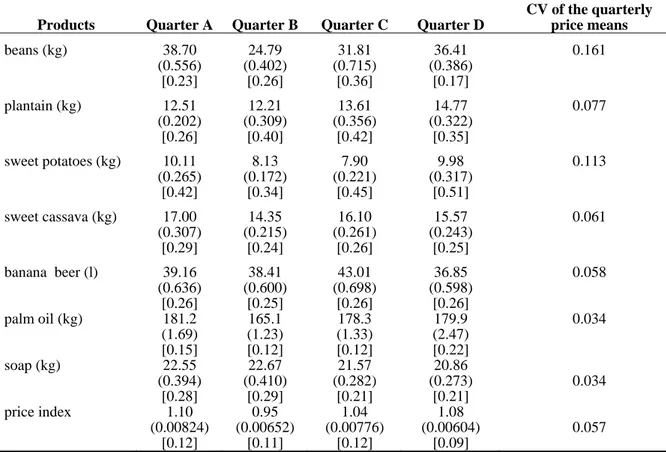
The means and coefficients of variation (CV) of seasonal prices for the main goods used in the price index are shown in Table 1 for the four seasons, together with the price index. Price means at the national level vary with the quarter. The CVs for specific product prices and for the price indicates that the geographical price dispersion is larger than the temporal price dispersion. Then, the aggregate seasonal dispersion of prices cannot properly approximate price differences and hide considerable spatial dispersion. Averaging over products in the calculation of the price indices yields moderate CVs at all quarters, as compared to the CVs for specific products. However, the geographical spread of price indices remains non negligible.

7

In 1983, the average exchange rate was 100,17 Frw for one 1983 US$ (source: IMF, International Finance Statistics), i.e. 60,16 Frw for one 1999 US$.

8 _{Projet Agro-Pastoral de Nyabisindu (1985), Niyonteze and Nsengiyumva (1986), O.S.C.E. (1987), Ministère du Plan (1986), Muller}

(1988), Balanga and Loveridge (1988).

Table 1: Local seasonal mean prices (Frw)

Products Quarter A Quarter B Quarter C Quarter D

CV of the quarterly price means beans (kg) 38.70 (0.556) [0.23] 24.79 (0.402) [0.26] 31.81 (0.715) [0.36] 36.41 (0.386) [0.17] 0.161 plantain (kg) 12.51 (0.202) [0.26] 12.21 (0.309) [0.40] 13.61 (0.356) [0.42] 14.77 (0.322) [0.35] 0.077 sweet potatoes (kg) 10.11 (0.265) [0.42] 8.13 (0.172) [0.34] 7.90 (0.221) [0.45] 9.98 (0.317) [0.51] 0.113 sweet cassava (kg) 17.00 (0.307) [0.29] 14.35 (0.215) [0.24] 16.10 (0.261) [0.26] 15.57 (0.243) [0.25] 0.061 banana beer (l) 39.16 (0.636) [0.26] 38.41 (0.600) [0.25] 43.01 (0.698) [0.26] 36.85 (0.598) [0.26] 0.058 palm oil (kg) 181.2 (1.69) [0.15] 165.1 (1.23) [0.12] 178.3 (1.33) [0.12] 179.9 (2.47) [0.22] 0.034 soap (kg) 22.55 (0.394) [0.28] 22.67 (0.410) [0.29] 21.57 (0.282) [0.21] 20.86 (0.273) [0.21] 0.034 price index 1.10 (0.00824) [0.12] 0.95 (0.00652) [0.11] 1.04 (0.00776) [0.12] 1.08 (0.00604) [0.09] 0.057

Spatial coefficient of variation in brackets. Spatial standard errors in parentheses calculated over 256 observations.

There are two groups of products: the ones with high local and seasonal price dispersions and the ones with high local price dispersion only. The average prices of soap and palm oil are characterised by relatively moderate quarterly fluctuations in terms of the CVs of quarterly price means across the four seasons. The seasonal fluctuations of price means are larger for other goods, with the more variable national prices being those of beans and sweet potatoes. In all cases, the standard error of price means, reflecting the sampling from local to national level, are quite small, much smaller than aggregate seasonal variation in prices. The general level of prices, shown by the mean price index across households, is relatively high in quarters A (1.10) and D (1.08), and low in quarter B (0.95). The months before the December-January harvests are those where the highest mean prices are reported (except for banana, banana beer and soap).

Accounting for geographical and temporal price dispersions matters. Figure 1 shows the evolution curves of mean consumption and mean production across quarters, respectively with and without price deflation10_{. The price deflation reveals that consumption and production are particularly low at the last} quarter, while it dampens consumption indicator fluctuations during the remainder of the year. Production and consumption levels are substantially corrected at quarters A and B, when prices are respectively high and low, before and after the December-January harvests. The following section shows the impact of this correction for welfare analysis. We first discuss the estimates of mean living standards, then the estimates of poverty measures and finally the variation in the definition of the poor.

10 _{Production here is deflated by Laspeyres consumption prices with the weights of the average production structure. This is because}

Figure 1: Evolution of consumption and production

3.

3.1.

The living standard variable is the per capita consumption. Using other equivalence scales does not substantially change our qualitative results. Table 2 presents in percentages the ratios (cD – cND)/cND

where cD and cND are respectively the deflated and non-deflated indicators for the means of per capita

consumption. These data are reported for the four quarters, for the global sample and each quintile of the annual per capita consumption11_{. The results of t-tests of comparisons of means}12 _{show that at the} national level, deflated mean living standards in quarters A, B and D are statistically different from non-deflated mean living standards in the same quarters. This is not the case for period C in which the deflation with the price index is not significant (P-value = 0.14).

Table 2: Percentages of variation of mean per capita consumption ((deflated-nondeflated)/nondeflated)

Variable Quarter A Quarter B Quarter C Quarter D

Per capita consumption (all quantiles) 8.91 - 6.03 1.82 6.83

per capita consumption (Q = 1) 12.04 - 4.65 6.02 9.72

per capita consumption (Q = 2) 6.56 - 1.91 5.01 8.58

per capita consumption (Q = 3) 9.92 - 5.47 5.29 8.16

per capita consumption (Q = 4) 7.82 - 5.48 4.93 5.24

per capita consumption (Q = 5) 9.24 - 8.69 - 4.07 5.68

Q denotes the quintile of per capita consumption, respectively deflated and non-deflated.

These features at least partially persist at the quintile level. Within each quintile of the annual real living standard distribution, the effect of deflation is pervasive. The t-tests generally reject the hypothesis of equality of means. Then, the deflation is generally significant for estimating annual and quarterly mean living standards in most quintiles. This is interesting since, most of the time, living

11 _{Means and standard deviations of the per capita consumption are in Muller (2002).} 12 _{See Wang (1971) for the calculus of the P-values of the tests with small sample.}

standards statistics are published non-deflated in the reports of household surveys. Caution seems advisable when interpreting non-deflated results as genuine welfare statistics.

However, the differences in these aggregates, with and without deflation, are moderate, generally below ten percent (on average over all quintiles: 9.1% in quarter A, - 5.2% in B, 3.4% in C, 7.5% in D). Quarter D is unambiguously a hardship period: mean per capita consumption is lower whether measured with or without price deflation. For the first three quarters, these averages evolve more regularly when deflated indicators are used, while the consumption fall is larger at the last quarter with price adjustment. The latter results do not always persist at the quintile level, which indicates that aggregate means might be misleading where fluctuations in living standards are concerned.

Which dimension is the most relevant: geographical or seasonal variability? A variance analysis shows that for both prices and living standards, the geographical variability contributes more to the explanation than the seasonal variability. However, both directions of variability must be considered when one wants to compare with results caused by imperfect deflation for the whole year and the whole country.

Finally, studying a single quarter could be sufficient for some purposes, such as long term tracking of changes over years. However, the estimates in the next section will show that poverty in Rwanda is high at every quarter and all of them must be observed for an accurate picture of poverty.

3.2.

We show results for the Foster-Greer-Thorbecke (FGT) poverty measures (Foster, Greer and Thorbecke, 1984). We focus on FGT(0), that is the head-count index (poverty function: 1[y<z]) and FGT(2), that is the squared poverty gap (poverty function: (1-y/z)2.1[y<z]) accounting for the inequality among the poor. We have found similar results for other axiomatically sound poverty measures: the Watts measure (1968), the CHUC measures (Clark, Hemming and Ulph, 1981, Chakravarty, 1983), FGT(1) and FGT(3), and we omit them13_.

We expect that the square poverty gap indicator, which satisfies the transfer axiom, is more sensitive to price deflation than the count index, which does not satisfy this axiom. In particular, the head-count index should be little sensitive to small errors caused by imperfect deflation when few households are around the poverty line. One may anticipate a relatively lower (respectively higher) measured deflated poverty compared to non-deflated poverty at quarter B (A) where the mean price index is low (high). For all quarters and for the whole year, the size and the direction of the bias are a priori unknown. The following application clarifies this point and confirms the above expectations. Two poverty lines are used. When deflating, we define ZA as the first quintile of annual real living

standards and ZB as the second quintile of annual real living standards. We denote the population

whose per capita consumption is under ZA, the “very poor”, and the population whose per capita

consumption is under ZB as “the poor”. When not deflating, the same lines have been calculated using

the nominal per capita consumption distribution, i.e. ZA (ZB) is the first (second) quintile of the annual

nominal living standard. This implies: (1) the poverty lines are relative to the living standard distribution considered, as is frequently the case in poverty studies; (2) exact chronic incidence of poverty based on FGT(0) should be equal to 20 percent for exactly estimated ZA and 40 percent for ZB,

although seasonal incidence of poverty and other poverty indicators differ from these proportions. In practice, because the estimators may not exactly divide the weighed sample in quintiles, some estimates only non-significantly differ from 20 percent and 40 percent and we omit them in the table. Results for four other poverty lines are similar to the ones presented. We now discuss the estimates based on the above indicators by examining: the statistical significance of the deflation, the sign and the magnitude of the correction, and how it affects the measured share of transient poverty.

13 _{Here, poverty is measured in terms of poor households rather than poor individuals. The alternative approach provides similar results as}

Table 3 shows for FGT(0) and FGT(2) estimates based on poverty lines ZA and ZB the percentage of

variation, ∆Pt/Pt, where ∆Pt is the variation of Pt induced by the deflation. Since the commented

variations are variations in poverty indicators but not in poverty itself, the non-significance must be tested. The estimates of sampling standard errors (shown in Muller, 1999) show that only certain variations are significant. Systematic non-significant differences would imply that the price deflation is useless. This is not the case. Surveys with larger samples should produce more significant differences, reinforcing our results.

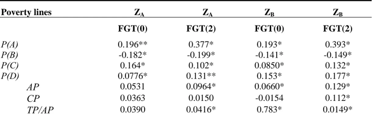
Table 3: Proportion of changes in FGT(0) and FGT(2) poverty measures due to local and seasonal price deflation

Poverty lines ZA ZA ZB ZB FGT(0) FGT(2) FGT(0) FGT(2) P(A) 0.196** 0.377* 0.193* 0.393* P(B) -0.182* -0.199* -0.141* -0.149* P(C) 0.164* 0.102* 0.0850* 0.132* P(D) 0.0776* 0.131** 0.153* 0.177* AP 0.0531 0.0964* 0.0660* 0.129* CP 0.0363 0.0150 -0.0154 0.112* TP/AP 0.0390 0.0416* 0.783* 0.0149*

The numbers shown are: (poverty estimates deflated by local price indices)/(non-deflated poverty estimates)-1, i.e. the proportionate effects of the deflation. Sampling standard errors for the differences are available in Muller (1999). *= difference significant at 5 % level. ** = difference significant at 10 % level.

FGT(0) is the head-count index and FGT(2) is the squared poverty gap. P(A), P(B), P(C), P(D) denote the poverty measures for the successive quarters A, B, C, D of the agricultural year. AP is the annual poverty = (P(A)+P(B)+P(C)+P(D)/4. CP is the chronic poverty. TP is the transient poverty.ZA is the poverty line equal to the first quintile of the annual per capita consumption (with or without deflation). ZB is

the poverty line equal to the second quintile of the annual per capita consumption (with or without deflation). As mentioned in the text, changes in FGT(0) should be zero if the distributions and the poverty lines were perfectly known instead of estimated. Here, they are insignificant even at 10 percent level.

With these poverty lines, the price deflation brings significant changes in poverty measures: a 10 percent change is not uncommon. For CP based on FGT(2), systematically significant results for changes are found with the upper (poverty) line, but not with the lower line. Changes in AP are significant at 5 percent level for both poverty measures with the upper line, but only for FGT(2) when using the lower line. Moreover, the deflation significantly affects quarterly poverty indicators at all quarters. Its impact is major at quarters A and B, in which the aggregate level of prices is well apart the yearly average. The variations in TP are statistically significant except for poverty incidence with the lower line. On the whole, even with a small sample, the local deflation is frequently significant for the two poverty lines, all poverty indicators and most quarters. This result is robust to using other poverty lines and other poverty indicators. Let us turn to the sign of the correction.

The sign of ∆Pt is positive, except in quarter B where the aggregate price index is high and ∆Pt is

negative. However, we have checked with a larger set of poverty lines that this sign cannot be systematically inferred, except in periods of large aggregate price movements (quarters A and B). In part, this is due to the change in the line accompanying the price deflation. The estimates are nonetheless often consistent with a dominance of the effects of the aggregate price shifts across quarters.

The absolute magnitude of changes in poverty measures is considerable, notably for seasonal poverty in quarters A and B. However, this is not systematic and depends on the poverty line and poverty indicator. The magnitude of changes in CP varies a lot (from –1.5 to 11.2 percent). The magnitude of changes in PA (19 to 39 percent) and in PB (-19 to -14 percent) is also substantial. The magnitude of

changes in PC (8 to 16 percent) and PD (7 to 18 percent) is smaller but still non negligible. When

considering other lines, it appears that the impact of the deflation depends much on the line, although it is generally sizeable. As expected, the relative changes caused by the deflation are larger in absolute value with the squared poverty gap than with the head-count index. This is observed for AP, CP and quarterly poverty indicators.

Transient poverty is underestimated when not deflating. The change in the measured share of transient poverty can sometimes be considerable (78 percent for the head-count index and the lower line),

although it is generally small (about 5 percent). Non-deflated price dispersion hides part of the influence of the seasonality of living standards on annual poverty. This is consistent with the fact that at seasons with low agricultural output, living standards are low and food prices are high, and the opposite when output is high. We now look at the consequences of the deflation for anti-poverty targeting.

3.3.

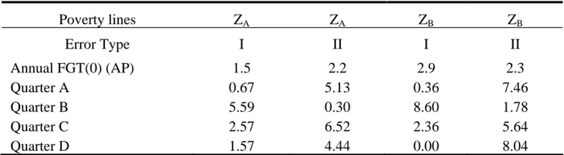
The deflation may change the measured composition of the population of the poor even when the aggregate poverty measure is not significantly modified. In Table 4, the percentages of households that are considered poor before the deflation but not after, are shown in columns ‘Type I error’ (for ‘false poor’). Columns ‘Type II error’ (for ‘omitted poor’) show the percentages of households that are considered poor after the deflation but not before. For policy targeting, Type II is sometimes considered more important since some needy households cannot be reached at all.

The size of changes in the definition of the poor that is caused by the deflation varies. On the whole, Type I errors dominate. However, at the quarterly level substantial changes in the definition of the poor can arise from both incorporating and eliminating households. The pattern of changes in the poor population is affected by the aggregate shift of the price index, although it is not sufficient to explain it. In quarter A when the aggregate price index is high before January harvest, the Type II errors are more numerous than the Type I errors, while it is the opposite in quarter B. These results, which have been found for a larger set of lines, correspond to general underestimation or overestimation of poverty, depending on the level of the aggregate price index. In contrast, when comparing the two error types for quarters C and D with an extended set of lines, no strong systematic tendencies appear. Higher percentages of misclassified households are generally observed with higher lines, which is consistent with a larger proportion of the poor in the population14_{. In the next section we compare} results obtained by using local and regional prices.

Table 4: Variation in the population of the poor caused by the deflation (%)

Poverty lines ZA ZA ZB ZB Error Type I II I II Annual FGT(0) (AP) 1.5 2.2 2.9 2.3 Quarter A 0.67 5.13 0.36 7.46 Quarter B 5.59 0.30 8.60 1.78 Quarter C 2.57 6.52 2.36 5.64 Quarter D 1.57 4.44 0.00 8.04

The first column (Type I error) for each poverty line shows the percentage of households that are poor before the deflation and not after. The second column (Type II error) for each poverty line shows the percentage households that are poor after the deflation and not before. ZA is the poverty line equal to the first quintile of the annual per capita consumption (with or without deflation). ZB is the poverty line equal

to the second quintile of the annual per capita consumption (with or without deflation).

As mentioned in the text, changes in chronic FGT(0) should be exactly zero if the distributions and the poverty lines were perfectly known instead of estimated. Here, they are insignificant even at 10 percent level and not shown.

4.

4.1.

Regional price deflators, often used for welfare analysis, are not likely to introduce distortions caused by quality choices as with local prices computed on household budget data. Since Rwanda is divided in five agricultural regions (Northwest, Southwest, Centrenorth, Centresouth, and East), the regional price indices are defined as the mean price indices over each region. T-tests results show that the

14 _{Unfortunately, the small sample size does not allow to study the characteristics of the poor that would have been overlooked when not}

regional mean price index means significantly differ across regions and quarters, from 0,889 at quarter B in the East through 1,139 at quarter A in the Centrenorth.

They also show that regional price variation is generally significant for specific goods. This occurs for all quarters and all representative products and the regional price means are sometimes far apart. Regional differences are less marked for banana beer, palm oil and soap, widely traded throughout the country. The standard deviations of the product prices indicate that intra-regional price dispersion at the same quarter is not negligible.

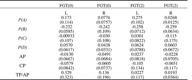
Tables 5b shows the means and standard deviations of the relative variation in poverty measures FGT(0) and FGT(2) induced respectively by local and regional deflations, calculated by considering six poverty lines altogether15_{. It is a way of concentrating six tables specific to each poverty lines into} one. Regional prices only partially correct for the global price dispersion. Poverty estimates with regional deflation are often intermediate between, on the one hand poverty estimates with local deflation, and on the other hand non-deflated poverty estimates. However, the size of the correction with regional prices is also sometimes larger in absolute value than that of the correction with local prices. This cannot be attributed to insignificant deviations since it occurs in particular at quarter B in which deviations are always substantial and significant. In all cases, the differences in the results with the two deflations are frequently considerable, which should induce analysts to prefer local price deflation.

4.2.

There may be considerable noise in price data, which would be an argument favouring the use of aggregate price averages. Using local seasonal price means could introduce additional noise, as compared to national or regional price means, and could outweigh the benefit of high accuracy. However, this is unlikely to explain most of intra-regional price differences since different price surveys in this country indicate similar kind of intra-regional price dispersion. In particular, differences in prices for neighbouring markets have been observed related to local agricultural output supplies, which denotes a genuine empirical basis for the dispersion (P.A.P. Nyabisindu, 1985).

It is also doubtful if the survey sampling errors cause the observed intra-regional price differences because prices were simultaneously collected from a market survey and turned out to be very close to consumption prices (unit-values calculated from records of consumption purchases). This implies that the price differences across households cannot be mostly attributed to random variations coming from the sampling of households. Indeed, the market prices are not subject to the same variations.

The differences between the results with local and regional deflators might also come from the larger size of the price samples used for regional price indices as compared to local price indices, inducing a larger random variability of local price indicators. However, we believe that this is not likely to drive the results because of the above arguments. Moreover, the prices used in local price indices are themselves means of local price samples with a requirement of minimal sample size, which should eliminate some of the non-systematic ‘noise’, although we lack the standard errors to confirm it. Besides, the standard errors of the regional price means in Table 5a show that the corresponding confidence intervals at 5 percent level sometimes overlap for price means in different regions or at different quarters. This result shows that moving from local to regional means is unlikely to eliminate the noise in the data. As a matter of fact, even without noise on local prices (our hypothesis in the calculation of these sampling errors), aggregating to region may add noise to the economically relevant price level that is the local one. All this raises doubts on the usefulness of regional price means.

15

The six poverty lines are defined as follows. z1 is the first quintile of annual living standards; z2 is the sum of the first quintiles of

quarterly living standards; z3 _{is four times the minimum of the first quintiles of quarterly living standards. z}

4 is the second quintile of

annual living standards; z5 is the sum of the second quintiles of quarterly living standards; z6 is four times the minimum of the second

quintiles of quarterly living standards. The same types of poverty lines have been calculated using the nominal per capita consumption distribution (non-deflated). This implies that the lines are relative to the living standards distribution considered.

Table 5 a: Regional seasonal mean prices (Frw) A B C D Northwest (37 obs.) 1.105 (0.0107) 0.951 (0.0106) 1.077 (0.0232) 1.077 (0.0172) Southwest (41 obs.), 1.075 (0.0198) 0.983 (0.0116) 0.960 (0.0156) 1.084 (0.0139) Centrenorth (51 obs.), 1.139 (0.0157) 0.942 (0.0120) 1.098 (0.0135) 1.044 (0.00927) Centresouth (64 obs.) 1.034 (0.00958) 1.006 (0.0114) 1.115 (0.00805) 1.131 (0.00996) East (63 obs.). 1.182 (0.01902) 0.889 (0.0137) 0.976 (0.0177) 1.073 (0.0139)

Spatial standard error in parentheses.

Table 5 b: Comparison of local and regional deflations

FGT(0) FGT(0) FGT(2) FGT(2) L R L R P(A) 0.173 (0.114) 0.0776 (0.0757) 0.275 (0.102) 0.0268 (0.0125) P(B) -0.232 (0.0585) -0.242 (0.109) -0.258 (0.0712) -0.259 (0.0634) P(C) -0.00933 (0.107) -0.030 (0.108) 0.0301 (0.0822) -0.115 (0.175) P(D) 0.0570 (0.0617) 0.0438 (0.0331) 0.0624 (0.0788) 0.0603 (0.0672) AP _(0.0667) -0.0130 _(0.0684) -0.0491 _(0.0818) 0.0237 _(0.0705) -0.0228 CP _(0.0842) -0.0579 _(0.0737) -0.0605 _(0.134) -0.105 -0.0651 _(0.117) TP/AP _(0.323) 0.329 _(0.196) 0.136 _(0.117) 0.0227 _(0.0364) 0.0193

The first number in each cell is the mean of the relative variation caused by the deflation, calculated over six poverty lines. The six poverty lines are defined as follows. z1 is the first quintile of annual living standards; z2 is the sum of the first quintiles of quarterly living standards;

z3 is four times the minimum of the first quintiles of quarterly living standards. z4 is the second quintile of annual living standards; z5 is the

sum of the second quintiles of quarterly living standards; z6 is four times the minimum of the second quintiles of quarterly living standards.

The same types of poverty lines have been calculated using the nominal per capita consumption distribution (non-deflated).

The number in parenthesis is the standard deviation of the relative variation caused by the deflation, calculated over the six poverty lines. FGT(0) is the head-count index and FGT(2) is the squared poverty gap.

Columns (L) correspond to local deflations, while columns (R) correspond to regional deflations.

P(A), P(B), P(C), P(D) denote the poverty measures for the successive quarters A, B, C, D of the agricultural year. AP is the annual

poverty = (P(A)+P(B)+P(C)+P(D)/4. CP is the chronic poverty. TP is the transient poverty.

We now assess the significance of deflation differences by calculating the deviation between the estimates of poverty indices deflated using respectively local and regional price indices (denoted DLR,

for local – regional). Despite the magnitude of the differences in the relative variation caused by the two types of deflation, DLR is not always significant. For CP, DLR is never significant, which suggests

that for poverty indicators corresponding to annual living standards, using regional price indices is sufficient in Rwanda. By contrast at the seasonal level, using local deflation instead of regional deflation is crucial for estimating quarterly poverty in quarters A and C, but not in quarters B and D. Almost all cases where DLR is significant correspond to underestimation of poverty when using

regional prices. This is consistent with a local concentration of the poor in areas far from markets and transaction sites. On the whole, the current practice of developing price deflators only for a few regions is not reliable when studying seasonal poverty, at least in Rwanda, although the bias may be neglected for chronic annual poverty.

Similarly, we investigated the magnitude of the mistake made relative to the difference between quarterly and annual prices (see Muller, 1999, for tables and comment). Here again, we find that using price indicators at the lowest level of aggregation is essential. In particular, the share of transient poverty is biased upward by using annual prices.

CONCLUSION

Static and dynamic welfare indicators are generally imperfectly corrected for price dispersion across households and seasons. To our knowledge, the importance of price correction at local and seasonal level for welfare measurement has not been empirically studied in the literature.

Using seasonal panel data from rural Rwanda, we show the importance of an accurate price deflation based on local and seasonal prices. In many instances, the price deflation significantly changes the measured mean living standards and poverty indicators, whether quarterly, chronic or transient. However, if changes in measured aggregate living standards are moderate in every quarter, this is not always the case for measured poverty, for which the magnitude of changes can be considerable. The structure of welfare changes is also affected by the deflation. Mean living standards and poverty measures appear to vary more smoothly along the year when based on accurately deflated living standards, but then they also show better the severe welfare crisis after the dry season in Rwanda. In terms of the impact of price deflation on poverty assessment, the choice of the poverty line and the considered quarter are generally more influential than the choice of the poverty indicator. At some quarters the effects of aggregate seasonal fluctuations of prices can dominate the effect of geographical price dispersion to imply substantial and unambiguously positive or negative variations of poverty measures in these periods when deflation is implemented. Poverty indicators stressing on poverty severity are more likely to deliver powerful deflation effects. Moreover, the deflation modifies the composition of the population of the poor and therefore affects anti-poverty targeting.

The comparison with poverty indicators deflated using regional price indices instead of local price indices shows that when studying seasonal poverty, regional price indices provide an imperfect correction only. If the bias caused by using regional prices is minor for the measurement of chronic and annual poverty in Rwanda, it is not the case when estimating quarterly poverty. Similarly, using annual prices instead of quarterly prices produces not only severely biased measures of seasonal and transient poverty, but also underestimates annual and chronic poverty. Using regional and annual prices is just not good enough for accurate poverty analysis in Rwanda.

When is accurate deflation needed from a policy perspective? Our results suggest that in contrast with the common practice of using regional or annual price correction, detailed price statistics are important in monitoring of policies against poverty. They are particularly useful for guiding first, policies against seasonal and transient poverty since seasonal and transient poverty measures are more sensitive to deflation; second, policies directed against poverty severity as opposed to policies only aiming at reducing the number of the poor. Meanwhile, the impact of the deflation on measured mean living standards and the sensitivity of results to the choice of the poverty line show that growth policies and aggregate demand policies addressing problems at different levels of the living standard distribution would be better served by living standard statistics that are accurately deflated.

To fully understand why the results are the way they are, and how the characteristics of Rwanda influence the misleading picture of poverty obtained when not properly deflating, we would need a complete explanation of seasonal and geographical distribution of prices in Rwanda and of its links with the living standard distribution across seasons. Also, our results are based on a particular country at a specific period. Clearly, they show that in that case accurate geographical and temporal deflation is necessary to robust welfare analysis. However, more studies would be necessary to (1) elucidate the precise economic mechanisms involved; and (2) generalise the findings to other countries and periods. Also, more sophisticated price indices anchored on utility levels could be considered, although it is not at the moment common practice in LDCs.

APPENDICES

APPENDIX 1: Sampling standard-error estimators

The complexity of the actual sampling scheme does not allow us a robust use of classical sampling variance formula. We use an estimator for sampling standard errors that is a combination of ‘linearization’ estimators obtained using balanced repeated replications (Krewski and Rao, 1981, Roy, 1984, Shao and Rao, 1993) and that is simpler and quicker than stratified bootstrap procedures. Howes and Lanjouw (1998) have shown that the sampling design can modify the estimated standard errors for poverty measures. Consequently, our estimators for the sampling standard errors account for the sample design. Note also that because deflated and non-deflated welfare measures are based on the same sample of observations, their difference, which is the difference of a mean over the same sample, is equal to the mean of the difference over this sample. Then, tests of the difference are simply tests of this significance of this difference and involve similar calculations to the sampling standard errors for the poverty measures.

The poverty indicator of a sub-population is estimated by a ratio of the type

x

z

=

y

′

′

'

where ' denotes the Horwitz-Thompson estimator for a total (sum of values for the variable of interest weighted by the inverse of the inclusion probability). z is the sum of the poverty in the sub-population and x is the size of the sub-population. The variance associated with the sampling error is then approximated by: ) x ( / )] x V( ) y ( + ) x , z Cov( y 2 ) z [V( = ) y V( 2 2 x x x ′ − ' ′ ′ ' ′ ′ '

obtained from a Taylor expansion at the first order from function Y = f(Z/X) around (E y', Ex' ) and because E z' ≠ 0 and x' does not cancel, where the appropriate expectations are estimated by x' and

'

y_x.

We divide the sample of communes (first actual stage of the sampling since all the prefectures are drawn) in five super-strata (α = 1 to 5) so as to group together the communes sharing similar characteristics, and to a priori reduce the variance intra-strata. Several sectors are assumed to have been drawn in each strata. This allows the estimation of the variance intra-strata, while the calculation of the variance intra-commune was impossible, since in fact only one sector had been drawn in each commune. Then, the Horwitz-Thompson formula for superstrata α is:

and

z

q

Q

n

N

m

M

=

z

Σ

Σ

Σ

Σ

'

x

q

Q

n

N

m

M

=

x

Σ

Σ

Σ

Σ

'

where Mh is the number of communes in prefecture h; mhα is the number of communes in prefecture h and drawn in superstrata α; Nhi is the number of sectors in commune i of prefecture h and superstrata

α; nhi is the number of sectors drawn in commune i of prefecture h and superstrata α; Qhij is the

number of households in sector j of commune i of prefecture h; qhij is the number of households drawn

in sector j of commune i of prefecture h and superstrata α. Similar formulae can be used to account for the intermediary drawing of one district in every sector.

Cov(z',x') is estimated by:

)

x

).(x

z

(z

20

1

=

)

x

,

z

ov(

C

′

−

′

−

′

′

_Σ

'

'

ˆ

APPENDIX 2: Properties of the elementary price samples

A preliminary analysis of the consumption price means and the market price means has shown that these indicators are very close and cannot be systematically ordered. These two latter types of price indicators have different qualities. Market price surveys are believed to provide price information that is less dependent from household tastes and purchasing power by better controlling quality choices. However, since price observations are collected only in selected sites, they may provide inaccurate estimates of the prices to which are confronted some households. Moreover, the wording of the questions and the whole collection process of prices are always debatable in that they constitute an artificial observation situation, different from what occurs during actual transactions. Finally, it is never possible to obtain price observations for all goods in all selected markets or transaction sites. This means that the treatment of missing values for prices is an important stage of using market price data. Furthermore, even when price observations are available, the analyst is not content to use them if they are isolated. A large sample of price observations is in fact necessary and what is called “market price” in the price data file is a central tendency of this sample, the mean or the median of observed prices.

When budget data are used to calculate prices, the information about prices fits more closely the consumption pattern of the household. Indeed, goods that are usually consumed in an area generally appear in purchase or sale transactions, even when they are only consumed in kind (from their own production or received as gift) by some of the households of this area. Unfortunately, the prices extracted from a budget survey are in fact elementary “unit-values”, i.e. ratios of values over quantity extracted from observations of individual transactions. Elementary unit-values are believed to be affected by quality choices of consumers or sellers. In that situation, a higher level of prices for a specific household might come from a higher quality of its consumption. Moreover, consumption data is known to incorporate large measurement errors that can be amplified by the use of unit-values instead of exogenous prices. Of course, when no price data are available, unit-values Laspeyres indices might well be better than no correction at all.

This problem for elementary goods is much less serious than for unit-values calculated from categories of consumption, as in Deaton (1988, 1990), where similar goods are aggregated in a common category, for example “fish”. In the latter case the unit-value calculated from these aggregate values and quantities has little in common with the observed prices in a market (the price of a specific fish). However, even if one expects it to be here relatively minor with specific goods, the quality choice remains.

APPENDIX 3: Selection of the Price Indicators • Price database

Three types of prices are in the database. First, the consumption prices are mean prices for each commodity, calculated from the records of consumption purchases. The means are weighed by using the sampling scheme and the consumption levels of surveyed households for the considered good as shown above, while at the cluster level instead of the national level. Second, the production prices are mean prices for each product, calculated from the records of household production sales. Here, the means are weighed by using the sampling scheme and the production level of the surveyed households for the considered product. Third, market prices are unweighed means from the price survey in the markets or transaction sites near the location of the surveyed households.

Market prices were collected once every quarter at the middle of the daily interviews of households in a cluster. The collection took place in the closest markets where the surveyed households had declared that they make most of their purchases. The information was obtained by interviews with sellers and weighing of the products. Therefore, the market prices are based on actual values rather than price announcements. Once a sufficient number of prices has been collected among several important sellers in the market, the market price of this product is calculated as the arithmetic mean of these observations after outlier values have been eliminated. Because each household is surveyed daily during two weeks, these prices can be considered as fortnight prices.

Because of the small differences in production prices and consumption prices, market price means and consumption price means at the cluster level are acceptable approximations of shadow prices and are used where possible in the calculus of price indices.

Despite their relative proximity, there are several reasons to use consumption prices and market prices rather than production prices. First, the date of the information present in the questionnaire corresponds better to the actual consumption when using consumption prices or market prices. Indeed, in each sector these prices are collected during the same week as most of the consumption information, while the production prices are calculated from sale transactions often based on quarterly retrospective records. Second, the final consumption of the goods corresponding to the actual observation of consumption prices and market prices is almost contemporary to the price observations, whereas the observed sales on which are based the production prices may sometimes be the object of consumption, only much later, after several trade intermediations, and sometimes out of the considered district. Third, we want to avoid mixing the two types of price means (consumption price and market price means vs. production price means, because of the slightly lower level of production prices). The sample of observations of production prices is much smaller. It is therefore logical to eliminate it to base the analysis on the sample of consumption prices and market prices.

• Replacement of missing values

Firewood has been eliminated from the consumption (2.9 percent of the aggregate consumption), because the corresponding price means are missing in too many clusters. For the other categories the mean price of a representative product is sometimes missing because of infrequent consumption of the product in the considered cluster. This is attributed to penury of the product, the consumption demand fluctuating less than the production supply for seasonal agricultural products. In that case, the price of the product should be higher than usual and we used the larger sector price mean observed in the same region as an approximation.

BIBLIOGRAPHY

André C., Platteau J.-P.( 1998), “Land Relations Under Unbearable Stress: Rwanda Caught in the Malthusian Trap”, Journal of Economic Behaviour & Organization, 34(1), 1-47, February.

Appleton S. (2000), “Changes in Poverty in Uganda, 1992-1997,” in P. Collier, R. Reinnikka (eds.),

Firms, households and government in Uganda's recovery.

Atkinson A.B. (1987) “On the Measurement of Poverty,” Econometrica, Vol. 55-4, 749-764, July. Bane M.J., Ellwood D. (1986), “Slipping Into and Out of Poverty: The Dynamics of Spells”, Journal

of Human Resources, 21(1), 1-23, Winter.

Baris P., Couty P. (1981), “Prix, marchés et circuit commerciaux africains,” Amira, No 35, Décembre. Baulch R., Hoddinot J. (2000), “Economic mobility and poverty dynamics in developing countries”,

Journal of Development Studies, Vol. 36(6), August.

Betson D.M., Citro C.F., Michael R.T. (2000), “Recent Developments for Poverty Measurement in U.S. Official Statistics”, Journal of Official Statistics, Vol. 16-2, 87-111.

Blaine R., Sosulski M. (2002), “Adjusting Thresholds for Geographic Areas”, mimeo Wisconsin University.

Bulletin Climatique du Rwanda (1982, 1983, 1984), Climatologie et Précipitations, Kigali, Rwanda. Bureau National du Recensement (1984), Recensement de la Population du Rwanda, 1978 : Analyse

Tome 1, Kigali, Rwanda.

Bylenga S., S. Loveridge (1988), “Intégration des prix alimentaires au Rwanda, 1970-86”, Note SESA, Kigali, Rwanda.

Chakravarty S.R. (1993), “A New Index of Poverty”, Mathematical Social Science, N°6, 307-313. Citro C.F., Michael R.T. (1995), Measuring Poverty. A New Approach, National Academic Press. Clark S.R., Hemming, Ulph D. (1981), “On Indices for the Measurement of Poverty”, Economic

Journal, N°91, 515-526, June.

Danziger L. (1987), “Inflation, Fixed Cost of Price Adjustment, and Measurement of Relative-Price Variability: Theory and Evidence,” The American Economic Review, Vol. 77-4, 703-710, September.

Deaton A. (1998), “Quality, Quantity, and Spatial Variation of Price,” The American Economic

Review, pp 418-430.

Deaton A. (1990), “Price Elasticities from Survey Data. Extensions and Indonesian Results” Journal

of Econometrics, 44, 281-309.

Deaton A. (1998), “Getting Prices Right: What Should Be Done?”, Journal of Economic Perspective, Vol. 12-1, pp 37-46, Winter.

Deaton A., Tarozzi A., “Prices and Poverty in India”, mimeo Princeton University, July.

Deaton A., Zaidi S. (1999), “Guidelines for Constructing Consumption Aggregates for Welfare Analysis”, mimeo The World Bank.