HAL Id: pastel-00005145
https://pastel.archives-ouvertes.fr/pastel-00005145
Submitted on 20 May 2009HAL is a multi-disciplinary open access archive for the deposit and dissemination of sci-entific research documents, whether they are pub-lished or not. The documents may come from teaching and research institutions in France or abroad, or from public or private research centers.
L’archive ouverte pluridisciplinaire HAL, est destinée au dépôt et à la diffusion de documents scientifiques de niveau recherche, publiés ou non, émanant des établissements d’enseignement et de recherche français ou étrangers, des laboratoires publics ou privés.
Statistical approach to the optimisation of the technical
analysis trading tools: trading bands strategies
Marta Ryazanova Oleksiv
To cite this version:
Marta Ryazanova Oleksiv. Statistical approach to the optimisation of the technical analysis trading tools: trading bands strategies. Humanities and Social Sciences. École Nationale Supérieure des Mines de Paris, 2008. English. �NNT : 2008ENMP1584�. �pastel-00005145�
Statistical Approach to the Optimisation of the
Technical Analysis Trading Tools: Trading
Bands Strategies
Directeur de these: Alain Galli
Jury:
Delphine Lautier Rapporteur Yarema Okhrin Rapporteur Michel Schmitt Examinateur Frederic Philippe Examinateur
Acknowledgment
I want to thank my advisor Alain Galli for all his thoughtful guidance.
Many thanks to the Members of the Jury - Delphine Lautier, Yarema Okhrin, Michel Schmitt and Frederic Philippe for their time and valuable feedback.
I am grateful to Margaret Armstrong for her kind mentoring.
My special thanks go to:
ֵ CERNA staff for giving me this opportunity, which made this research work possible
ֵ professors Maisonneuve, Schmitt and Préteux of Ecole des Mines for their classes in probability theory and stochastic processes
ֵ Matthieu Glachant, my fellow doctoral students and all participants of the research ateliers, for their constructive critiques
ֵ Jerome Olivier and Frederic Philippe of Banque BRED for sharing their business perspectives and providing informational support for certain elements of this thesis that were completed during my project with them.
ֵ Sesaria Ferreira for the great administrative and logistical help.
The five years I spent in Paris working on this thesis were more than just the time of my professional growth - it was a magnificent personal adventure. I thank my dear friends who shared this journey with me: Larysa Dzhankozova, Anne-Gaelle Geffroy, Yann Ménière, Sevdalina and Panayot Vasilev, and Biket and Doga Cagdas.
Many thanks to my parents-in-law, Elena and Yuri Razanau, for always having the words of encouragement in difficult moments.
I am thankful to my husband Aliaksei Razanau for his loving support, and to my son Mark who has been my greatest source of inspiration.
There are no words to fully express my indebtedness to my parents, Tamara and Igor Oleksiv, without whom none of my achievements would have been possible.
Abstract
In this thesis we have proposed several approaches to improve and optimize one of the most popular technical analysis techniques - trading bands strategies. Parts I and II concentrate on the optimization of the components of trading bands: the middle line (in the form of the moving average) and bandlines. Part III is dedicated to the improving of the decision-making process. In Part I we proposed the use of kriging method, a geostatistical approach, for the optimization of the moving average weights. The kriging method allows obtaining optimal estimates that depend on the statistical characteristics of the data rather than on the historical data itself as in the case of the simulation studies. Unlike other linear methods usually used in finance, this method can be applied to both equally spaced data (in our context, traditional time series) and data sampled at unequal intervals of time or other axis variables. Part II proposes a method based on the transformation of the data into a normal variable, which enables the definition of the extreme values and, therefore, the bands’ values, without constraining assumptions about the distribution function of the residuals. Finally, Part III presents the application of disjunctive kriging method, another geostatistical approach, for more informative decision making about the timing and the value of a position. Disjunctive kriging allows estimating the probability of certain thresholds being reached in the future. The results of the analysis prove that the proposed techniques can be incorporated into successful trading strategies.
Cette these propose des approches pour ameliorer et optimiser un des instruments les plus populaire d’analyse techniques – bandes de trading. Les parties I et parties II se concentrent sur l’optimization des composantes des bandes de trading: ligne centrale (representée par la moyenne mobile) et lignes des bandes. La partie III est dédiée à l’amélioration du processus de prise de decision. Dans la partie I on proposes d’utilizer la méthode de krigeage, une approche geostatistique, pour l’optimization des poids des moyennes mobiles. La methode de krigeage permet d’obtenir l’estimateur optimal, qui incorpore les characteristiques statistiques des donnees. Contrarment aux methodes classiques, qui sont utilisées en finance, cette methode peux etre appliquée à deux types des données: echantillonées à distance régulière ou irrégulière. La partie II propose une methode, basée sur la transformation des données en une variable normale, qui permet de definir les valeurs extremes et en consequence les valeurs des bandes sans imposition des contraintes de la fonction de la distribution des residus. Enfin, la partie III presente l’application des methodes de krigeage disjonctif , une autre methode geostatistique, pour les decision plus informative sur le timing et type de position. Le krigeage disjonctif permet d’estimer les probabilités, que certain seuils seront atteints dans le futur. Les resultats d’analyse prouvent que les techniques proposées sont prometeuses et peuvent etre utilisées en pratique.
Resume
L’analyse technique consiste en l’ensemble des instruments, modèles graphiques et règles de trading, qui sont fondées sur la hypothese que les prix passés peuvent être utilisés pour anticiper les prix futurs. Les règles et modèles sont souvent developées par les traders-techniciens. L’analyse technique est largement ignorée par les traders-fondamentalistes, qui définissent leurs stratégies par les valeurs fondamentales (comme des macro- et micro-indicateurs). Ses idées sont aussi rejetées par la majorité de représentants academique, qui n’acceptent pas cette approche comme méthode pour la prevision des prix futurs.
Les chercheurs ont des difficultés pour accepter cette methode pour la raison suivante : L’analyse technique est fondée sur la hypothese que les prix passés peuvent être utilisés pour anticiper les prix futurs. Cette idée contredit l’hypothèse des marchés efficaces (« efficient market hypothesis ») sur laquelle la majorité des modèles financiers classique est basée. L’autre problème avec l’analyse technique est sa nature empirique: les règles de trading sont souvent dérivées d’observations empiriques plutôt que de modèles mathématiques. En plus, c’est plutôt la règle que l’exception pour les traders de déclarer que certains parametres de certaines stratégies sont optimaux sans aucune référence à des conditions, hypothèses et critères d’optimization. Finalement, les barrières linguistiques crées par le jargon et la terminologie technique utilisée par les traders et chercheurs compliquent encore le dialogue entre les deux parties. En conséquence, ce sujet est insuffisamment développé dans les recherches scientifiques, qui évoquent plutot le scepticisme que l’intérêt. Notre
motivation était donc de contribuer à la recherche pour essayer de combler le fossé entre praticiens et scientifiques.
Cette thèse propose des approches pour améliorer et optimiser un des instruments les plus populaires de l’ analyse technique, les bandes de trading. La bande de trading est la ligne placée autour de l’estimateur de tendance centrale. Quatre composantes des bandes peuvent être définis : (1) la série de prix ; (2) la ligne centrale ; (3) la bande haute (supérieure) ; (4) la bande basse (inférieure). Deux types de stratégies peuvent être définis pour cet instrument : (1) « following » ; et (2) « contrariant ». Pour la strategie « trend-following », les bandes servent de confirmations du signal de tendance établi. Au contraire, les bandes définissent les instruments qui sont trop chers ou moins chers pour la strategie « contrariant ». Certainment, les positions prise en contexte de ces types de strategie sont opposées.
Les traders utilisent différents types des bandes. Les classement des bandes peut être défini par les idées/hypothèses conceptuelles en ce qui concerne les prix pour lesquels les bandes sont définies. Par example, les bandes de trading, les plus simples obtenues par le déplacement parallèle de la ligne centrale en haut et en bas, supposent la volatilité constante des prix. Les bandes de Bollinger essaient d’incorporer la nature stochastique de la volatilité des prix. Les autres types de bandes prennent en compte la distribution statistique des residus calculés sur la base de prix.
L’avantage de bandes de trading consiste en la possibilité d’optimiser l’instrument par ses composantes. D’abord on peut optimiser la ligne centrale, comme estimateur optimal de la tendance (la partie I). Ensuite les bandes sont optimisées de façon à ce qu’elles contiennent K% des résidus (la partie II).
Enfin, la partie III est dédiée à l’amélioration du processus de prise de decision.
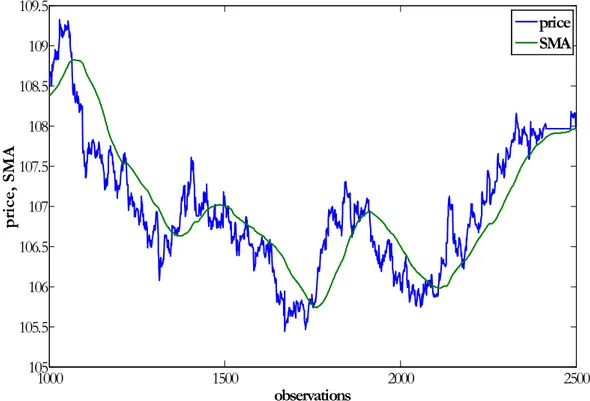
Dans la thèse on considère trois types des bandes qui correspondent aux groupes présentés plus haut. En première partie on estime la ligne centrale optimale sous la forme de la moyenne mobile krigée (KMA), la deuxième et la troisième parties utilisent respectivement la moyenne mobile simple (SMA) et moyenne mobile exponentielle (EMA) en tant que ligne centrale. La partie II a examiné les bandes définies par les caractéristiques statistiques des données (par exemple, variance). La partie III a analysé les stratégies de trading pour les bandes créées par le déplacement parallèle de la ligne centrale en haut et en bas. Le choix de différents types de la moyenne mobile (KMA et SMA) pour les deux premières parties est justifié par la nécessité d’éviter de mélanger des effets de l'amélioration des bandes de trading provoquées par les optimisations de ses composants. Quant au choix des bandes en partie III est expliqué par l'énorme popularité de ce type de bandes chez les traders.
Dans la partie I "Optimisation de l’indicateur de la moyenne mobile: méthode de krigeage" on propose d’utiliser le krigeage, une approche geostatistique, pour l’optimisation des poids des moyennes mobiles (MA). Cette méthode permet d'optimiser la structure des poids pour une longueur prédéfinie de la fenêtre sur lequelle la moyenne mobile est calculée. La méthode de krigeage permet d’obtenir l’estimateur optimal, qui incorpore les caractéristiques statistiques des données, telles que la covariance (autocovariance). Cela permet d'obtenir des estimateurs optimaux qui dépendent des caractéristiques statistiques des données plutôt que des valeurs des données historiques comme dans le cas des études de simulation. Contrairement aux méthodes classiques, qui sont utilisées en finance, cette méthode peux être appliquée à deux types de
données: échantillonées à distance régulière ou irrégulière. Cette approche propose de définir le meilleur estimateur de la moyenne comme une somme pondérée des observations dans un voisinage, qui coïncide avec la définition de la moyenne mobile. La méthode d’optimisation se base sur la minimisation de la variance d’estimation.
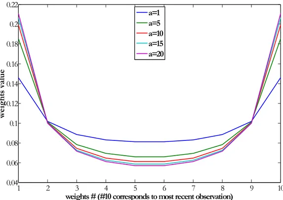
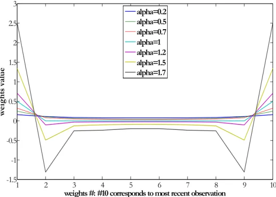
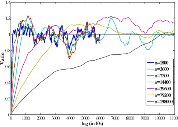
Nous avons vu que la meilleure moyenne mobile krigée (KMA), estimée sur les données régulières a une structure des poids spécifique pour certains modèles de covariance: les plus grand poids sont attachés à la première et la dernière observation, alors que tous les autres poids sont faibles. En conséquence, KMA oscille autour de la courbe de SMA. La volatilité et l'amplitude des oscillations est une fonction indirecte de la longueur du voisinage utilisé pour le KMA : le KMA sur un voisinage plus long est moins volatile et coïncide plus avec la courbe de SMA. Par conséquent, des stratégies de trend-following, qui sont basées sur les KMA et SMA prendront des positions différentes pour des voisinages courts et les même positions pour des voisinages grands. La structure des poids ne dépend pas de la longueur de la fenêtre mais du modèle de covariance. Ce dernier a un impact sur les valeurs des coefficients de pondération proches des bordures de la fenêtre : le moins régulier est le modèle de variogramme à l’origine le plus les poids de KMA sont proches des coefficients de pondération du SMA. Par example, le modèle effet de pépite amène aux poids optimaux qui correspondent aux poids de la moyenne mobile simple.
La structure des poids des échantillons à maille irrégulière est plus variable, elle dépend de l'écart entre les échantillons de la variable utilisée pour subordonner
les prix ou la distance entre les observations de prix temporaires: plus l'écart est grand, plus la structure des poids est volatile.
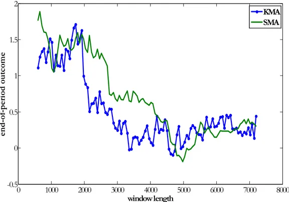
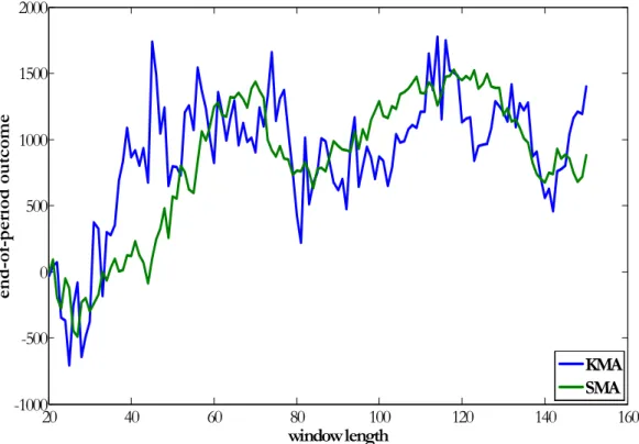
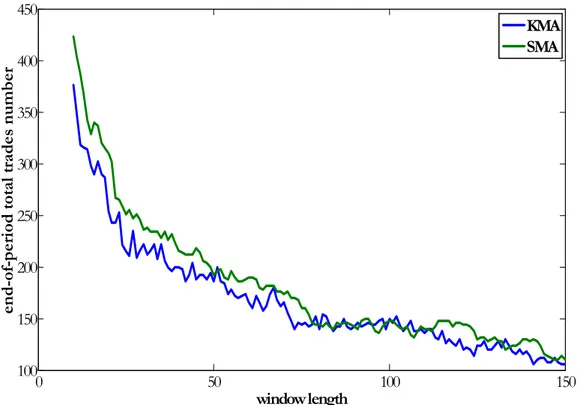
L’analyse du KMA en contexte de stratégies de trading montre que le KMA permet d’obtenir des résultats positifs et intéressants. Les résultats de l'application de stratégies « trend-following » définie par les croisements de moyenne mobile et de courbe des prix montrent que pour la majorité des instruments considérés KMA génère des résultats plus élevés que les moyennes mobiles simples ou exponentielles. En plus, le profit maximal etait obtenu pour des KMA sur de petits voisinages. Les moyennes mobiles traditionnelles sur des voisinages courts produisent normalement beaucoup de faux signaux et de ce fait sont moins rentables. Malgré son caractère volatile, KMA ne génère pas plus de transactions que les moyennes mobiles traditionnelles de même longueur. Par conséquent, il semble que la nature erratique de la courbe de KMA ne conduit pas nécessairement à générer plus de faux signaux pour les stratégies de trend-following.
L’application des stratégies de trading pour les échantillons irréguliers montre que les différents types de moyennes mobiles calculées sur l’échantillon ajusté (pour avoir un échantillon régulier) pourrait conduire à des résultats moins efficaces, que si on calcule la moyenne mobile optimale pour l’échantillon irrégulier par la méthode de krigeage.
La deuxième partie "Une alternative aux bandes de Bollinger: les bandes, basées sur les données transformées", propose une nouvelle approche pour optimiser les bandes de trading.
Bandes de Bollinger ont été proposése au début des années 1980 et restent très populaires parmi les professionnels de nos jours. Bollinger a proposé d'utiliser la moyenne mobile simple comme une ligne centrale:
n P m t n t i i t
∑
+ − = = 1avec
{ }
Pi 0≤i≤t,∀t >0 - la prix, - longeur de la fenetre. n Les bandes sont définies par l’ équation suivante :t t t m k b = ± σ , avec
(
)
n SMA P t n t i t i t∑
+ − = − = 1 2 2σ , ∀k =const >0- paramètres de Bollinger.
Les conclusions suivantes peuvent être dérivées pour les bandes de Bollinger : 1. Les bandes de Bollinger sont ajustées pour la volatilité des prix, comme
la définition des bandes incorpore l'écart-type, en tant que mesure de la volatilité.
2. Les bandes supérieures et inférieures au même moment de temps sont placés à distance égale de la moyenne mobile, c'est-à-dire ces bandes sont symétriques. Toutefois, cette distance peut être différente à différents moments du temps, en raison de l'évolution de la nature de la volatilité des prix.
3. La distance entre les bandes se réduit avec la diminution de la volatilité des prix et s’élargit avec l’augmentation de celle ci.
4. L'usage des SMA comme la ligne centrale est justifiée par le fait que le SMA est la moyenne statistique des prix des sous-échantillons - la même valeur qui est utilisée pour les calculs de l'écart-type de prix. En outre, certaines recherches montrent que la substitution de la SMA par
la moyenne mobile plus rapide ne produit pas de résultats plus élevés (Bollinger, 2002). Nous avons également montré dans la partie 1 qui moyenne mobile optimale krigée (KMA), en moyenne, coïncide avec la SMA : KMA coïncide avec le SMA pour les grandes longueurs de la fenêtre. L'intérêt de l'introduction de la moyenne mobile exponentielle (EMA) au lieu du SMA pourrait consister en méthode récurrente de son calcul (à l'heure actuelle EMA peut être calculée comme une somme pondérée du prix actuel et de la valeur précédente de l’ EMA). Toutefois, à cet égard SMA peut également être programmée avec des formules récurrentes, mais il a besoin d’accumuler plus de données à chaque instant que pour le calcul d'EMA.
La méthode traditionnelle de Bollinger est statistiquement justifiée pour les cas de prix au minimum localement stationnaires et avec une distribution symétrique. Les bandes, basées sur les données transformées, fournissent un moyen simple mais puissant pour l’optimisation des bandes. La méthode, est basée sur la transformation des données en une variable normale, qui permet de définir les valeurs extrêmes et en conséquence les valeurs des bandes sans imposition des contraintes sur la fonction de la distribution des résidus. Du point de vue théorique les bandes optimales devraient contenir K% des données (par exemple, K% = 90%); toutes les observations qui se trouvent en dehors des bandes sont considérés comme extrêmes. Les bandes ne sont pas faciles à définir pour la distribution asymétrique ou multimodale et exigent un temps considérable pour la procédure d’optimisation. Notre méthode permet d'obtenir les bandes dans un cadre plus simple et moins intensif en termes de calculs. Pour cette procédure, les données brutes (résidus) sont d’abord transformées en variables normales. Pour la variable normale la distribution est
connue et bien definie ; en conséquence les intervalles qui contiennent K% des données sont connus. Ensuite, les bandes pour les données brutes sont obtenues par transformation de l'intervalle (bandes) pour la distribution normale en utilisant d'une fonction d’anamorphose calibrée précédemment. Les DT bandes contiennent le même pourcentage de données que l’intervalle pour les données normales.
Nous avons examiné notamment les résidusRi =Pi −SMAt, =
∑
ii
t P
n
SMA 1 ,
pour calibrer la fonction de transformation. Notre objectif principal était de rester dans le contexte de la théorie des bandes de Bollinger qui utilisent ces résidus pour le calcul de l'écart-type des données. En même temps, ces résidus provoquent la forme specifique de ces DT bandes : les bandes forment un escalier qui change de marche si il ya une variation importante de prix. Cependant, les DT bandes sont moins sensibles à des mouvements non significatifs des moyennes mobiles. En plus, il semble que les DT bandes peuvent etre utilisées pour définir d’autres signaux de trading comme les vagues d’Elliot et niveaux Support/Resistance.
[
t n t i∈ − +1;]
On a analysé des stratégies différentes dans la partie II. Les stratégies de bande de Bollinger, comme toutes les stratégies contrariantes envoient de faux signaux au cours de la tendance présente dans les données à cause des erreurs qu'elles font dans la définition de la "vraie" valeur de l’instrument. Pendant les tendances des marchés la «vraie» valeur augmente ou diminue, par conséquent, des signaux de "surévaluation" ou "sous-évaluation" d’instrument sont fausses. Statistiquement, cela implique que les paramètres de nos bandes ne reflètent pas la vraie distribution de probabilité, qui n'est pas constante. En raison de ces
faux signaux les traders ne se basent pas uniquement sur les signes envoyés par les bandes de Bollinger, mais les examinent en combinaison avec d'autres signaux d’analyse technique, dans le but de confirmer la sur-évaluation / sous-évaluation ou de prédire les mouvements futurs des prix (par exemple, inversion de tendance). Dans cette partie nous avons examiné le momentum, comme l'un des signaux de confirmation pour les stratégies basées sur les bandes de Bollinger. Le même signal est utilisé pour la confirmation des stratégies pour les DT bandes. En outre, nous utilisons aussi les signaux de « Elliot » et « Support / Résistance » pour confirmer les signaux des DT bandes. À la suite, quatre stratégies différents sont analysées: (1) les stratégies de base, qui se fondent uniquement sur les signaux envoyés par les bandes, (2) les stratégies confirmées par le momentum, (3) les stratégies confirmées par les signaux d’ « Elliot » ; et (4) les stratégies confirmées par les signaux d’ « Elliot » et des « Support / Résistance ».
Les résultats de simulations trading pour quatre instruments différents montrent que les DT bandes génèrent plus de profits que les bandes classiques de Bollinger en stratégie confirmée par l’indicateur de momentum; les trajectoires de profil profits/pertes ont une pente plus positive et ascendante. Les majorités des stratégies gagnantes incorporent les DT bandes. En particulier, les stratégies marchent bien pour trois des quatre instruments. En plus, la stratégie de DT bandes était encore rentable en présence des certains coûts de transaction et de slippage. Enfin, les DT bandes pourraient être utiles dans la définition d'autres règles d’analyse techniques - les vagues d'Elliot et les niveaux de support / résistance. En conséquence, les nouvelles DT bandes ne sont pas seulement mieux justifiée d'un point de vue statistique et plus simples
dans leur application, mais elles permettent également générer des profits plus importants.
La partie III "Le krigeage disjonctif en finance: une nouvelle approche pour la construction et l'évaluation des stratégies de trading» présente l’application des méthodes de krigeage disjonctif (DK), pour des décisions plus informative en termes de timing et type de position. Comme beaucoup des stratégies de trading sont basées sur des signaux envoyés par la rupture de certains seuils, ces problème demande plus d’attention. Le krigeage disjonctif, une autre approche géostatistique, permet d’estimer les probabilités, que certain seuils seront atteints dans le futur.
En particulier, nous voulons prédire la probabilité conditionnelle
(
Zt zc Zt Zt Zt mP +Δ < , −1,..., −
)
sur la base des dernières observations disponibles dans certains voisinages. Du point de vue statistique, nous avons besoin de connaître la distribution Z( )
T Zα à (n+1)-dimensions, qui est compliquée, voire impossible à estimer à partir de données empiriques. La méthode de krigeage disjonctif implique seulement la connaissance de la distribution bidimensionnelle{
Z( )
ti ,Z( )
tj}
,0≤i< j≤n et( )
( )
{
Z T ,Z tj}
,0≤i< j≤n comme une condition nécessaire pour les calculs dela prédiction d’une fonction non linéaire. Il s'agit d'une hypothèse moins stricte que la connaissance de la distribution à (n+1)-dimensions.
La méthode de krigeage disjonctif est basée sur l'hypothèse qu’une fonction non linéaire de certaines variables aléatoires peut être développée en termes de facteurs d’un polynôme:
( )
[ ]
[ ]
( )
[ ]
( )
∑
∞[ ]
( )
= = + + + = 0 2 2 1 1 0 ... k k kH Y t f t Y H f t Y H f f t Y fQuand Y
( )
t est une variable normale et les couples{
Z( )
ti ,Z( )
tj}
,0≤i< j ≤nont une distribution bivariable gaussienne, nous pouvons utiliser des polynômes orthogonaux d’Hermite pour le développement de la function non-linéaire. Grace à l'orthogonalité des polynômes de Hermite, le krigeage disjonctif de la fonction non linéaire est réduit au krigeage des polynômes de Hermite.
Pourtant l'application de la méthode de krigeage disjoncitif à données financières demande quelques ajustements en raison de la particularité de celles ci. Un des problèmes est la non-normalité de la variable analysée. En ce cas la variable et les seuils sont transformés en variables normales. Le principal problème est pourtant la non-stationnarité qui exige la ré-estimation des paramètres de la méthode, notamment de la fonction d’anamorphose. Nous avons proposé la méthode qui permet d’ajuster la fonction de transformation principale (basique) à la volatilité locale des données.
Deux types de probabilités disjonctives peuvent être définis et évalués. Les probabilités disjonctives ponctuelles sont les probabilités estimées par krigeage disjonctif en des points particulier ; ils reflètent la probabilité qu’un certain seuil sera dépassé à un certain moment de temps. Cette probabilité peut être estimée, mais ne peut pas être validée. Le krigeage disjonctif d’un intervalle reflète la probabilité qu’un certain seuil sera dépassé sur un intervalle de temps futur. Ce type de probabilité peut être validé par les fréquences empiriques - la proportion des observations lorsque le prix a été au-dessous d’un certain seuil.
Ces probabilités ont été estimées pour quatre instruments différents. Les résultats sont cohérents. L'intervalle DK probabilité (calculé pour la fonction d’anamorphose constamment ajustée à la volatilité locale) démontre une bonne prédiction en termes de timing et des valeurs en comparaison avec les fréquences empiriques. Nous avons également montré que seule la longueur de l'intervalle pour lequel la prévision a été faite et la longueur de l'échantillon utilisé pour l'ajustement de la fonction d’anamorphose ont un impact sur la prévision par la méthode de krigeage disjonctif.
La pouvoir de la prédiction de la méthode de krigeage disjonctif a été évalué aussi par la comparaison des résultats des stratégies de trading, qui incorporent cette probabilité krigée. Nous avons construit deux types des stratégies: (1) stratégie de krigeage disjonctif, où la décision sur la position d’entrée est faite sur la base des probabilités krigées, et (2) la stratégie aléatoire, où la décision sur la position d’entrée est faite au hasard (avec probabilité de 0.5). Notre étude révèle que la stratégie de krigeage disjonctif produits des résultats positifs pour l'intervalle continu des seuils. La stratégie aléatoire produit les bénéfices à nature aléatoire. La distribution de profit per transaction montre que le krigeage disjonctif permet de diminuer le nombre de transactions avec les pertes et augmenter la nombre de transaction avec les profits, si on compare avec la distribution de la stratégie aléatoire, qui produit une distribution symétrique pour les gains des transactions.
En conséquence, nous avons montré comment cette méthode peut être appliquée / ajustée pour les données financières d’une manière continue que
par rapport à la stratégie aléatoire, la stratégie de krigeage disjonctif améliore le processus de prise de décision.
Dans ce travail, nous sommes concentrés sur des études d’application d’analyse technique et ses stratégies à un seul instrument. Les recherches futures devraient envisager l’optimisation des stratégies pour un portefeuille d'instruments. En particulier, une autre méthode géostatistique multivariable, telle que cokrigeage peut être utilisée pour l'estimation de la moyenne du portefeuille et la prévision de sa valeur.
Afin de séparer les effets de l'amélioration de la ligne centrale (par l'introduction de la KMA) et l'amélioration de bandes (par l'introduction de la DT bandes), nous n'avons pas examiné les DT bandes qui intègrent la KMA comme la ligne centrale. Il serait particulièrement intéressant d’analyser des stratégies, fondées sur les DT bandes et KMA court.
L’approche des DT bandes indique les directions suivantes de recherche seraient à envisager. L'ajustement de la fonction d’anamorphose à la volatilité locale, réalisée dans la partie III pour la méthode de krigeage disjonctif, peut être appliquée à la définition des DT bandes.
L'étude de la relation entre la rentabilité de la stratégie et la valeur de paramètre
K% utilisée pour la définition des DT bandes permettra augmenter les profits
des stratégies définies sur la base de ces bandes.
Cette approche crée des nouvelles possibilités à l'amélioration d'autres instruments et règles d'analyse technique. Par exemple, la stratégie confirmée
par l’indicateur de momentum est fondée sur la définition des seuils optimaux pour cet indicateur. Dans cette analyse les seuils n’étaient pas optimisés, mais l’approche de transformation des donnée utilisée pour la définition des DT bandes peux être utilisée pour définir les seuil de momentum. Cela pourrait conduire à des seuils asymétriques de momentum. L'autre exemple est l'application des DT bandes à la définition d'autres indicateurs techniques, comme les vagues d'Elliot et de support / résistance.
Enfin, l'application de la méthode de krigeage disjonctif aux données financières peut encore être améliorée par un meilleur ajustement de la fonction cumulée de la distribution utilisée pour la transformation de données aux changements de moyenne locale ou à l’asymétrie de distribution.
Les résultats d’analyse prouvent que les techniques proposées dans cette thèse sont prometteuses et peuvent être utilisées en pratique. Ils indiquent aussi de nombreux domaines de recherche pour l'avenir.
Contents
General Introduction ………. Part I : Moving average optimization: kriging approach ………...
Introduction ……….. 1. Moving average as a trading instrument………... 1.1. Definition of moving average ………...………. 1.2. Types of the moving average ………. 2. Kriging method: Theory ………. 2.1. Geostatistic instruments and terminology: short overview …….……….
2.1.1. Stationary and intrinsic stationary functions ……….…..
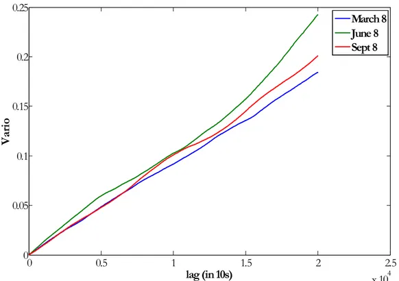
2.1.2. Variogram ………..
2.2. Simple kriging: prediction of the process with zero mean ………... 2.3. Simple kriging: prediction of the process with known mean ……….….. 2.4. Ordinary kriging: prediction of the process with unknown mean ……….….. 2.5. Ordinary kriging: estimation of the unknown mean ………... 2.6. Kriging non-stationary variable ……….. 2.6.1. Universal kriging: trend estimation ………. 2.6.2. Kriging intrinsic function IRF-0 ………. 3. Peculiarities of the kriging method applications in finance ………
3.1. Data non-stationarity ………. 3.2. Data sampling peculiarities ……… 4. Kriging results: non-stationary, evenly spaced time-series data ………. 4.1. Variogram analysis and optimal kriging weights: Bund ……….. 4.2. Trading results: kriged moving average versus simple moving average …………..
4.2.1. Bund ………..
4.2.2. DAX ………..
4.2.3. Brent ………..…
4.2.4. X instrument ………..
5. Kriging results: bounded, evenly spaced time-series data ………... 5.1. MACD and trading strategies ………. 5.2. MACD strategy: optimal signal line ………... 5.3. Results of the trading strategy, based on the MACD indicator and signal line ……
5.3.1. Bund ………..
5.3.2. DAX ……….
5.3.3. Brent ……….
5.3.4. X instrument ……….
6. Kriging results: unevenly spaced data ………... 6.1. Unevenly spaced time dependent price series ………... 6.2. Unevenly spaced price series subordinated to cumulative volume ……….. 7. Conclusions ………. 8. Appendices I ………... Part II. An Alternative to Bollinger bands: Data transformed bands ………
Introduction ………... 1. Classical Bollinger bands concepts ………...….. 1.1. Bollinger bands definition ……… 1.2. Bollinger bands and trading strategies ……….. 1.3. Theoretical framework for Bollinger bands ……..………..……….. 2. Data transformed bands ………..………... 2.1. Data transformed bands: algorithm description ……….. 2.2. Data transformed bands: empirical observations ……….…. 2.3. Data transformation bands: other technical rules description ………... 3. Strategies descriptions ……… 1 12 12 14 14 14 16 17 18 19 21 23 24 25 26 27 28 30 31 31 33 38 38 46 47 49 51 53 55 55 57 59 61 63 65 67 68 70 75 83 86 111 111 114 115 117 121 124 125 127 128
3.1. Strategies ……… 3.2. Choice of the streategy parameters ………. 3.3. Analysis of the outcomes ……… 4. Trading outcomes for different instruments ………...…………
4.1. Bund …...……… 4.2. DAX ………... 4.3. Brent ………... 4.4. Instrument X ……...……… 5. Conclusions ………...………..… 6. Appendices ………...………..………... Part III. Disjunctive kriging in finance: a new approach to construction and evaluation of trading strategies
Introduction …...………. 1. Theory ………...……….
1.1. Disjunctive kriging ………...………… 1.2. Disjunctive kriging: normal random process ……….... 1.3. Disjunctive kriging: non-normal random process ……… 1.4. Disjunctive kriging: case of regularized variable ………... 1.5. Disjunctive kriging: particular case of the variable with exponential covariance
model ……….. 2. Peculiarities of the disjunctive kriging application to the financial data ……….. 2.1. Calibration of the transform function: kernel approach ………... 2.2. Data used for the estimation of the CDF: locally adjusted transform function …. 3. Examples of the DK probabilities under stationarity assumption………
3.1. Point DK probabilities: DAX case ...……… 3.2. Interval DK probabilities for global transformation function: Bund case ………. 4. Examples of the DK probabilities under local stationarity assumption ………..
4.1. Framework for the estimation and analysis of the interval DK probabilities …… 4.2. Interval DK probabilities: DAX instrument ………. 4.2.1. Impact of the window length ………
4.2.2. Impact of the interval length ..……… 4.2.3. Impact of the DCI length ….………. 4.2.4. Impact of the bandwidth parameter ……… 5. Application of the DK method to the strategy construction ………
5.1. DK trading strategy ……… 5.2. Random walk (or benchmark) strategy ……….
5.3. Strategies outcomes .……….. 5.3.1. DAX ………. 5.3.2. Bund ...………. 5.3.3. Brent ………. 5.3.4. X instrument ………. 6. Conclusions ………. 7. Appendices III ……… General Conclusions ………. Bibliography ……….. 132 132 136 138 139 139 145 152 157 161 164 180 180 182 183 185 189 189 190 192 193 199 202 202 205 212 212 215 216 218 220 222 223 224 224 225 226 228 231 233 235 238 252 255
General introduction
Technical analysis is a hotly debated topic among researchers and traders. It has its devoted supporters, so called technicians or technical analysts, as well as the opponents who do not accept its methods. The debate takes place not only between different groups of traders (fundamentalists vs. technicians1), but also between the representatives of academic circles and
traders (technicians). The discussion between different types of traders is explained by different principles and relationships that are used for predicting future prices. Fundamentalists base their predictions and, thus, their strategies on the market fundamentals, such as macro-indicators and micro-indicators. Macro-indicators evaluate general market situation; inflation, interest rate, unemployment rate, inventories, consumer confidence index, etc. are the examples of such indicators. Micro-indicators represent the characteristics of an instrument, for which the prediction is made; for example, for the prediction of the price movements of a particular stock, the traders analyze company’s revenues, assets, balance sheet, etc.
In their turn, technical analysts believe that prices incorporate all information available in the market (i.e. macro-, micro-indicators, expectations, etc.). Therefore, arguably, it is sufficient to use the existing price observations to make predictions about future price movements. Thus, technical analysis techniques are predominantly based on the price data.
When it comes to the academic audiences, most of them2 refuse to accept technical analysis as a
consistent price forecast method. As noted Lo et al. (2000), many academic researchers who easily accept fundamental factors believe that “the difference between fundamental analysis and technical analysis is not unlike the difference between astronomy and astrology”3. Taking into
account that the technical analysis exists for more than 100 years, such resistance of the researchers is quite puzzling, and we believe that there may be an explanation to this phenomenon.
First, the technical analysis theory is based on the assumption that the past price observations can be used to predict the future price movements. This assumption contradicts the efficient market hypothesis (EMH)4 that is the cornerstone of the financial theory and on which many financial
models are based. At the same time many departures from EMH are observed in the real markets due to over- or under-reaction, certain market anomalies (such as size effect), behavioral effects. Bernard and Thomas (1990), Banz (1981), Roll (1983), Chan, Jegadeesh, Lakonishok (1996), Huberman and Regev (2001) are the examples of such research. Treynor, Ferguson (1984) demonstrated theoretically that past prices, combined with other information, can predict the future price movements. Lo and MacKinaly (1988, 1999), showed that past prices can be used as a forecast for future prices. Finally, Grosman and Stiglitz (1980) argue that mere presence of the trading and investment activity and the possibility to earn profits in financial markets undermines the credibility of EMH. Despite the existence of such anomalies, the supporters of EMH still believe that the investment opportunities occur only in the short-term, and they are eliminated in
1 Nowadays pure technicians or fundamentalist among traders rarely exist. Technicians generally do follow the
financial news and the macro-indicators, while fundamentalists apply some of the technical analysis techniques.
2 Some researchers though believe in the prediction power of the technical analysis. Further we will provide these
works in general literature review.
3 Lo, A. W., Mamaysky, H. and J.Wang. 2000. “Foundations of Technical Analysis: Computational Algorithms,
Statistical Inference, and Empirical Implementation”, The Journal of Finance, Vol. LV, #4 (August, 2000), pp.1705-1765, p.1705.
4 The EMH states that the more efficient the markets are, the more random the price movements in these markets
are. As a result, it is impossible to use the past prices to predict the future movements under this hypothesis. Literature review on the EMH can be found in Lo (2007).
the long run. As a result, at present there is no consensus regarding the validity of the EMH in real markets.
The second point is that most technical analysis techniques have been developed on the basis of the empirical observations, rather than derived or modeled mathematically. For example, the majority of chart patterns, such as “Support/Resistance”, “Head-and-Shoulders”, etc. were the results of regular observations of the price behavior. Evidently, the experiment and observation laid the foundation for many major inventions in physics, mechanics, chemistry and engineering. The key difference between the scientists and technicians appears to manifest itself in the way they treat the observed results: contrary to the scientists, technicians frequently do not bother to prove or explain their observations, but take them for granted.
The third explanation is driven by the fact that the technical trading rules are often unjustifiably presented as “optimal”. We can frequently see the traders making claims about “optimal” values of certain technical parameters (for example, the moving average length) without any additional support or explanations how and for what data type (instrument, data frequency, etc.) these values were obtained. Obviously, such statements raise lots of skepticism from the scientists. Finally, the “language barriers” created by the usage of the technical jargon on one side and statistical terms and tests names on the other complicate the assimilation of the new ideas by both sides (Lo et al., 2000). In addition, the researchers frequently mistakenly believe that the technical instruments are only about “charting”, disregarding the mathematical concepts that are used in building the technical strategies (for example, moving average, momentum, etc.)
Thus, we can conclude that the absence of both the scientific representation of the method and of a formal analysis of the method’s prediction power creates a misunderstanding between the technical traders and academic researchers. As defined by Neftci (1991), “technical analysis is a broad class of prediction rules with unknown statistical properties, developed by practitioners without reference to any formalism”5.
On our part, we believe that technical analysis should be viewed more as a “bank” of empirical observations of the financial markets that can be further used by the researchers to develop models or well-defined statistical trading techniques. We also believe that all the academic research performed to-date in this field, is a necessary input in narrowing the gap between the theoretical and practical finance.
According to some researchers, technical analysis studies can be split into the following groups: • Trend studies
This group represents the indicators that identify the trend and the trend breaks. Among the most popular indicators are moving averages, support and resistance levels, etc.
• Directional studies
This group contains the indicators that define the length and strength of current trend/forecast. Among these indicators are DMI, Parabolics, range oscillator, etc. • Momentum studies
This group concentrates on the measurements of the velocity of the price movements. The examples of such indicators are Stochastic, Momentum, Rate of
5 Neftci, S. N. “Naïve Trading Rules in Financial Markets and Wiener-Kolmogorov Predicition Theory: A study of
change, MACD, Trix and CCI. Momentum instruments are frequently used for the definition of the trend breaks that often follow the slowness of the price velocity. • Volatility studies
This group presents the trading rules that incorporate instruments’ volatility and the notion of extreme values. The examples of such rules are trading bands, among which the most popular case is the Bollinger bands.
• Volume studies
In the context of the technical analysis, volume is the second (after price) important data element that measures the trading activity in the markets. Volume itself as well as the indicators that incorporate volume information (for example, volume weighted moving averages) completes this group.
Each group of technical studies contains indicators and chart patterns. Indicators cover all buy/sell rules that are formulated on the basis of the well-defined mathematical expressions (for example, trading rules based on the moving average). In contrast, the charts cannot be explicitly defined by formulas; they are the graphical patterns defined subjectively by a trader. Therefore, one trader can recognize a specific chart as particular price pattern, while the other trader would see no pattern at all. The examples of such charts are Support/Resistance levels, Head and Shoulders and Triangles. It should be noted that researchers try to program the chart patterns by algorithms and estimation methods (see Lo et al., 2000), however, the results of the chart pattern recognition depends on the algorithm itself.
The financial literature that exists in the field, can be split into the following groups:
1. Development of the scientific framework and formalization of the technical analysis. 2. Evaluation of the prediction power of technical trading rules, as well as their comparison
with other prediction methods.
3. Analysis of the statistical properties of technical indicators and their trading outcomes. 4. Optimization of the existing indicators/rules/strategies; their improving; development of
the new technical trading instruments.
For the first group of studies6, the cornerstone work is the paper by Neftci (1991) “Naïve
Trading Rules in Financial Markets and Wiener-Kolmogorov Prediction Theory: A study of Technical Analysis”. It proposes the general approach that defines which technical rules can be formalized and which cannot. According to this framework, a well-defined rule should be a Markov time, i.e. it should use only information available up to current moment for its construction7. Most of the prediction technique that is used for financial market forecasts lies in
the Wiener-Kolmogorov prediction theory framework, according to which “time-varying vector autoregressions (VARs) should yield the best forecasts of a stochastic process in the least square error (MSE) sense”8. However, this framework is not suitable for the forecast of the non-linear
series. For example, Neftci (1991) defines at least two cases when linear models cannot produce plausible forecasts such as (1) producing sporadic buy and sell signals (non-linear problem by its nature); and (2) predicting some particular patterns, such as stock exchange crashes. Consequently, any other systems of forecasts that can predict non-linear time series can improve the forecast proposed by the Wiener-Kolmogorov framework. Similar conclusions are obtained in Brock, Lakonishok and Lebaron (1992). According to Neftci (1991), it may be the case that technical analysis informally tries to analyze the information captured by the higher order moments of asset prices. In fact the patterns and rules of the technical analysis can be
6 See also Rode, Friedman, Parikh, Kane (1995) for formalization of the technical analysis. 7 The method will be presented further in more details.
8 Neftci, S. N. “Naïve Trading Rules in Financial Markets and Wiener-Kolmogorov Predicition Theory: A study of
characterized “by appropriate sequences of local minima and/or maxima”9, that lead to
non-linear prediction problems (Neftci, 1991). As the result, he believes that technical analysis can improve the forecasts of the future price movements.
Another part of the formal academic research that can diminish the number of skeptics about the technical analysis is the formalization of the technical indicators and instruments themselves. While there is a lot of literature devoted to the description, definition or calculations of the technical indicators (Murphy, 1999; Achelis, 2000), there are few works that explain or justify the method from theoretical standpoint; the examples are Bollinger (2002) on the Bollinger bands, Ehlers ([38]) on moving average. Group of papers try to explain the predictability of the technical indicators in the context of the microstructure theory through the relationship between technical analysis and liquidity provision. The researchers believe that the technical analysis may indirectly provide information captured in limit-order books to make predictions about future price movements. Osler (2003) provided the explanation of the prediction power of such technical trading rules as Support/Resistance, proving the following hypothesis: the clusters of take-profit and stop-loss orders are the reasons why the rules succeed in predicting future price movements. Kavajecz, Odders-White (2004) related the moving average indicators (price moving averages of different length) to the relative position of depth on the limit order book.
The second group of studies that measure the predictive properties of the technical analysis is best represented in the financial literature. The majority of the papers in this field are devoted to the statistical (econometric) analysis of the prediction power of the technical rules, while comparing them with other (non-technical) predictors or variables. The early works in the field of the technical analysis did not find the superior prediction properties of the technical rules comparing them with the Buy-and-Hold strategy; as the result these works supported the EMH theory (Alexander, 1961, 1964; Fama and Blume, 1966; James, 1968; Van Horne and Parker, 1967; Jensen, Benington, 1970). More recent work by Allen, Karjalainen (1999) and Ratner and Leal (1999) has also found little evidence in favor of the technical analysis. At the same time other research provides the evidence in favor of the technical analysis. Brock, Lakonishok and Lebaron (1992) showed that 26 technical trading rules applied to Dow Jones Industrial Average over 90 years over-perform the strategy of holding cash. Sullivan, Timmermann, White (1999) shows that some of the technical rules considered in Brock et al. (1992) are actually profitable even after using the bootstrap method to adjust for the data-snooping biases. Levich, Thomas (1993) found that some moving average and filter rules were profitable in the foreign exchange markets. Osler, Chang (1995) also found the evidence of the profitability of the “head-and-shoulders” patterns in foreign exchange markets. Lo, Mamaysky, Wang (2000) showed that the same technical charts provide incremental information about future price movements by comparing unconditional distribution of the stocks returns with the conditional distribution of the returns (conditional on the presence of the chart pattern). Blume, Easley, O’Hara (1994) demonstrated that the traders who use information contained in the market statistics such as prices and volume do better than the one who do not use it. In this context, technical analysis is a component of trader’s learning process. Blanchet-Scallient et al. (2005) compare the results of the technical rules to the strategies, based on the mathematical model. Under certain assumptions (prices follow one-dimensional Brownian motion, trader’s wealth utility is represented by the logarithmic function) they show that MA rule can outperform the strategies based on the mathematical models in case of severe misspecifications of the model parameters.
As for the third group of studies, Acar, Satchell (1997) analyzed the statistical properties of the returns from the trading rules, based on the moving averages of the length 2. They showed that
9 Neftci, S. N. “Naïve Trading Rules in Financial Markets and Wiener-Kolmogorov Predicition Theory: A study of
in the case when the asset price distribution is a Markovian process, the characteristic function (and, therefore, the distribution function too) of the realized returns could be deduced.
The optimization of the technical trading rules has a crucial importance for the traders, who use this approach in the construction of their strategies. Both researchers and traders contribute to this field of studies. For some instruments that are more popular, many optimization approaches exist, while for the other the niche is largely underdeveloped. For example, many works devoted to the optimization of the rules based on the moving averages, momentum (Gray, Thomson, 1997). Certainly, the choice of the optimization techniques largely depends on the type of the technical indicator. However, there is one approach that is applied to many different techniques – a simulation of the trading strategy based on the available historic data samples. According to this approach the optimal parameters correspond to the global/local maximum or minimum of the trading outcomes (profit/losses, Sharpe ratio, number of trades, etc.). The example of such optimization approach can be found in Williams (2006). Although this approach is universal, as it can be applied to all rules that are used in the trading strategies, the method has its drawbacks. The outcomes are dependent on the historical data used for optimization; thus, the parameters optimal for the studied data set might be no longer optimal for a new data sample.
Finally, the development of the new instruments is a very dynamic field that is constantly enlarging both with the new types of the existing instruments and totally new ones. For example, Arm ([11], V.8:3) proposed the volume-weighted moving average, Chande ([28], V.10:3) developed the volatility adjusted moving average, Chaikin and Brogan in their time introduced Bomar bands (Bollinger, 2002).
As we can see, the majority of the papers in the field of technical analysis are devoted to the analysis of its prediction power within the context of EMH. Despite a significant number of papers on this topic, there is still no consensus whether technical analysis has superior prediction power over other prediction methods. Therefore, we will accept the hypothesis, similar to one in Grosman and Stiglitz (1980), that survival of the technical analysis among traders for the past 100 years can be considered a proof that it can be integrated into profitable trading strategies, at least for some particular instruments; otherwise the traders would have stopped using it.
At the same time, fewer researchers concentrate on the development of the theoretical framework for the analysis and optimization of the technical rules, although there is a pool of users (traders, technicians) who create the demand for this type of research. Thus, in this thesis, we want to concentrate on the optimization and development of the new trading techniques based on the existing technical strategies. The technical indicators/rules chosen for the analysis will be formalized and explained from the point of view of the statistical theory. Contrary to many existing works in the field that use trading simulations to define the optimal parameters, we want to use the optimization approaches, based on the statistical characteristics of the data in the first place. We will use the trading simulations in all parts of this thesis, mainly to compare the optimized indicator/strategy with other non-optimal (in the context of this work) indicators/strategies.
It is obvious that an exhaustive analysis of all technical rules is quasi-impossible: the set of trading rules is extremely large and it expands constantly with the development of the new rules and patterns. We decided to concentrate our analysis on such popular technical analysis techniques as trading bands. While being part of the volatility studies, trading bands frequently incorporate (in their constructions or their strategies) other techniques of the technical analysis from such group of studies as trend and momentum (see classification above). Besides, we will prove that the
method itself is well defined within the framework developed by Neftci (1991), briefly presented further.
Trading bands are lines plotted around a measure of central tendency, shifted by some percentage up and down (upper and lower bands) (Bollinger, 2002). The schematic representation of the concept is given in Figure 1.
Trading bands have four key components (see Figure 1): (1) price (quotes),
(2) mid-line, (3) upper band, and (4) lower band.
The way these components are defined implies the existence of different bands types, such as envelopes and channels (Bollinger, 2002, Murphy, 1999).
Upper band
Lower band
Central tendency
Figure 1. Schematic representation of trading bands
Despite the differences in constructing the bands, the strategies based on them are quite similar. Touching/breaching upper/lower bands give trader information on the direction of price movements or on relative price levels (whether the instrument is oversold or overbought), which are used as signals in strategy construction. As a result, both trend following and contrarian strategies can be defined on the basis of the trading bands.
For example, let some moving average represent the mid-line in the bands. Suppose prices crossed the upper band of the trading bands after continuous fluctuations within the upper/lower bands and the mid-line crossing. For the trend following strategy, the bands are the confirmation of an established trend: the first signal that the upward trend had been established happen at the crossover of the moving average and price curve10. Therefore, a breach of the
10 Breaching the upper bands implies that the price has been previously breaching the moving average line from
upper band can be used as a confirmation signal of an upward trend. In this context, trading bands allow to eliminate false signals generated by the moving average trading rule.
Breaching the trading bands in the context of the contrarian strategy confirms that the instrument is mis-priced. Therefore, breaching the upper band means that currently the instrument is overpriced and the price should return to its average (moving average line) in future.
As the same trading bands can be used in the strategies that lead to the opposite trading decisions11, traders frequently use trading bands in combination with other technical trading
signals that confirm the presence or absence of a trend. In case of the trend-following strategy, these extra rules give additional confirmation signals that the trend has been established, while in the case of the contrarian strategies they allow avoiding trending patterns, where contrarian strategy sends false signals.
As have been mentioned already, it can be proven that some types of the trading bands are well defined. According to Neftci (1991), technical trading rule is well defined if it is a Markov time. Let be an asset price; - sequences of information sets (sigma-algebras) generated by and other data sets observed up to time t.
{
Xt}
It XtDefinition 1
A random variable τ is a Markov time if the event At =
{
τ <t}
is –measurable. ItSimply speaking, it means that a rule/indicator is well defined if for making a decision or its calculation it uses only information available up to the current moment, but not the one that anticipates the future. For example, the first moment of time when prices increase 20% from the initial level at is Markov time: on the basis of available history of prices up to moment , we can determine whether this event has happened or not. As a result, the Markov time approach eliminates many technical rules that anticipate the future, among which many chart patterns.
0 =
t t
The definition of a technical rule as a Markov time implies (1) possibility to quantify the rule, (2) feasibility of the rule, (3) possibility to investigate rule’s predictive power. However, the fact that the rule is well defined cannot justify its usage. In order to be used, a rule should produce (buy/sell) signal at least once, i.e. the probability that the signal is generated at least once should be equal to one (see Definition 2).
Definition 2
A Markov time τ is finite if
(
τ <∞)
=1P .
In addition, a rule should have at least the same predictive power as other well-defined forecasting techniques. As a result, a trading rule gives a consistent forecast of the future price movements if it is a finite Markov time that has at least the same predictive power as more formalized forecasting methods. For example, Neftci (1991) showed that the moving average trading rules are finite Markov times and in some cases have higher predictive power than the linear forecast methods, such as AR or ARMA models.
11 The trading positions taken within each strategy would be the opposite: for the trend-following strategy a long
Further we provide the proof that the trading bands are Markov times.
Lets define
{
as some random process that represents price time series; as a sequences of information sets (sigma-algebras) generated by and other data sets observed up to time t. Trading band is defined as following:}
t X It t X • middle line: ; mt • upper bands: (1), ; t t m +δ δt(1) >0 • lower bands: (2), . t t m +δ δt(2) <0Proposition 1
Let functions mt, , be -measurable. Lets define the following variables:
) 1 ( t δ (2) t δ It t t t X m Z = − (1) ) 1 ( ) 1 ( t t t Z Y = −δ (2) t t t Z Y(2) =δ(2) − (3) Then,
• generated times { }entry i τ :
[
: 0]
inf (1) (2) 1 ⋅ ≤ > = − t t entry i t entry i t τ Y Y τ , τ0entry =0, (4) are Markov times.• generated times { }exit i τ :
[
: 0]
inf > ⋅ 1 ≤ = entry t t− i t exit i t τ Z Z τ , (5)are Markov times.
Proof.
Note that , , are -measurable. This implies that the products and are also -measurable. and are defined as the first entry of and in the interval
(
respectively. Then, according to the Theorem (Shiryayev, 1985), which states that the first entry of the processt Z Yt(1) Yt(2) It Zt ⋅Zt−1 ) 2 ( ) 1 ( t t Y Y ⋅ It entry i τ exit i τ (1) (2) t t Y Y ⋅ 1 − ⋅ t t Z Z − 0∞;
]
∈ℜ{ }
Xt in some defined interval is alwaysMarkov time, the entry and are Markov times.
i
τ exit
i
τ
Proposition 1 states that if estimates of the middle line and trading bands are defined on the basis of the information available up to moment t , the trading rules based on these trading bands is well-defined. For example, moving average that is often used as the middle line is -measurable. Constant scalars , together with the -measurable middle line define bands, which are -measurable. Finally, Bollinger bands, with the middle line
∑
= − + = n i i n t i t w X MA 1 t I δt(1) ) 2 ( t δ It t I∑
= − + = n i i n t t X n MA 1 1 and δt = δt =kσt ) 2 ( ) 1( , where >0some scalar,
k σt - experimental standard deviation of the
{ }
Xi t− 1n+≤i≤t, are also -measurable. ItNote that the trading strategy defined in Proposition 1 is as follows: a position is opened when the price breaches one of the bands; this position is closed, when the price crosses the middle line.
Proposition 1 demonstrates that there are trading bands strategies that can be considered as well defined. The question is now whether the signals they send are finite, i.e.
(
entry <∞)
=1Pτ ,
(
exit <∞)
=1Pτ . It is obvious that the distance between the bands defines whether these trading
bands will send finite signals. In particular, if the distance between the two bands is extremely large the entry signal might never be generated. The entry signals will be generated for the stationary process
{
Xt}
and unbiased estimator of its mean mt, if the following inequality holds:(
)
1 0< + (2) < < + (1) < t t t t t X m m P δ δ (6)The expression (6) can be considered as criteria for the choice of the distance ( )1 ( )2
t t δ
δ +
between the bands that can generate any entry signals. As for the exit signals, Neftci (1991) showed that the trading rules, based on the cross-over of price and MA curves, generate finite signals in the case when price process
{ }
Xt is stationary and m-dependent price process.The majority of the trading bands used by traders incorporate moving average as middle line. Moving average allows constructing well-defined trading bands; therefore, we will narrow our analysis to this particular type of bands. Such trading bands are the function of four different parameters or vectors of parameters:
{ }
(
n wi i n dU dL)
f
TB= , 1≤≤ , , ,
where - parameters of the moving average: length of the moving window and weights attached to the price in the window (see Ch.1.1 for more details);
{ }
wi i nn, 1≤≤
L U d
d , - distance between moving average and upper and lower bands respectively. Note that
upper and lower distances can be different, as well as each distance itself can be a function of time: dU ≠dL, d( ) =d
( )
t .Despite the large number of the bands parameters, their optimization can be simplified:
1. Search for the optimal parameters for middle line and bands can be separated due to the different roles that they play in the definition of the trading bands strategy. For example, within the context of the contrarian strategy moving average represents the mean value of the instrument, while bands define the extreme values of the prices conditionally on the current mean. We do not need to know the bands value in order to evaluate price mean, while we need a current mean value (and probability distribution function) to define the extreme values, and thus, bands. As a result, the band optimization problem can be split: first, best middle line estimator (its parameters) is obtained, then optimal bands parameters are searched for.
2. According to Proposition 3, the optimal moving average should be the best estimator to the local mean (or trend). This allows choosing clearer and more objective optimization criteria - minimization of the mean squared error:
(
Mˆt −mt)
2 →minE ,