HAL Id: hal-01183149
https://hal.archives-ouvertes.fr/hal-01183149
Submitted on 6 Aug 2015
HAL is a multi-disciplinary open access archive for the deposit and dissemination of sci-entific research documents, whether they are pub-lished or not. The documents may come from
L’archive ouverte pluridisciplinaire HAL, est destinée au dépôt et à la diffusion de documents scientifiques de niveau recherche, publiés ou non, émanant des établissements d’enseignement et de
Uncertainties in structural dynamics: overview and
comparative analysis of methods
Sami Daouk, François Louf, Olivier Dorival, Laurent Champaney, Sylvie
Audebert
To cite this version:
Sami Daouk, François Louf, Olivier Dorival, Laurent Champaney, Sylvie Audebert. Uncertainties in structural dynamics: overview and comparative analysis of methods. Mechanics & Industry, EDP Sciences, 2015, 16 (4), pp.10. �10.1051/meca/2015010�. �hal-01183149�
Uncertainties in structural dynamics: overview
and comparative analysis of methods
Sami Daouka,∗, François Loufa, Olivier Dorivalb, Laurent Champaneya,
Sylvie Audebertc
aLMT (ENS-Cachan, CNRS, Université Paris Saclay),
61 avenue du Président Wilson, 94235 Cachan, France
bUniversité de Toulouse; Institut Clément Ader (ICA); INSA, UPS, Mines Albi, ISAE,
135 av. de Rangueil, 31077 Toulouse Cedex, France
cEDF Recherche et Développement: EDF Lab Clamart, Département Analyses
Mécaniques et Acoustique,
1 avenue du Général de Gaulle, 92141 Clamart Cedex, France
Abstract
When studying mechanical systems, engineers usually consider that math-ematical models and structural parameters are deterministic. However, ex-perimental results show that these elements are uncertain in most cases, due to natural variability or lack of knowledge. Therefore, engineers are becoming more and more interested in uncertainty quantification. In order to improve the predictability and robustness of numerical models, a variety of methods and techniques have been developed. In this work we propose to review the main probabilistic approaches used to model and propagate uncertainties in structural mechanics. Then we present the Lack-Of-Knowledge theory that was recently developed to take into account all sources of uncertainties. Fi-nally, a comparative analysis of different parametric probabilistic methods and the Lack-Of-Knowledge theory in terms of accuracy and computation time provides useful information on modeling and propagating uncertainties in structural dynamics.
Keywords: parametric uncertainty / uncertainty propagation / structural dynamics / model reduction / lack of knowledge
∗Corresponding author.
1. Introduction
Industrial structures are mainly assemblies of many parts with complex geometries and non-linear characteristics. In most cases, parameters of the mathematical-mechanical model linked to geometry, boundary conditions and material properties can neither be identified nor modeled accurately. For that, there has been a growing interest in modeling uncertainties in me-chanical structures [1, 2, 3].
In computational mechanics, random uncertainties are due to data uncer-tainties and model unceruncer-tainties. Data unceruncer-tainties concern the parameters of the mathematical–mechanical model and can be taken into account by parametric approaches. “Table 1” gives a quick overview of some of the main probabilistic and non-probabilistic parametric methods.
Table 1: Some main parametric methods used to propagate uncertainties in mechanics Probabilistic Methods Non-Probabilistic Methods
Statistical Methods Generalized Information Theory Monte Carlo Simulation
Variance Reduction & Sampling Techniques Interval Theory Reliability Methods
Stochastic Finite Element Methods Fuzzy Set Theory Perturbation, Neumann Decomposition
Spectral Stochastic Method Dempster–Shafer Theory Model Reduction Techniques
A posteriori Techniques (RBM, POD) Info-gap Decision Theory A priori Techniques (PGD, GSD)
Statistical methods, such as Monte Carlo methods [4], seem to be the simplest way to evaluate the response of a model with uncertain parameters but their convergence is time-consuming. Sampling methods and variance reduction techniques help overcome this difficulty. Stochastic Finite Element methods result from the combination of finite elements with probabilities. The main variants are the perturbation method [5], and the spectral stochas-tic finite element method [6]. Model reduction techniques aim to approximate the response of a complex model by the response of a surrogate model built through a projection on a reduced basis, such as the Proper Orthogonal De-composition [7] and the Proper Generalized DeDe-composition [8].
Nevertheless, uncertainties are sometimes epistemic due to imprecise or in-complete information, and that is why non-probabilistic approaches were developed [9]. Among the first developments was the interval theory, usu-ally applied when the focus lies in identifying the bounds of the interval in which the output of interest varies, such as to problems in mechanics [10, 11] and robotics [12]. The fuzzy set theory is another non-probabilistic approach that uses the fuzzy logic which is based on human reasoning rather than rigid calculations [13, 14]. More recently, the info-gap decision theory was developed in order to solve decision problems under severe uncertainty [15]. Other non-probabilistic techniques, less developed in structural mechanics, are used to model uncertainties, such as the generalized information theory [16] and the evidence theory, also called Dempster–Shafer theory [17].
Due to the introduction of simplifications in the modeling procedure, model uncertainties should be considered but cannot be taken into account by the parameters of the mathematical–mechanical model. A description of the nonparametric probabilistic approach for dynamical systems is presented in [18, 19]. Model uncertainties are considered in a global way when consider-ing the matrices of the dynamical model as random matrices, built usconsider-ing the maximum entropy approach. Recently, efforts have been made to develop a modeling technique taking into account different sources and types of uncer-tainty. The Lack-Of-Knowledge (LOK) theory [20, 21] was proposed in the intention to qualify and quantify the difference between numerical models and real structures.
The aim of this paper is to provide engineers with practical information on the main stochastic methods used to model and propagate uncertainties in structural mechanics. Firstly, an overview of stochastic parametric and nonparametric approaches is presented. Then, a comparative analysis of different parametric probabilistic methods and the LOK theory in terms of accuracy and computation time will provide useful information on modeling and propagating small uncertainties in structural dynamics.
2. Reference problem and notations
For many physical problems studied by engineers, the conceptual model can be written in terms of stochastic partial differential equations. Uncer-tainties are then modeled in a suitable probability space and the response of the model is a random variable that satisfies a set of equations formally
written
A(u(ζ), ζ) = b(ζ) (1)
where A is a differential operator, b is associated with the source terms and ζ = ζ(θ) are the uncertain parameters modeled as random variables, θ denoting randomness. For instance, when analyzing free vibrations of a structure, equation (1) becomes the eigenvalue problem of linear dynamics. 3. Statistical Methods
3.1. Monte Carlo Simulation
Monte Carlo Simulation (MCS) is the basic approach that characterizes the response variability of a structure through the use of repeated determin-istic experiments [4]. After defining a variation domain of the inputs (i.e. uncertain parameters), n pseudo-random samples of variance σ2 are
gener-ated from a probabilistic distribution over the domain. For each sample, a deterministic structure is defined and computed in the framework of the FE method. Finally, a statistical study of the output of interest provides first and second moments, probability density function, and failure probability. Easy to implement and robust, the convergence rate of MCS is in the order of σ/√n. Parallel computation and processing can accelerate the convergence [22]. Variance reduction and sampling techniques were also proposed in order to reduce the computational effort needed to obtain accurate results.
3.2. Variance Reduction Techniques
The optimization of the location of the samples is a first way to improve MCS. Variance reduction techniques [23], such as importance sampling, are based on concentrating the distribution of the generated samples in zones of most importance, namely the parts which mainly contribute to the statistical estimate of the output of interest.
3.3. Sampling Techniques
While MCS uses a pseudorandom sequence, Quasi-Monte Carlo methods consist in choosing the samples using low-discrepancy sequences (e.g. Halton and Sobol sequences), also called quasi-random sequences [24, 25]. That yields a convergence rate in the order of 1/n. Latin Hypercube Sampling allows a reduction of the number of samples required [26]. For each of the p variables of the problem, its range is divided into N intervals, in each one
sample is generated. The N samples of each variable are then randomly matched together until obtaining N p-tuples. The number N of p-tuples is significantly smaller than n with the same accuracy level.
3.4. Reliability Methods
The aim of reliability methods [27] is to evaluate the probability of failure of a system containing uncertainties. Let S = S(ζ) denote a vector of load effects (e.g. displacements, stresses, etc.) that is related to the uncertain parameters and whose values define the failure of the system. To assess the reliability of a structure, a limit state function g is defined, such as g(S) ≤ 0 defines the failure state. If fS(s)denotes the joint probability density function
(PDF) of S, then the probability of failure is given by: Pf = P (g(S)≤ 0) =
�
g(S)≤0
fS(s)ds
Computing this PDF is not possible with MCS due to the large number of samples required for an accurate evaluation (10m+2 samples for a precision
of 10−m, with m ≥ 4). In addition, f
S(s) is usually unknown. To overcome
these difficulties, a probabilistic transformation Y = Y(ζ) is applied (e.g. the Nataf or Rosenblatt transformations [27]). The limit state function is mapped onto the standard normal space by using Y and the failure probability can be rewritten as:
Pf =
�
G(y)≤0
ϕ(y)dy
where ϕ(y) denotes the standard normal PDF. Due to the form of ϕ(y), the most likely failure point in the standard normal space is the nearest one from the origin, and is the solution of the following optimization problem:
y∗ = arg min
G(y)≤0 �y� 2
After computing y∗, reliability methods consist in approximating the failure
domain by a simpler one whose probability can be estimated analytically. The First Order Reliability Method (FORM) replaces the integration domain by the hyperplane that passes through the design point and which is orthog-onal to vector y∗. A better approximation can be provided by the Second
Order Reliability Method (SORM) when replacing the limit state surface by a quadratic surface whose probabilistic content is known analytically. Lately, a more efficient and accurate approach, the Mean-Value First Order Saddle-point Approximation (MVFOSA) method, was proposed [28].
4. Stochastic Finite Element Methods
The combination of the probability theory with the FE method resulted in the development of Stochastic Finite Element Methods [2, 29, 30]. The FE method is used in the spatial discretization. When the uncertain pa-rameters are random but spatially constant, they are modeled as random variables. To account for the spatial variability of uncertain quantities (e.g. material property), a characterization in terms of a random field is usually employed. Through a process of discretization, it is possible to represent the random field by a vector of random variables. The discretization methods can be divided into three groups, i.e. point discretization methods, average discretization methods and series expansion methods [31]. Stochastic FE methods are based on a series representation of the solution.
4.1. Perturbation Method
The perturbation method is one of the most popular techniques used for analyzing random systems in stochastic engineering [5, 32]. After the discretization step, the solution of (1) is approximated by a Taylor series expansion around the mean value µζ of the random variables {ζk(θ)}1�k�n as
follows: u = u0 + n � i=1 (Xi− µζi)u,i + 1 2 n � i=1 n � j=1 (ζi− µζi)(Xj − µζj)u,ij+ . . . (2) where u0 := u(µζ), u,i := ∂u ∂ζi (µζ), u,ij := ∂2u ∂ζi∂ζj (µζ), . . .
By writing the operator A(•, ζ(θ)) and the right-hand side b(ζ) similarly and by injecting them in equation (1), one obtains that the coefficients of the
expansion of u are solution of a sequence of deterministic problems. A0(u0) = b0
A0(u,i) = b,i− Ai(u0)
A0(u,ij) = b,ij− Ai(u,j)− Aj(u,i)− A,ij(u0)
. . .
Due to limitations in numerical differentiation, usually expansions of degree two or smaller are used, and only the first and second order statistics are computed. Therefore, the perturbation method is accurate in the case of small uncertainties. The mean and covariance can be simply expressed in terms of the expansion coefficients and the statistics of the random variables:
E[u] = u0 + 1 2 n � i=1 n � j=1 Cζiζju,ij + . . . Cov[u, u] = n � i=1 n � j=1 Cζiζju,iu T ,j+ . . .
where Cζiζj denotes the covariance of variables ζi and ζj.
4.2. Neumann Decomposition
The idea of the Neumann decomposition method is to expand in a Neu-mann series the inverse of the random operator A(•, ζ) [33, 34, 35]. It starts by writing the operator as:
A(•, ζ) = A0 + A∗(•, ζ) = A0(I + A−10 A∗(•, ζ))
where A0 is the mean of A, A−10 its inverse, and I denotes the identity
operator. The inverse of A can be then expanded in a kind of geometric series, known as the Neumann series:
A−1(•, ζ) = (I + A−10 A∗(•, ζ))−1A−10 = ∞ � i=0 (−1)i(A−1 0 A∗(•, ζ))iA−10
The series converges only if the absolute values of all eigenvalues of A−1 0 A∗
as proposed in [34]. The solution of (1) can then be represented by the series as: u(ζ) = ∞ � i=0 (−1)i(A−1 0 A∗(•, ζ))iu0 = ∞ � i=0 (−1)iu i(ζ) (3)
where the terms ui(ζ) are solutions of the following problems:
A0(u0) = b0
A0(ui) = A∗(ui−1) i≥ 1
The Neumann decomposition method has the advantage that only the deter-ministic part of the random operator has to be inverted and only once, and that partial derivatives with respect to the random variables are not required. However, computing the expansion terms of u requires to solve deterministic problems with random right-hand sides, which can be expensive. In practice, the series is truncated and the first moments of the approximated solution are evaluated.
4.3. Spectral Stochastic Finite Element Method
The Spectral Stochastic Finite Element method aims at discretizing the random dimension in an efficient way using two procedures. Firstly, the input random field is discretized using the truncated Karhunen-Loève expansion. Then, the solution is represented by its coordinates in an appropriate basis of the space of random variables, “the polynomial chaos” [6].
The Karhunen-Loève (KL) expansion is a representation of a stochastic field (or process) as an infinite linear combination of orthogonal functions, that are the eigenvalues of a Fredholm integral equation of the second kind, considering the autocovariance function as kernel. Considering a stochastic field h(x, θ) modeling an uncertainty in the system (e.g. material Young’s modulus), this expansion is defined as follows:
h(x, θ) = µ(x) + ∞ � i=1 � λiΦi(x) ξi(θ) Cov[x1, x2] = E [h(x1, θ)h(x2, θ)] − E [h(x1, θ)] E [h(x2, θ)] � D Cov[x1, x2] Φn(x1) dx1 = λnΦn(x2)
where x is a vector containing space variables, µ(x) is the mean of the field, λi
and Φi(x) are the eigenvalues and eigenfunctions of the autocovariance
func-tion Cov[x1, x2], and {ξi(θ)} forms a set of uncorrelated random variables.
If the random field h(x, θ) is Gaussian, then {ξi(θ)} are independent
stan-dard normal random variables. Otherwise the joint distribution of {ξi(θ)} is
almost impossible to obtain. Hence, the KL expansion is mainly applicable to the discretization of Gaussian fields.
The solution u(θ) is then searched under the form of an expansion over the polynomial chaos:
u(θ) = ∞ � j=0 ujΨj({ξi(θ)}∞i=1) = ∞ � j=0 ujΨj(θ) (4)
where {Ψj(θ)}∞j=0is a complete set of orthogonal random polynomials defined
by means of {ξi(θ)}∞i=1 forming an orthonormal basis, satisfying:
Ψ0 ≡ 1
E[Ψj] = 0 ∀j > 0
E[ΨjΨk] =E[Ψ2j] δjk
The correspondance of the type of polynomial chaos {Ψj(ξi)} and the
prob-ability distribution of variables {ξi} is discussed in [36] (e.g. Hermite
poly-nomials are associated with the Gaussian distribution).
In order to evaluate the solution, the coordinates {uj}∞j=0, that are
deter-ministic vectors having as much components as the number of degrees of freedom, must be computed. Then a truncation of both expansions is per-formed: M + 1 terms in the Karhunen-Loève expansion and P terms in the polynomial chaos expansion are taken (P +1 = (M +p)!
M !p! , p is chaos polynomials
order).
Upon substituting the truncated expansion of the solution into the governing equation (1) with ξ0(θ)≡ 1, one finds:
A �P−1 � j=0 ujΨj({ξi(θ)}Mi=0), ζ � = b(ζ) (5)
A Galerkin projection of equation (5) onto each polynomial {Ψj(θ)} is then
performed in order to ensure that the error is orthogonal to the functional space spanned by the finite-dimensional basis {Ψj(θ)}Pj=0−1. By using the
polynomial chaos expansion of u(θ), the randomness is effectively transferred into the basis polynomials. Thus, using orthogonality of the polynomial basis leads to a set of P coupled equations for the coefficients uj that are
deterministic. The mean and covariance matrix can be then obtained, along with the probability density function of the components of uj:
E[u] = u0 Cov[u, u] = P−1 � j=1 E[Ψ2 j] ujuTj
While mathematically elegant, this approach suffers from the curse of dimen-sionality. In addition, higher order approximations are necessary to more ac-curately capture higher order response statistics. To address such difficulties, a non intrusive method that builds a sparse PC expansion was introduced [37]. Another work proposes a model reduction technique for chaos represen-tations that mitigates the computational cost without reducing the accuracy of the results [38].
5. Model Reduction Techniques
Modeling any physical phenomenon on large domains results in inade-quate computing resources, both in terms of speed and storage capacity. The methods described previously focus on the equations to solve rather than the model itself. Model reduction techniques seek to reduce the stud-ied model through approximations and projections without modifying the mathematical/physical model.
The basic idea is to build an approximation of the solution, which is a multivariable function (e.g. space and structural uncertain parameters), as a finite sum of products of functions
u(x, ζ)≈ un(x, ζ) = n � p=1 ψp(x) nk � k=1 λpk(ζk) (6)
where the {ψp(x)}p=1..n and {λpk(ζk)}p=1..n form low-dimensional reduced
bases of deterministic vectors and stochastic functions of the random param-eters {ζk}k=1..nk respectively. Reduced bases can be defined in many ways
leading to an optimal decomposition of the solution for a given order n of decomposition. A statistical study provides first moments and probability density distribution of the solution.
5.1. A posteriori Techniques
A posteriori model reduction techniques build the reduced basis using some knowledge (at least partial) on the solution (called snapshot) of the reference problem. Then the coefficients in the linear combination (6) are computed by solving the equations of the initial problem projected in the reduced basis. The offline determination of the reduced basis usually has a high computational cost, while the cost of the online solving of the reduced model is significantly smaller.
A first popular technique is the proper orthogonal decomposition (POD) [7, 39] where random values of the uncertain parameters are considered in order to evaluate the snapshots. The basis vectors are chosen among the snapshots technique such as the separated representation minimizes the dis-tance to the solution with respect to a given metric. Another way to build the reduced basis is given by the reduced basis (RB) method [40], especially developed for parametrized problems. In this case, the uncertain parameters are chosen in an iterative optimal way to compute the snapshots.
The simplest approximation of the properties of dynamic systems is the projection on a truncated modal basis, also referred to as the subspace re-duction (SR) method [41]. An accurate approximation of the response is assumed to be found in a subspace spanned by the columns of a rectangular matrix T (N rows and NR<< N columns, where N is the number of degrees
of freedom of the initial problem). The approximate eigenmodes of a model are given by Φi = T ΦiR, where ΦiR are the eigenvectors of the projected
(reduced) eigenvalue problem �
TT [K− ω2 iM] T
�
ΦiR = 0
In practice, the columns of matrix T can be the truncated eigenmodes of several models, each given for different values of the uncertain parameters. This approach can be very useful when analyzing uncertainty propagation to some eigenfrequencies and eigenmodes of a model.
5.2. A priori Techniques
A priori model reduction techniques [42] do not require any knowledge of the solution and operate in an iterative way, where a set of simple problems, that can be seen as pseudo eigenvalue problems, need to be solved. They are based on the proper generalized decomposition (PGD) [43, 8] where the deterministic vectors and stochastic functions in (6) are initially unknown
and computed at the same time. This computation phase is usually very expensive, but done only once. The solution of the problem for a variation of any parameter can be evaluated in a significantly fast and cheap online computation. The PGD has been successfully applied to stochastic problems [44, 45] and to solve multidimensional models [46].
6. Nonparametric Methods
In computational mechanics, random uncertainties in model predictions are due to data uncertainties and to model uncertainties. Data uncertainties concern the parameters of the mathematical–mechanical model and can be taken into account by parametric probabilistic approaches, such as the ones previously presented. However, for complex mechanical systems, the con-structed model cannot be considered representative due to the introduction of approximations and because some details are not accurately known, such as in joining areas. Clearly, model uncertainties should be introduced but can-not be taken into account by the parameters of the mathematical–mechanical model under consideration. A description of the nonparametric probabilistic approach for dynamical systems can be found in [18, 19]. Model uncertainties are considered in a global way when considering the matrices of the dynam-ical model as random matrices, built using the maximum entropy approach. Developments for taking into account data and model uncertainties in linear dynamical systems are presented in [47]. Recently, a generalized probabilis-tic approach that models both model-parameter uncertainties and modeling errors in structural dynamics, for linear and nonlinear problems, has been introduced and validated [48].
7. The Lack-Of-Knowledge Theory
Parametric probabilistic approaches are usually used to model intrinsic uncertainties resulting from natural variabilities. In case of epistemic uncer-tainties resulting from a lack of knowledge, it seems interesting to look for the solution in an interval rather than conducting a global stochastic search. The concept of lack-of-knowledge [20, 21] is based on the idea of globalizing all sources of uncertainty for each substructure through scalar parameters that belong to an interval whose boundaries are random variables.
7.1. Basic Lack-Of-Knowledge
The starting point of the LOK theory is to consider a theoretical de-terministic model, to which a lack-of-knowledge model is added. Let Ω be a family of real and quasi-identical structures, each being modeled as an assembly of several substructures E. To each substructure E two positive scalar random variables m−
E(θ) and m+E(θ) are associated, called basic LOKs
and defined in [20, 49] as follows:
− m−E(θ) KE ≤ KE(θ) − KE ≤ m+E(θ) KE (7)
where KE and KE are the stiffness matrices of E, for the real structure and
the theoretical deterministic model respectively. The basic LOKs are stochas-tic variables characterized by probability laws defined using the determinisstochas-tic interval [−m−
E; m+E].
Inequation (7) may seem sometimes difficult to use because of the usual size of the stiffness matrix of industrial structures. Therefore the basic LOKs are expressed in practice using scalar quantities related to the stiffness, namely the strain energies:
− m−E(θ) eE(U) ≤ eE(U, θ) − eE(U)≤ m+E(θ) eE(U) (8)
where eE(U, θ) = 12UTKE(θ)U is the strain energy of a real substructure
taken from the family of structures Ω, and eE(U) = 12UTKEU is the strain
energy of the theoretical deterministic model of the substructure. 7.2. Effective LOK of an output
From the basic LOKs, the first step is to establish a general procedure that leads to the evaluation of the dispersion of any variable of interest α. The second step is to write the difference:
∆α = αLOK− α
between the value αLOK of the variable of interest given by the LOK model,
and α the one from the theoretical deterministic model. Then ∆α can be expressed as a function of the stiffness or the strain energy. Using inequations (7) and (8) leads to the propagation of the intervals ([m−
E(θ); m+E(θ)])E∈Ω
throughout the stochastic model. In the LOK model, one associates to each generated sample of the basic LOKs two bounds ∆α−
LOKet ∆α+LOKsatisfying:
∆α−LOK(θ) ≤ ∆α ≤ ∆α+ LOK(θ)
where ∆α−LOK(θ) =−� E ∆α−E(θ) ∆α+LOK(θ) =� E ∆α+E(θ)
As long as the probability laws of the basic LOKs are known, the dispersion of these bounds can be determined. After generating the basic LOKs, the probability density functions of ∆α−
LOK(θ) and ∆α+LOK(θ) are found.
When carrying out a comparative analysis, representative quantities of the dispersion of ∆α are extracted from αLOK, namely ∆α−LOK(P )and ∆αLOK+ (P ),
called effective LOKs on αLOK. These quantities are the bounds defining the
smallest interval containing P % of the values of ∆α.
As an application of this procedure, let the quantities of interest be the angular eigenfrequencies in the case of free vibrations
[ K− ωi2 M ] Φi = 0 (9)
where K =�E∈ΩKE is the random global stiffness matrix, M =�E∈ΩME
is the random global mass matrix, Φi is the ith eigenvector and ωi the
corre-sponding eigenvalue. When the basic LOKs are small enough to approximate, one writes the difference on the square of ωi as:
∆ωi2 = ωi2− ω2 i = ΦT i KΦi − Φ T i KΦi � ΦTi � K − K�Φi = 2 � E∈Ω � eE(Φi, θ) − eE(Φi) � (10) where the modes are normalized with respect to the mass matrix. Through equation (10), the definition (8) enables the propagation of the LOK intervals. Therefore the lower and upper bounds are found as:
−∆ω2− iLOK(θ)≤ ∆ω2i ≤ ∆ω2 +iLOK(θ) where ∆ω2− iLOK(θ) = 2 � E∈Ω m−E(θ) eE(Φi) ∆ωi2 +LOK(θ) = 2� E∈Ω m+E(θ) eE(Φi)
In the case of small uncertainties, the effective LOKs on the eigenmodes Φi can be similarly evaluated. Details are presented in [20] along with an
extension of the LOK theory to consider the presence of a large basic LOK. 8. Applications and results
Among the methods cited previously, four were implemented and used to evaluate eigenvalues of problem (9) on two different assemblies. Each chosen method propagates uncertainty differently: MCS is a statistical approach, the perturbation method is based on the stochastic finite elements, the SR method is a model reduction technique and the LOK theory, new to engi-neers, considers different sources and types of uncertainty. These methods are lightly intrusive and have been applied to industrial problems. For the study cases that will be presented, the Young’s modulus of the material of each substructure was assumed to be a random variable such as:
E = E (1 + δ η) with δ = 0.08
where η is a uniform random variable defined in the interval [-1;+1]. In the case of the LOK theory, the basic LOKs mE(θ) were considered as uniform
random variables in [-0.08;+0.08].
For the statistical studies, 20000 samples were generated and some eigenfre-quencies of the global structure were evaluated for each sample. As a common representation, the bounds for the probability P = 0.99 were extracted from the PDFs given by each method. That means that the bounds define the smallest interval containing 99% of the values of the eigenfrequencies. 8.1. First assembly
In order to validate the implementation of the considered methods, a planar truss formed of four pin-jointed bars was considered, as shown in Figure 1. The connections between the structure and the base are assumed to be perfectly rigid. All beams are made of aluminum (E = 72 GPa, ρ = 2700 kg/m3) with a circular cross-section of 10−4 m2.
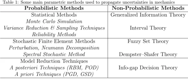
The deterministic structure has four tensile-compressive eigenmodes, and the associated eigenfrequencies were evaluated. The 99%-intervals presented in “Table 2” show the influence of stiffness uncertainties on the eigenfrequen-cies of the assembly. It can be noticed that the intervals are nearly identical and that the ones given by the LOK theory are included in the ones resulting from Monte Carlo simulations.
Figure 1: The 2D truss studied
Table 2: 99%-intervals for all the eigenfrequencies of the 2D truss (20000 samples)
i fi(Hz) MCS Perturbation SR LOK
1 276.4 [266.5 ; 285.8] [266.8 ; 286.0] [266.5 ; 285.8] [266.8 ; 285.6]
2 862.0 [834.3 ; 888.0] [835.0 ; 888.7] [834.3 ; 888.0] [835.8 ; 887.0]
3 1072.5 [1034.4 ; 1108.5] [1035.3 ; 1109.4] [1034.4 ; 1108.5] [1035.4 ; 1107.9] 4 1452.4 [1397.1 ; 1506.0] [1398.2 ; 1507.1] [1397.1 ; 1506.0] [1398.2 ; 1504.9]
An important question can then be asked whether the same accuracy can be obtained when considering a larger assembly, representative of a real industrial structure. The next study aims to provide an answer in this matter. 8.2. Second assembly
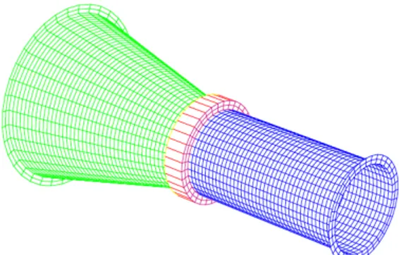
The assembly shown in “Figure 2” was inspired from the geometry of the booster pump studied in the framework of the international benchmark SICODYN [50, 51]. The main goal of this benchmark was to measure the effective variability on structural dynamics computations and then quantify the confidence in numerical models used either in design purpose or in ex-pertise purpose and finally to ensure robust predictions. The structure is an assembly of a cone and a tube with a wedge between these two elements. The whole set is made of steel (E = 210 GPa, ρ = 7800 kg/m3) and the largest
side of the cone is clamped. The mesh is composed of 3240 finite elements (∼20000 DOFs), which seems representative of industrial components.
In this case, the quantities of interest were the first three eigenfrequencies of the assembly. “Figure 3” shows the shapes of the corresponding eigenmodes for the reference structure and “Table 3” gives the 99%-intervals resulting from the statistical study of uncertainty propagation.
Figure 2: Mesh of the studied assembly
(a) Mode 1 (tensile-compressive):
211.69 Hz (b) Mode 2 (torsion): 699.28 Hz (c) Mode 3 (bending): 760.76 Hz
Figure 3: The shapes of the first three eigenmodes of the deterministic 3D assembly
The Monte Carlo method was considered as reference for the comparative analysis of the methods in terms of quality of the results. For that purpose, “Table 3” shows the highest algebraic percent error for both interval bounds and the central processing unit (CPU) computation time.
Table 3: 99%-intervals for the first three eigenfrequencies of the 3D assembly, with percent error and computation time (20000 samples)
i fi (Hz) MCS Perturbation SR LOK
1 211.69 [203.7 ; 219.4] [203.8 ; 219.5] [203.7 ; 219.4] [203.7 ; 219.4]
2 699.28 [672.8 ; 724.3] [673.3 ; 724.8] [672.8 ; 724.3] [673.2 ; 724.2]
3 760.76 [732.0 ; 787.7] [732.6 ; 788.6] [732.0 ; 787.7] [733.2 ; 787.1]
Percent Error (%) Reference [+0.08 ; +0.07] [0.00 ; 0.00] [+0.16 ; -0.06]
CPU Time ∼27.13 h ∼1 min ∼1.93 h ∼1 min
The results show that all implemented methods converge to similar re-sults. The LOK theory seems to be less conservative than MC, leading to
reduced intervals. In addition, the LOK theory and the perturbation method reveal to be the best in terms of computation time with a substantial advan-tage compared to other methods. The more numerous the degrees of freedom of the studied model are, the greater this advantage will be.
9. Conclusion
This paper aimed to provide engineers with practical information on the main probabilistic methods used to model and propagate uncertainties in structural mechanics. A brief overview of probabilistic approaches and the LOK theory was presented. Four lightly intrusive methods, modeling and propagating parametric uncertainties differently, were used to evaluate eigen-frequencies of two different assemblies. In the case of small uncertainties on stiffness parameters, the comparative analysis presented accurate results with a significant difference in terms of computation time. MCS and model reduc-tion techniques are time consuming. Stochastic FE methods provide results more quickly but are relatively intrusive. As for the LOK theory, it globalizes all sources of uncertainties, related to data and model, and seems to be less conservative. This modeling technique bounds the quantity of interest in a stochastic interval. The main advantage is the low implementation and com-putation time which can be handy when modeling real industrial assemblies. In the framework of the SICODYN Project [50, 51], initiated in 2012 and carried out till 2016, the comparative analysis will be extended to the case of a booster pump studied within its industrial environment. One of the goals is to evaluate the ability of some methods, such as the LOK theory and the generalized probabilistic approach of uncertainties [52], to quantify, not only data uncertainties, but also model uncertainties, especially in the case of high values of uncertainties.
10. Acknowledgements
This work has been carried out in the context of the FUI 2012-2016 SICO-DYN Project (SImulations credibility via test-analysis COrrelation and un-certainty quantification in structural DYNamics). The authors would like to gratefully acknowledge the support of the FUI (Fonds Unique Intermin-istériel).
References
[1] H. G. Matthies, C. E. Brenner, C. G. Bucher, C. Guedes Soares, Un-certainties in probabilistic numerical analysis of structures and solids– Stochastic finite elements, Structural safety 19 (1997) 283–336.
[2] G. Schuëller, A state-of-the-art report on computational stochastic me-chanics, Probabilistic Engineering Mechanics 12 (1997) 197–321. [3] M. Grigoriu, Stochastic mechanics, International Journal of Solids and
Structures 37 (2000) 197–214.
[4] G. S. Fishman, Monte Carlo: Concepts, Algorithms and Applications, Springer-Verlag, 1996.
[5] M. Kleiber, T. D. Hien, The stochastic finite element method : basic perturbation technique and computer implementation., John Wiley & Sons, England, 1992.
[6] R. G. Ghanem, P. D. Spanos, Stochastic Finite Elements: A Spectral Approach, Springer-Verlag, 1991.
[7] K. Willcox, J. Peraire, Balanced model reduction via the proper orthog-onal decomposition, AIAA Journal 40 (2002) 2323–2330.
[8] F. Chinesta, P. Ladevèze, E. Cueto, A short review on model order reduction based on proper generalized decomposition, Archives of Com-putational Methods in Engineering 18 (2011) 395–404.
[9] D. Moens, M. Hanss, Non-probabilistic finite element analysis for para-metric uncertainty treatment in applied mechanics: Recent advances, Finite Elements in Analysis and Design 47 (2011) 4–16.
[10] O. Dessombz, F. Thouverez, J.-P. Laîné, L. Jézéquel, Analysis of me-chanical systems using interval computations applied to finite element methods, Journal of Sound and Vibration 239 (2001) 949–968.
[11] R. L. Muhanna, R. L. Mullen, Uncertainty in mechanics problems– interval-based approach, Journal of Engineering Mechanics 127 (2001) 557–566.
[12] J.-P. Merlet, Interval analysis for certified numerical solution of prob-lems in robotics, International Journal of Applied Mathematics and Computer Science 19 (2009) 399–412.
[13] F. Massa, K. Ruffin, T. Tison, B. Lallemand, A complete method for efficient fuzzy modal analysis, Journal of Sound and Vibration 309 (2008) 63–85.
[14] G. Quaranta, Finite element analysis with uncertain probabilities, Com-puter Methods in Applied Mechanics and Engineering 200 (2011) 114– 129.
[15] Y. Ben-Haim, Information-gap Decision Theory: Decisions Under Severe Uncertainty, 2nd edition ed., Academic Press, 2006.
[16] G. J. Klir, Uncertainty and information: foundations of generalized in-formation theory, John Wiley & Sons, 2005.
[17] H.-R. Bae, R. V. Grandhi, R. A. Canfield, An approximation approach for uncertainty quantification using evidence theory, Reliability Engi-neering & System Safety 86 (2004) 215–225.
[18] C. Soize, A nonparametric model of random uncertainties for reduced matrix models in structural dynamics, Probabilistic Engineering Me-chanics 15 (2000) 277–294.
[19] C. Soize, Maximum entropy approach for modeling random uncertainties in transient elastodynamics, The Journal of the Acoustical Society of America 109 (2001) 1979–1996.
[20] P. Ladevèze, G. Puel, T. Romeuf, Lack of knowledge in structural model validation, Computer Methods in Applied Mechanics and Engineering 195 (2006) 4697–4710.
[21] F. Louf, P. Enjalbert, P. Ladevèze, T. Romeuf, On lack-of-knowledge theory in structural mechanics, Comptes Rendus Mécanique 338 (2010) 424–433.
[22] M. Papadrakakis, A. Kotsopulos, Parallel solution methods for stochas-tic finite element analysis using Monte Carlo simulation, Computer Methods in Applied Mechanics and Engineering 168 (1999) 305–320.
[23] G. I. Schuëller, C. G. Bucher, U. Bourgund, W. Ouypornprasert, On efficient computational schemes to calculate structural failure probabil-ities, Probabilistic Engineering Mechanics 4 (1989) 10–18.
[24] R. Caflisch, Monte Carlo and quasi-Monte Carlo methods, Acta numer-ica 7 (1998) 1–49.
[25] G. Blatman, B. Sudret, M. Berveiller, Quasi random numbers in stochas-tic finite element analysis, Mechanics & Industry 8 (2007) 289–298. [26] J. C. Helton, F. J. Davis, Latin hypercube sampling and the propagation
of uncertainty in analyses of complex systems, Reliability Engineering & System Safety 81 (2003) 23–69.
[27] O. Ditlevsen, H. O. Madsen, Structural Reliability Methods, volume 178, John Wiley & Sons, 1996.
[28] B. Huang, X. Du, Probabilistic uncertainty analysis by mean-value first order saddlepoint approximation, Reliability Engineering & System Safety 93 (2008) 325–336.
[29] B. Sudret, A. Der Kiureghian, Stochastic finite element methods and reliability: a state-of-the-art report, Department of Civil and Environ-mental Engineering, University of California, 2000.
[30] G. Stefanou, The stochastic finite element method: past, present and future, Computer Methods in Applied Mechanics and Engineering 198 (2009) 1031–1051.
[31] C.-C. Li, A. Der Kiureghian, Optimal discretization of random fields, Journal of Engineering Mechanics 119 (1993) 1136–1154.
[32] B. Van den Nieuwenhof, J.-P. Coyette, Modal approaches for the stochastic finite element analysis of structures with material and ge-ometric uncertainties, Computer Methods in Applied Mechanics and Engineering 192 (2003) 3705–3729.
[33] M. Shinozuka, G. Deodatis, Response variability of stochastic finite element systems, Journal of Engineering Mechanics 114 (1988) 499– 519.
[34] F. Yamazaki, M. Shinozuka, G. Dasgupta, Neumann expansion for stochastic finite element analysis, Journal of Engineering Mechanics 114 (1988) 1335–1354.
[35] M. Papadrakakis, V. Papadopoulos, Robust and efficient methods for stochastic finite element analysis using Monte Carlo simulation, Com-puter Methods in Applied Mechanics and Engineering 134 (1996) 325– 340.
[36] D. Xiu, G. E. Karniadakis, The Wiener–Askey polynomial chaos for stochastic differential equations, SIAM Journal on Scientific Computing 24 (2002) 619–644.
[37] G. Blatman, B. Sudret, Adaptive sparse polynomial chaos expansion based on least angle regression, Journal of Computational Physics 230 (2011) 2345–2367.
[38] A. Doostan, R. G. Ghanem, J. Red-Horse, Stochastic model reduction for chaos representations, Computer Methods in Applied Mechanics and Engineering 196 (2007) 3951–3966.
[39] D. Ryckelynck, A priori hyperreduction method: an adaptive approach, Journal of Computational Physics 202 (2005) 346–366.
[40] G. Rozza, D. Huynh, A. T. Patera, Reduced basis approximation and a posteriori error estimation for affinely parametrized elliptic coercive partial differential equations, Archives of Computational Methods in Engineering 15 (2008) 229–275.
[41] E. Balmès, Efficient sensitivity analysis based on finite element model reduction, in: Proc. IMAC XVII, SEM, Santa Barbara, CA, 1998, pp. 1168–1174.
[42] A. Nouy, A priori model reduction through proper generalized decom-position for solving time-dependent partial differential equations, Com-puter Methods in Applied Mechanics and Engineering 199 (2010) 1603– 1626.
[43] F. Chinesta, A. Ammar, A. Leygue, R. Keunings, An overview of the proper generalized decomposition with applications in computational
rheology, Journal of Non-Newtonian Fluid Mechanics 166 (2011) 578– 592.
[44] A. Nouy, O. P. Le Maître, Generalized spectral decomposition for stochastic nonlinear problems, Journal of Computational Physics 228 (2009) 202–235.
[45] F. Louf, L. Champaney, Fast validation of stochastic structural models using a PGD reduction scheme, Finite Elements in Analysis and Design 70–71 (2013) 44–56.
[46] F. Chinesta, A. Ammar, E. Cueto, Recent advances and new challenges in the use of the proper generalized decomposition for solving multidi-mensional models, Archives of Computational Methods in Engineering 17 (2010) 327–350.
[47] C. Soize, Random matrix theory for modeling uncertainties in com-putational mechanics, Computer Methods in Applied Mechanics and Engineering 194 (2005) 1333–1366.
[48] C. Soize, Generalized probabilistic approach of uncertainties in compu-tational dynamics using random matrices and polynomial chaos decom-positions, International Journal for Numerical Methods in Engineering 81 (2010) 939–970.
[49] P. Ladevèze, G. Puel, T. Romeuf, On a strategy for the reduction of the lack of knowledge (LOK) in model validation, Reliability Engineering & System Safety 91 (2006) 1452–1460.
[50] S. Audebert, SICODYN international benchmark on dynamic analysis of structure assemblies: variability and numerical-experimental correlation on an industrial pump, Mechanics & Industry 11 (2010) 439–451. [51] S. Audebert, A. Mikchevitch, I. Zentner, SICODYN international
benchmark on dynamic analysis of structure assemblies: variability and numerical-experimental correlation on an industrial pump (part 2), Me-chanics & Industry 15 (2014) 1–17.
[52] A. Batou, C. Soize, S. Audebert, Model identification in computational stochastic dynamics using experimental modal data, Mechanical Sys-tems and Signal Processing 50-51 (2015) 307–322.