Biosphere-climate interactions in current and future climate over North America

BIOSPHERE-CLIMATE INTERACTIONS IN CURRENT AND FUTURE CLIMATE OVER NORTH AMERICA

THESIS PRESE TED

AS PARTIAL REQ UIREME T

FOR PHD DEGREE IN EARTH AND ATMOSPHERIC SCIE CES

BY

CAMILLE GARNAUD

Avertissement

La diffusion de cette thèse se fait dans le respect des droits de son auteur, qui a signé le formulaire Autorisation de reproduire et de diffuser un travail de recherche de cycles supérieurs (SDU-522 - Rév.01-2006). Cette autorisation stipule que «conformément à l'article 11 du Règlement no 8 des études de cycles supérieurs, (l'auteur] concède à l'Université du Québec à Montréal une licence non exclusive d'utilisation et de publication de la totalité ou d'une partie importante de (son] travail de recherche pour des fins pédagogiques et non commerciales. Plus précisément, (l'auteur] autorise l'Université du Québec à Montréal à reproduire, diffuser, prêter, distribuer ou vendre des copies de [son] travail de recherche à des fins non commerciales sur quelque support que ce soit, y compris l'Internet. Cette licence et cette autorisation n'entraînent pas une renonciation de [la] part [de l'auteur] à [ses] droits moraux ni à [ses] droits de propriété intellectuelle. Sauf entente contraire, [l'auteur] conserve la liberté de diffuser et de commercialiser ou non ce travail dont [il] possède un exemplaire.»

INTERACTIONS BIOSPHÈRE-CLIMAT DANS LE CLIMAT RÉCENT ET

FUTUR EN AMÉRIQUE DU NORD

THÈSE

PRÉSENTÉE

COMME EXIGE CE PARTIELLE

DU DOCTORAT EN SCIENCES DE LA TERRE ET DE L'ATMOSPHÈRE

PAR

CAMILLE GARNAUD

l'aide compétente qu'elle m'a apportée, pour sa patience et son encouragement. Je re-mercie également Katja Winger et Luis Duarte sans qui je n'aurais pu accomplir cette thèse. Merci aussi à Vivek Arora pour m'avoir fournis CTEM, ainsi que l'aide nécessaire pour comprendre ce modèle.

Je remercie enfin tous ceux du Centre ESCER et de l'UQAM qui, d'une manière ou d'une autre, ont contribué à la réussite de ce travail et qui ne sont pas cités ici.

Enfin, faire une thèse, c'est aussi soutenir et être soutenue par la tribu des doctorants et autres chercheurs : Danahé, Fred, Jacinthe, Guillaume, Jean-Philippe et les autres membres de cette communauté que j'oublie de citer. Merci pour ces heures de diner à discuter de tout et de rien, pour votre soutien depuis mon arrivée au Qu 'b c et tout particulièrement pour votre soutien dans cette période éprouvante qu'est la dernière ligne droite.

Une thèse est impossible sans un soutien affectif; la famille en constitue la meilleure source. Sans elle, je n'aurais certainement pas tenu durant toutes ces années. Je tiens donc à remercier chaudement mes parents qui m'ont permis de faire les études que je voulais, où je voulais. Un bel héritage que j'espère transmettre à mes 2 filles! Mes filles, Juliette et Emma, qui m'ont soutenues sans le savoir durant ce doctorat lorsqu'elles dansaient la samba dans ma bedaine. Merci les filles, vous êtes mes bulles d'oxygène, mon équilibre, surtout en cette fin de doctorat! And last but certainly not least, des remerciements émus à mon conjoint, Sébastien, pour son amour et son soutien infaillible tout au long de mes études. Sans ma famille, je n'en serais pas là et je leur dédie cette thèse.

Quoique l'UQAM soit une institution de langue française, cette thèse est présentée en anglais afin d'élargir le bassin de lecteurs et de réviseurs externes. Je présente mes sincères excuses aux lecteurs de cet ouvrage pour qui ce pourrait être problématique.

LIST OF ACRONYMS XV

RÉSUMÉ .. XV!l

ABSTRACT XlX

INTRODUCTION 1

CHAPTER 1

THE EFFECT OF DRIVING CLIMATE DATA ON THE SIMULATED TER-RESTRIAL CARBON POOLS AND FLUXES OVER NORTH AMERICA 7 1.1 Introduction . . . . . . . . . . . . . . . . . . . 8

1.2 Models, Experimental Set-up and Data Sets . 10

1.2.1 Coupled land surface and terrestrial ecosystem models . 1.2.2 Experimental set-up . .

1.2.3 Data sets and methods 1.3 Results and Discussion . . . . .

1.3. l Driving data validation

1.3.2 CLASS/CTEM evaluation and analysis

1.4 Summary and Conclusions . . . . . . . . . CHAPTER II

IMPACT OF DYNAMIC VEGETATION ON THE CANADIAN RCM SIMULA-10 12 14 17 17 19 30

TED CLIMATE OVER NORTH AMERICA 35

2.1 Introduction . . . . . . . . . . . 36

2.2 Model, Experiments and Methods 39

2.2.1 The Canadian Regional Climate Model 2.2.2 Experiments . . . . . . . . . . .

2.2.3 Methods of model output evaluation and analysis .

39 41 46

2.3 Results and Discussion . . . . 2.3.1 CRCM5_STAT evaluation

2.3.2 Mean climate : CRCM5_STAT vs. CRCM5_DYN

48

48

2.3.4 Interannual variability and extremes 62

2.4 Summary and Conclusions . . . 68 CHAPTER III

BIOSPHERE-CLIMATE INTERACTIONS IN A CHANGING CLIMATE OVER

NORTH AMERICA 71

3.1 Introduction. . . . . 72

3.2 Models, Experiments and Methods 74

3.2.1 The Canadian Regional Climate Model (CRCM5) 3.2.2 Transient climate experiments

3.2.3 Methods of analysis 3.3 Results and Discussion . . .

3.3.1 Performance and boundary forcing errors 3.3.2 Projected changes to biosphere characteristics . 3.3.3 Impact of the biosphere on future climate . .. 3.3.4 Evolution of biosphere-atmosphere correlations 3.4 Summary and Conclusions .

CONCLUSION . REFERENCES . 74 76 79 80 80 83

87

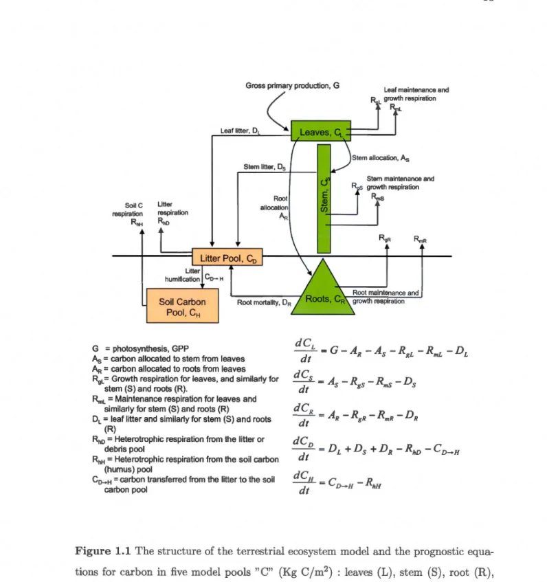
1.1 The structure of the terrestrial ecosystem model and the prognostic equ a-tions for carbon in five model pools "C" (Kg C/m2_{) : leaves (L), stem} (S), root (R), litter or debris (D), and soil organic matter or humus (H). 13 1.2 The manner in which the land surface scheme CLASS and the terrestrial

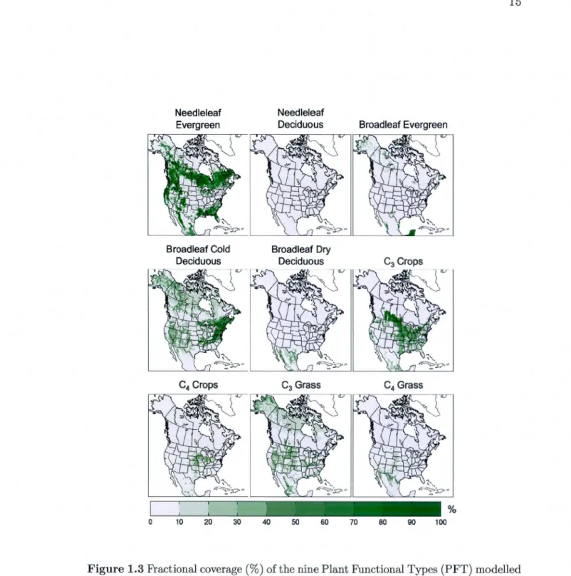
ecosystem module CTEM are coupled to each other. CTEM sub-modules are shown with a thick dark outline. . . . . . . . . . . . . . . . . . . 14 1.3 Fractional coverage (%) of the nine Plant Functional Types (PFT)

mo-delled by CTEM for the North American domain.. . . . . . . . . . . . . 15 1.4 Difference between the 1958-2001 NCEP and ERA40 (a) precipitation

(mm/day) and (b) mean air temperature (°C) and that of CRU for the winter (DJF) and summer (JJA) periods. . . . . . . . . . . . . . . . 18 1.5 The spatial plots correspond to the mean annual (a) GPP (kgC.m-2_{.yr-1 )}

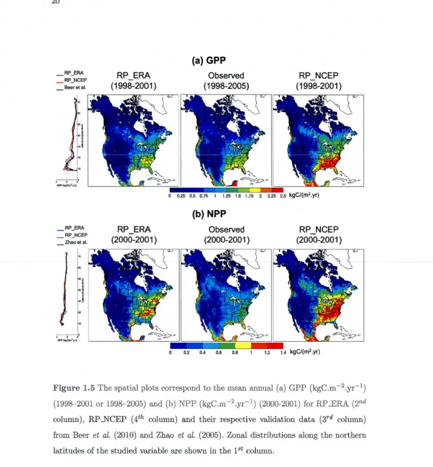
(1998-2001or1998-2005) and (b) NPP (kgC.m-2.yr-1) (2000-2001) for RP_ERA (2nd column), RP ...NCEP (4th column) and their respective va-lidation data (3rd column) from Beer et al. (2010) and Zhao et al. (2005). Zonal distributions along the northern latitudes of the studied variable are shown in the 1 st column. . . . . . . . . . . . . . . . . . . . . . . 20 1.6 The spatial plots correspond to the mean annual (a) woody biornass

(kgC/m2) (1995-1999) and (b) green LAI (m2 /m2) (1995-1998) for RP _.ERA (2nd column), RP _NCEP (4th column) and their respective validation data (3rd column) from Dong et al. (2003) and from ISLSCP II (Los et al., 2000; Hall et al., 2006; Sietse, 2010). Zonal distributions along the northern latitudes of the studied variable are shown in the 1 st column. . 22 1.7 Mean annual Carbon Use Efficiency (NPP /GPP) during the 1990-1999

period for RP _.ERA (top left; spatial mean = 0.573), RP _NCEP (top right; spatial mean = 0.585) and the CUE calculated using NPP esti-mates from Zhao et al. (2005) and GPP estimates from Beer et al. (2010) (bottom left), and using both NPP and GPP estimates from Zhao et al. (2005) (bottom right). . . . . . . . . . . . . . . . . . . . . . 26

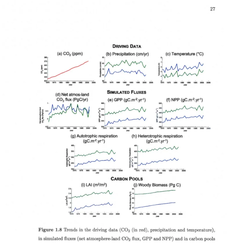
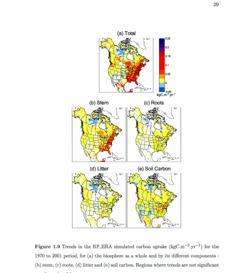
1.8 Trends in the driving data (C02 (in red), precipitation and temperature), in simulated fluxes (net atmosphere-land C02 flux, GPP and NPP) and in carbon pools (LAI, woody biomass and soil carbon mass) over the study domain from 1970 to 2001 for the RP __ERA simulation (in blue) and the RP _NCEP (in green) simulations. . . . . . . . . . . . . 27 1.9 Trends in the RP ..ERA simulated car bon uptake (kgC.m- 2 .yr-1_{) for the}

1970 to 2001 period, for (a) the biosphere as a whole and by its different components : (b) stem, (c) roots, (d) litter and (e) soil carbon. Regions where trends are not significant are shown in white. . . . . . . . . . 29

1.10 Trends in the RP _NCEP simulated carbon uptake (kgC.m- 2.yr-1

) for the 1970 to 2001 period, for (a) the biosphere as a whole and by its different components : (b) stem, (c) roots, (d) litter and (e) soil carbon. Regions where trends are not significant are shown in white. . . . . . . . 31

1.11 Trends in the net primary productivity (NPP, in gC.m-2 .yr-2) for the 1970- 2001 period for grid-cells where trends are significant at a:

=

53

2.1 Schematic diagram demonstrating the representation of vegetation PFTs in (a) CRCM5_STAT and (b) CRCM5..DYN simulations. The interactions between CTEM and CLASS are also shown in CRCM5_DYN. PFT stands for Plant Functional Type, and LAI for Leaf Area Index . . . . . . . 41

2.2 Fractional coverage (%) of the nine Plant Functional Types (PFT) consi-dered in CTEM for the North American study domain . . . . . . . . . . 43

2.3 Differences in mean seasonal (a) temperature (°C) and (b) precipitation (mm/day) between CRCM5_STAT and CRU (columns 1 and 3) and bet-ween CRCM5_STAT and UDEL (columns 2 and 4) for the 1971-2010 period . . . . . . . . . . . . . . . . . . . . . . . . . . . . 49

2.4 Spatial plots of the mean (a) annual and (b) summer LAI (m2 /m2) (1982-1998) for CRCM5_STAT (1 st column), CRCM5_DYN (3rd column) and the ISLSCPII data (2nd column) . . . . . . . . . . . . . . . 50 2. 5 Differences in the annual ( 1 st column), spring (MAM ; 2nd column) and

summer (JJA; 3rd column) mean (a) precipitation (mm/day) and (b) temperatures (°C) between CRCM5..DYN and CRCM5_STAT for the 1971-2010 period . . . . . . . . . . . . . . . . . . . . . . . . . . . . . 52 2.6 Differences in mean seasonal (a) temperature (°C) and (b) precipitation

(mm/day) between CRCM5..DYN and CRU (columns 1 and 3) and bet-ween CRCM5_STAT and UDEL (columns 2 and 4) for the 1971-2010 period . . . . . . . . . . . . . . . . . . . . . . . . . . . . . . . . . . . . . 54

dent 's t-test at 5% significance level . . . . . . . . . . . . . . . . . . . . 55

2.8 Spatial plots of the correlations between the maximum LAI and mean spring/summer (a) precipitation, (b) LHF, (c) temperature, and (d) SHF for the 1971-2010 period. Regions where correlations are not significant are shown in white; significance is calculated using the Student's t-test at 10% significance level. Path analysis illustrating the direct, indirect and overall effects of (e) maximum LAI and SHF on temperature, and (f) maximum LAI and temperature (T) on SHF, in CRCM5_DYN in the region defined by the black box in (a) . . . . . . . . . . . . . . . . . . . 58

2.9 Spatial plots of 1-year lagged-correlations between (a) precipitation and peak LAI, (b) temperature and peak LAI, (c) peak LAI and prec ipita-tion, and ( d) peak LAI and temperature, with the first variable leading the second by one year in all cases, for CRCM5_STAT ( column 1) and CRCM5_DYN (column 2) for the 1971-2010 period. Regions where co r-relations are not significant are shown in white; significance is calculated using the Student's t-test at 10% significance level . . . . . . . . . . 60

2.10 Spatial plots of the coefficient of variation of the (a) maximum LAI and mean (b) latent heat flux, ( c) sensible heat flux, ( d) precipitation, ( e) tem-perature, and (f) diurnal temperature range for the CRCM5_STAT and CRCM5_DYN simulations, for the 1971-2010 period, for spring (MAM) season . . . . . . . . . . . . . . . . . . . . . . . . . . . . . . 63

2 .11 Spatial plots of the coefficient of variation of the (a) maximum LAI and mean (b) latent heat flux, (c) sensible heat flux, (d) precipitation, (e) temperature, and (f) diurnal temperature range for the CRCM5_STAT and CRCM5_DYN simulations, for the 1971-2010 period, for summer (JJA) season . . . . . . . . . . . . . . . . . . . . . . . . . . 64

2.12 Number of hot days derived from (centre) observed data (Canada: Hop-kinson et al., 2011 and USA : Maurer et al., 2002) daily maximum tem-perature series, and the (left) CRCM5_STAT and (right) CRCM5_DYN simulations during the summer (JJA) of 1988 . . . . . . . . . . . . . . . 66 2.13 Evolution of CRCM5_STAT (left column) and CRCM5_DYN (right

co-lumn) simulated mean summer (a) precipitation (cm), (b) temperature (°C) and (c) LAI (m2/m2) for the 1988 drought affected region (be t-ween 41°N and 50°N, and 116°W and 88°W) shown in Fig. 2.12, for the 1971-2010 period. The filled (empty) circles correspond to year 1988 (1993) 67

3.1 Differences between STAT _ERA and CRU (left) and DYN _ERA and CRU (right) mean summer (JJA) (a) temperature (°C) and (b) precipitation (mm/day) for the 1971-2000 period . . . . . . . . . . . . . . . . . . 81

3.2 Differences between DYN_RCP45 and DYN_ERA simulated mean sum-mer (JJA) (a) temperature (°C), (b) precipitation (mm/day), and (c) leaf area index (m2 _/m2

) for the 1971-2000 period . . . . . . . . . 82 3.3 A ver age julian day of leaf onset for broadleaf cold deciduous trees for (a)

current 1971-2000 period for DYN_RCP45, and future 2071-2100 period for (b) DYN_RCP45 and (c) DYN_RCP85 simulations. . . . . . . 84 3.4 Average value in current 1971-2000 period for DYN_RCP45 (lst column),

projected change in DYN_RCP45 (2nd column) and DYN_RCP85 (3rd column), and differences between DYN_RCP85 and DYN_RCP45 (4th column) in the future 2071-2100 period of the (a) gross primary pro-ductivity (GPP; kgC.m-2.yr-1 ), (b) net primary productivity (NPP; kgC.m-2_.yr-1_{), (c) maximum LAI (m}2_.m-2

) and (d) total vegetation biomass (kgC.m-2

) . . . • . . . 85

3.5 Trends in NPP (in gC.m-2_.yr-2

) for (a) 1971-2100, (b) 1971-2010, (c) 2011-2040, (d) 2041-2070 and (e) 2071-2100 periods for grid cells where trends are significant at a=5% significance level for the DYN_RCP45

(left) and DYN_RCP85 (right) simulations. . . . . . . . . . . . . . . . . 86

3.6 Summer (JJA) mean temperature (0

C) for (a) projected change by 2071-2100 in STAT_RCP45 (lst column) and DYN_RCP45 (2nd column), and their differences (3rd column), and (b) projected change by 2071-2100 in STAT_RCP85 (lst column) and DYN_RCP85 (2nd column), and their differences (3rd column). . . . . . . . . . . . . . . . . . . 88

3.7 Summer (JJA) precipitation (mm/day) for (a) projected change by 2071-2100 in STAT_RCP45 (lst column) and DYN_RCP45 (2nd column), and their differences (3rd column), and (b) projected change by 2071-2100 in STAT_RCP85 (lst column) and DY _RCP85 (2nd column), and their differences (3rd column). . . . . . . . . . . . . . . . . . . . . . 89

3.8 Spatial plots of the correlations between the annual maximum LAI and mean spring/summer (MAMJJA) temperature for the current 1971-2000 and future 2071-2100 periods for (a) STAT_RCP45 and STAT_RCP85 and (b) DYN_RCP45 and DYN_RCP85. Regions where correlations are not significant are shown in white; significance is calculated using the Student's t-test at 10% significance level . . . . . . . . . . . . . . . . . . 91

in white; significance is calculated using the Student's t-test at 10% si-gnificance level . . . . . . . . . . . . . . . . . . . . . . . . . . . . . . . . 92

1.1 Coefficient of determination (R2

) and root mean square error (RMSE) values from the NPP and GPP values against the respective evaluation data for both RP _ERA and RP _NCEP simulations. . 21 3.1 Experimental setup and names given to simulations. 77

CGCM CLASS CRCM5 CTEM CUE DVM GHG GPP LAI LHF NA NPP PFT RCM RCP SHF SST WUE

Coupled Global Climate Model Canadian LAnd Surface Scheme

Canadian Regional Climate Model, 5th generation Canadian Terrestrial Ecosystem Model

Carbon Use Efficiency Dynamic Vegetation Model GreenHouse Gases

Gross Primary Productivity Leaf Area Index

Latent Heat Flux North America

Net Primary Productivity Plant Functional Type Regional Climate Model

Representative Concentration Pathway Sensible Heat Flux

Sea Surface Temperature Water Use Efficiency

sur la terre, la végétation affecte le climat à travers la modification des caractéristiques physiques de la surface de la terre. La plupart de nos connaissances sur ces interac-tions bi-directionnelles sont basées sur des modèles climatiques en raison d'un manque d'observations. Cependant, du fait de leur faible ré olution, les modèles climatiques glo-baux peuvent négliger un certain nombre d'interactions biosphère-atmosphère à l'échelle régionale et locale. L'objectif principal de cette thèse est donc d'étudier la var iabi-lité spatio-temporelle des interactions et rétroactions biosphère-atmosphère à l'échelle régionale, plus particulièrement en Amérique du Nord, en utilisant la cinquième géné-ration du Modèle Régional Canadien du Climat (MRCC5), qui comprend le modèle de végétation dynamique CTEM ( Canadian Terres trial Ecosystem Mo del).

La première partie de la thèse porte sur la validation du modèle de végétation dynamique CTEM couplé au Canadian Land Surface Scheme (CLASS) à travers des simulations découplées du modèle climatique sur l'Amérique du Nord. Sachant bien que des biais dans les données de forçage pourraient avoir une incidence sur la biosphère simulée par CTEM/CLASS, deux réanalyses différentes sont utilisées pour forcer le modèle. Les deux variables les plus importantes vis-à-vis de leur influence sur la végétation sont les précipitations et la température. Ainsi, leurs différences entre les deux ensembles de données de forçage ont un impact bien marqué sur les différents réservoirs et des flux de carbone simulés, en particulier sur l'est de l'Amérique du Nord. Cependant, malgré des flux bruts très différents, le modèle produit des estimations similaires de flux net de C02 entre la terre et l'atmosphère avec les deux ensembles de données de forçage. L'analyse de la distribution spatiale de l'évolution des stocks et des flux de carbone simulés montre que le puits de carbone simulé en Amérique du Nord est principalement attribuable aux augmentations de la productivité nette dans l'est des États-Unis, également rapporté par d'autres études, renforçant ainsi la confiance dans le modèle.

La deuxième partie de la thèse porte sur l'évaluation de l'impact de la végétation dyna-mique, soit CTEM, sur le climat simulé par le MRCC5 en Amérique du Nord pour la période 1971-2010. Deux simulations du MRCC5, avec et sans CTEM, sont analysées en accordant une attention particulière aux interactions biosphère-atmosphère et sa va-riabilité spatio-temporelle. L'analyse montre que la végétation dynamique améliore les interactions à l'interface terre-atmosphère, ce qui se reflète dans les fortes corrélations entre la biosphère et les variables atmosphériques. De même, le MRCC5 incluant la végétation dynamique démontre une mémoire à long terme, mise en évidence par des corrélations en décalage, et une amélioration de la variabilité interannuelle, reflétée dans

les états de la biosphère et l'atmosphère durant les années anormalement sèches ou hu-mides.

Enfin, la troisième partie de la thèse porte sur les modification prévues dans les interac-tions biosphère-climat, et explore la contribution de la végétation dynamique aux chan-gements climatiques. Cette étude utilise des simulations de l'évolution climatique, avec et sans CTEM, couvrant la période 1971-2100 et forcées aux frontières par le Canadian Earth System Model (CanESM2), et qui correspondent à deux scénarios d'émissions futures - RCP4.5 et RCP8.5. L'augmentation du C02 et des températures conduisent à une augmantation de la productivité et de la biomasse de la végétation, et à renfor-cer l'efficacité d'utilisation de l'eau de la végétation dans le climat futur. De plus, la végétation dynamique permet à la biosphère simulée de répondre aux modifications du climat par une série de rétroactions qui, à leur tour, contribuent de manière significative au changement climatique.

La recherche ci-dessus contribue ainsi à une compréhension systématique de la valeur ajoutée de la végétation dynamique dans le MRCC5 ainsi que la nature et la variabilité des interactions biosphère-atmosphère sur l'Amérique du Nord dans le climat r 'cent et futur.

Mots-clés : végétation dynamique, modélisation climatique régionale, interactions bio-sphère-climat

surface. Most of our current understanding of these bi-directional interactions is based on climate models, due to lack of observations. There is again the limitation that most of the global climate models used to study these bi-directional interactions are of coarse resolution and thus can overlook regional to local interactions. The main aim of this thesis therefore is to study spatio-temporal variability of biosphere-atmosphere interac-tions and feedbacks at regional scale, more specifically over North America, using the fifth generation of the Canadian Regional Climate Madel (CRCM5), which includes the dynamic vegetation model CTEM ( Canadian Terrestrial Ecosystem Mo del).

The first part of the thesis focuses on validating the dynamic vegetation model CTEM coupled to the Canadian Land Surface Scheme (CLASS) through offiine simulations over North America. Knowing well that biases in the driving data could impact CLASS/ CTEM simulated biosphere, two different reanalysis products are used to drive the mo-del. The differences in precipitation and temperature, the two most important climate variables that impact vegetation, in these two driving datasets are reflected in most of the simulated carbon pools and fluxes, particularly over eastern North America. Howe-ver, despite very different gross fluxes, the model yields fairly similar estimates of the net atmosphere-land C02 flux when driven with the two forcing datasets. The analysis of the spatial distribution of trends in simulated car bon pools and fluxes shows that the simulated carbon sink over North America is driven primarily by net productivity en-hancements over eastern United States, as reported by other studies, once again giving confidence in the model.

The second part of the thesis focuses on assessing the impact of dynamic vegetation, i.e. CTEM, on the CRCM5 simulated climate over North America for the 1971-2010 period. This is achieved by comparing two CRCM5 simulations, with and without CTEM, paying special attention to biosphere-atmosphere interactions and its spatio-temporal variability. Analysis shows that dynamic vegetation improves interactions at the land-atmosphere interface, which is reflected in the high correlations between biospheric and atmospheric variables. Similarly, CRCM5 with dynamic vegetation demonstrates long-term memory, estimated through lag correlations, and improved interannual variability, reflected in the biosphere and atmosphere states for anomalously dry and wet years. Finally, the third part of the thesis studies projected changes to biosphere-climate in-teractions, and explores the contribution of vegetation dynamics to climate change. Transient climate change experiments, spanning the 1971-2100 period, driven by the

Canadian Earth System Model at the lateral boundaries, corresponding to two future emission scenarios - RCP4.5 and RCP8.5, with and without CTEM, are employed. Results show that increased C02 and temperatures lead to increased vegetation pro-ductivity and biomass, and enhanced vegetation water use efficiency in future climate. Furthermore, as dynamic vegetation allows biosphere to respond to climate change, it significantly modulates future climate, and therefore climate change, through thermal and hydrological feedbacks.

The above research thus contributes to a systematic understanding of the added value of dynamic vegetation in CRCM5 as well as the nature and variability of biosphere-atmosphere interactions over North America in current and future climates.

Keywords : dynamic vegetation, regional climate modelling, biosphere-climate interac-tions

components of the Earth System constitute the most comprehensive tools to study climate change and variability. However, because of the high complexity of the climate system and because the physical processes occurring within each of its components cover a wide range of temporal and spatial scales, GCM simulations are very demanding in computational resources and are thus performed at coarse horizontal resolution. Low resolution precludes GCMs from resolving adequately key regional and local climate processes. Hence, Regional Climate Models (RCMs) have been increasingly employed to dynamically downscale CGCM simulations to finer scales over a region of interest,

allowing for high resolution without an increase in computational cost (Laprise, 2008; Rummukainen, 2010). At the resolution of the RCMs, regional water bodies and land-surface heterogeneities begin to be explicitly resolved, thus allowing realistic feedback processes that will increase the realism of climate simulations.

Several studies have demonstrated the importance of the land surface, and particularly the biosphere, in the climate system (Betts et al., 1996; Pielke et al., 1998; Bonan, 2008). Land surface controls the energy and water partitioning at the surface (Brovkin, 2002; Notaro et al., 2006) and is also important from the point of view of carbon exchanges and thus plays an important role in the terrestrial carbon storage evolution. It can therefore influence the climate on time scales ranging from seconds to thousands of years, particularly in transient climate conditions.

Land Surface Models (LSMs) have therefore been developed to include key processes of exchanges of energy, water, momentum and car bon between the surface and the at-mosphere in climate models (Pitman, 2003; Bonan, 2008). The first generation of LSMs used simple aerodynamic bulk transfer equations and simple prescriptions of albedo,

surface roughness, and soil water without explicitly representing vegetation or the hy-drological cycle (Manabe, 1969). They have since evolved to simulate the hydrological and biogeochemical cycles and vegetation realistically (e.g. Friedlingstein et al., 1995; Cox et al., 1999). Climate models with LSMs of varying complexities have been used to understand the impact of changes in land surface characteristics and processes on climate. For instance, climate models with physically based LSMs have been employed to study impacts of deforestation on climate (e.g., Nobre et al., 1991; Snyder et al., 2004; Garcia-Carreras and Parker, 2011). However, such studies were performed with prescribed changes in vegetation cover because land surface models do not simulate long-term changes in the variability and the characteristics of the biosphere, which are crucial, particularly in the context of a changing climate.

Dynamic Vegetation Models (DVMs) have therefore been developed (e.g., Friend et al., 1995; Foley et al., 1996; Bonan et al., 2003; Hughes et al., 2006) in order to enable the simulation of large-scale structural vegetation changes in response to variations in climate and atmospheric C02 concentrations, and to incorporate the relevant biosphere-atmosphere feedback mechanisms in Earth System Models (Denman and et al., 2007). DVMs represent vegetation in terms of plant functional types (PFTs). This approach broadly classifies vegetation according to its form and fonction into functionally similar types (Box, 1996) such as broadleaf and needleleaf trees and their deciduous and ever-green types ; crops and grasses are separated into C3 and C4 types according to their photosynthetic pathways. This classification does not take into account species level differences that become important at local scales but is considered sufficient to capture continental scale variability in terrestrial carbon pools and fluxes. A DVM simulates

dif-ferent carbon pools, such as stems, roots, and leaves, and the changes in the terrestrial ecosystem, like vegetation structure and composition, which affect these pools.

Several DVMs have been developed for u e in climate models, such as TRIFFID (Cox, 2001), which is used in the Hadley Center GCM and the Lund-Potsdam-Jena Dynamic Global Vegetation Model (LPJ-DGVM; Sitch et al., 2003), which has been recently coupled to the Rossby Centre Regional Climate Model. The available DVMs all differ

models simulate a net carbon uptake by the end of the 21st century, the magnitude of the land uptake vary significantly amongst the DVMs, thus indicating large uncertainties in the terrestrial biosphere response to changing climatic conditions (Sitch et al., 2008). They conclude that though all models agree on the increased productivity of plants with increased atmospheric C02 concentrations, the carbon uptake simulated by a DVM is very dependent on the climate characteristics simulated by the climate model.

Jiang et al. (2012) analysed the uncertainties of vegetation distribution in the northern

high-latitudes using an ensemble of LP J-DGVM simulations under different SRES (Spe-cial Report on Emission Scenarios) scenarios. They found that the relative importance of different vegetation-related parameters, such as parameters that control plant car bon uptake and light-use efficiency, depend on the region and time of the year, and is greatly influenced by climate. The authors suggest that the uncertainties in vegetation distri-bution induced by vegetation-related parameters contribute significantly to the total

uncertainty, though climate-induced and emission-induced uncertainties are larger. The above studies, focusing on the uncertainties coming from DVMs, lead to the conclusion that more work is necessary in the simulation of the biosphere as part of the climate system.

The dynamic vegetation model CTEM (Canadian Terrestrial Ecosystem Model) was developed at the Canadian Centre for Climate modelling and analysis (CCCma) (Arora, 2003; Arora and Boer, 2003, 2005, 2006; Li and Arora, 2011), to serve as the carbon cycle component in the CCCma atmosphere-ocean GCM. CTEM is a process-based ecosystem model, and it is able to grow vegetation from bare ground and simulates several time-varying vegetation structural attributes including leaf area index, vegetation height, root distribution and canopy mass. It includes processes of photosynthesis, autotrophic and heterotrophic respiration, phenology, turnover, allocation, fire and land-use change. CTEM simulates two dead carbon pools, litter and soil organic carbon, and three live

vegetation pools (stems, leaves and roots), and as such CTEM is able to provide net fluxes of C02 between the land and the atmosphere. Terrestrial ecosystem processes in CTEM are modeled for nine different plant functional types (PFTs) ; evergreen and deciduous needleleaf trees, broadleaf evergreen and cold and drought deciduous trees, and C3 and C4 crops and grasses.

CTEM was designed to be coupled to the Canadian Land Surface Scheme (CLASS; Verseghy, 1991, 2011; Verseghy et al., 1993), and for this research, the coupled CLASS/ CTEM was implemented in the fifth generation Canadian Regional Climate Madel (CRCM5; Martynov et al., 2013; Separovic et al., 2013). This enables the study of biosphere-atmosphere interactions and their impact on the simulated climate at a hi-gher resolution (0.5°) than would be possible using a CGCM. Such high-resolution studies of biosphere-atmosphere interactions are especially lacking over North America, and hence the importance of the research presented in this thesis.

It is worth noting that observation-based studies of biosphere-atmosphere interactions are also on the rise, with biosphere related observations starting to become increasin-gly available, and this is well reflected in the published literature. For instance, Notaro

et al. (2006) and Wang et al. (2014) used observations, i.e. satellite-based fraction of photosynthetically active radiation (FPAR) and monthly climate data, to show that vegetation can substantially impact the atmosphere over North America. These stu-dies indicate that vegetation could alter the amplitude of climate change locally and regionally through various feedbacks, and hence the need for a better understanding of biosphere-atmosphere interactions and their impact on climate.

Scientific objectives and approach

The main objective of this research is to study biosphere-climate interactions over North America in current and future climates. The main tool used in this study is CRCM5 with the Canadian Terrestrial Ecosystem Mo del ( CTEM). 0 bservations are used w henever possible to support model results. The systematic approach adopted to achieve the

pools and fluxes over North America', represents a paper published in the peer-reviewed International Journal of Climatology. The focus of this chapter is on the validation of the dynamic vegetation model CTEM coupled to the Canadian Land Surface Scheme (CLASS) through offiine simulations over North America. Offiine CTEM/CLASS simu-lations driven by two different reanalysis products over North America are performed. Simulated terrestrial carbon pools and fluxes over North America are then compared with observation-based estimates. Chapter II, entitled 'Impact of dynamic vegetation on the Canadian RCM simulated climate over North America' and submitted to Cli-mate Dynamics, assesses the impact of dynamic vegetation, i.e. CTEM, on the CRCM5 simulated climate over North America for the 1971-2010 period. This is achieved by comparing two CRCM5 simulations, with and without CTEM, paying special attention to biosphere-atmosphere interactions and its spatio-temporal variability. In the third and final chapter, entitled 'Biosphere-climate interactions in a changing climate over North America', projected changes in climate and biosphere are evaluated, and the re-sulting contributions of vegetation dynamics to climate change and to future climate variability are explored. Transient climate change experiments, spanning the 1971-2100 period, driven by the Canadian Earth System Model (CanEMS2) at the lateral boun-daries, corresponding to two future emission scenarios - RCP4.5 and RCP8.5, with and without CTEM, are employed.

TERRESTRIAL CARBON POOLS AND FLUXES OVER NORTH AMERICA

This chapter is presented in the format of a scientific article that has been published

in the peer-reviewed journal International Journal of Climatology. The design of the

research and its performance together with the analysis of data and the redaction of this article are entirely based on my work, with the co-authors involved in the supervision of all these tasks. The detailed reference is :

Garnaud, C., Sushama, L. and Arora, V. K. (2014). "The effect of driving climate data

on the simulated terrestrial carbon pools and fluxes over North America". International Journal of Climatology, 34 : 1098-1110. DOI : 10.1002/joc.3748

Abstract

Dynamic vegetation models provide the ability to simulate terrestrial carbon pools and

fluxes and a useful tool to study how these are affected by climate variability and climate change. At the continental scale, the spatial distribution of climate, in particular tempe

-rature and precipitation, strongly determines surface vegetation characteristics. Mode! validation exercises typically consist of driving a model with observation-based climate

data and then comparing simulated quantities with their observation-based counte

r-parts. However, observation-based datasets themselves may not necessarily be consistent

with each other. Here, we compare simulated terrestrial carbon pools and fluxes over

North America with observation-based estimates. Simulations are performed using the

dynamic vegetation model CTEM ( Canadian Terres trial Ecosystem Mo del) cou pled to the Canadian Land Surface Scheme (CLASS) when driven with two reanalysis-based

climate datasets. The driving ECMWF reanalysis data (ERA40) and NCEP /NCAR

when compared to the observation-based Climate Research Unit (CRU) data. Most si-mulated carbon pools and fluxes show important differences, particularly over eastern North America, primarily due to differences in precipitation and temperature in the two reanalysis. However, despite very different gross fluxes, the model yields fairly similar estimates of the net atmosphere-land C02 flux when driven with the two forcing data-sets. The ERA40 driven simulation produces terrestrial pools and fluxes that compare better with observation-based estimates. These simulations do not take into account land use change or nitrogen deposition, both of which have been shown to enhance the land carbon sink over North America. The simulated sink of 0.5 Pg C/yr during the 1980s and 1990s is therefore lower than inversion-based estimates. The analysis of spa-tial distribution of trends in simulated carbon pools and fluxes shows that the simulated carbon sink is driven primarily by NPP enhancements over eastern United States.

1.1 Introduction

The spatial distribution of vegetation, and terrestrial carbon pools and fluxes, at the continental to global scales is governed primarily by climate in particular temperature and precipitation (Walter and Box, 1976; Woodward, 1987; Stephenson, 1990; Prentice et al., 1992). Terrestrial carbon fluxes are also sensitive to decadal and inter-annual variability in climate. Nemani et al. (2003) showed that a decreased cloud cover, and the resulting increase in solar radiation, led to an increase in net primary production in Amazon rain forests during the 1982-1999 period. Gobron et al. (2005) studied the impact of the 2003 drought on plant productivity in Europe using remote-sensing data. They found that the drought affected the growth of vegetation but that the effects of the drought were temporally limited. Zhao et al. (2011) studied the effect of changing climate on vegetation in the arid region of north-western China during 1982-2003 and noted an increase in productivity which was well correlated to precipitation increase during the growing season and the preceding winter.

The development of Dynamic Vegetation Models (DVMs) (e.g. Peng, 2000; Cramer et al., 2001; Cox, 2001; Quillet et al., 2010; den Roof et al., 2011) has allowed to model changes in vegetation structure in response to climate variability and climate change in Earth System Models. As the climate changes, a DVM can simulate the changes in structural vegetation attributes and its spatial distribution. Consequently, vegetation

fluxes affect the biogeochemical processes through carbon cycle feedbacks (Cox et al., 2000; Myneni et al., 2001; Foley et al., 2003). DVMs represent vegetation in terms of plant functional types (PFTs). This approach broadly classifies vegetation according to its form and fonction into functionally similar types (Box, 1996) such as broadleaf and needleleaf trees and their deciduous and evergreen types; crops and grasses are separated into C3 and C4 types according to their photosynthetic pathways. This classification does not take into account species level differences that become important at local scales but is expected to capture continental scale variability in terrestrial carbon pools and fluxes. DVMs are typically validated against observation-based estimates of terrestrial carbon pools and fluxes when driven with observation-based climate data. However, observation-based climate datasets themselves may not necessarily be consistent with each other with consequences for model validation. The objective of this paper is to study the effect of driving climate data on the simulated terrestrial carbon pools and fluxes over North America, a region that covers several climatic zones and consequently biomes, using the Canadian Terrestrial Ecosystem Model (CTEM) (Arora, 2003; Arora and Boer, 2003, 2005) coupled to the Canadian Land Surface Scheme (CLASS) (Verseghy, 1991, 2011; Verseghy et al., 1993). Coupled CLASS/CTEM are driven offiine at 0.5° ( rv45km) re-solution over North America using the European Centre for Medium range Weather Forecast's (ECMWF) ERA40 reanalysis (Uppala et al., 2005) and the National Centers for Environmental Prediction's NCEP /NCAR reanalysis I data (Kalnay et al., 1996) from 1958 to 2001. Both simulations, one driven by ERA40 data and the other driven by NCEP data, are then evaluated by comparing CLASS/CTEM simulated terrestrial carbon pools and fluxes to observation-based estimates.

CTEM has been validated at selected sites and different PFTs in earlier studies (Arora and Boer, 2005; Li and Arora, 2011) and also at the global scale when implemented in an earth system model (Arora et al., 2009) but coupled to earlier versions of CLASS.

The CLASS version 3.5. used here better simulates the hydraulic and thermal regimes by incorporating an improved treatment of soil evaporation, a new canopy conductance formulation, and an enhanced snow density and snow interception.

This paper is organised as follows. Section 1.2 of the paper gives a brief overview of the coupled land-surface and terrestrial ecosystem models, CLASS and CTEM, along with the description of the experimental set-up and the methodology. In section 1.3, the effect of different driving data sets on vegetation growth and productivity is analysed by comparing them with observed and modelled data. Section 1.3 also assesses the spatial and temporal evolution of the simulated biosphere in the recent past. A brief summary of the results and conclusions are given in section 1.4.

1.2 Models, Experimental Set-up and Data Sets

1.2. l Coupled land surface and terrestrial ecosystem models

The configuration used here is comprised of the Canadian Terrestrial Ecosystem Mo-del (CTEM) (Arora and Boer, 2005) coupled to the Canadian Land Surface Scheme (CLASS) (version 3.5) (Verseghy, 2011). In its standard formulation, CLASS uses three soil layers, 0.1 m, 0.25 m and 3.75 m thick, corresponding approximately to the depth influenced by the diurnal cycle, the rooting zone and the annual variations of tempera-ture, respectively (Paitras et al., 2011). CLASS includes prognostic equations for energy and water conservation for the three soil layers and a thermally and hydrologically dis

-tinct snowpack where applicable ( treated as a fourth variable-depth layer). The energy

balance and temperature calculations are performed over the three soil layers, but the

hydrological balance calculations are performed only for layers above the bedrock. In an

attempt to crudely mimic subgrid-scale variability, CLASS adopts a "pseudo-mosaic" approach and <livides each grid cell into a maximum of four sub-areas : bare soil, ve -getation, snow over bare soil and snow with vegetation. The energy and water balance calculations are first performed for each sub-area separately, and then averaged over the grid cell, using averaged structural attributes and physiological properties of the four

CTEM, these structural vegetation attributes are dynamically simulated by CTEM as a fonction of environmental conditions.

CTEM is a process-based ecosystem model (Arora, 2003; Arora and Boer, 2003, 2005, 2006; Li and Arora, 2011) designed to simulate terrestrial ecosystem processes. It is able to grow vegetation from bare ground and simulates several vegetation structural attri-butes including leaf area index, vegetation height, root distribution and canopy mass. It includes processes of photosynthesis, autotrophic and heterotrophic respiration, pheno-logy, turnover, allocation, fire and land-use change. The photo ynthesis submodule uses the biogeochemical approach as described by Farquhar et al. (1980) and Collatz et al. (1991, 1992). CTEM simulates two dead carbon pools (litter and soil organic carbon) and three live vegetation pools (stems, leaves and roots). The structure of CTEM is shown in Figure 1.1 along with the prognostic equations for carbon in the five model pools. Terrestrial ecosystem processes in CTEM are modelled for nine different plant functional types (PFTs); evergreen and deciduous needleleaf trees, broadleaf evergreen and cold and drought deciduous trees, and C3 and C4 crops and grasses. The vegetation structural attributes of CTEM's nine PFTs are averaged for four PFTs (needleleaf trees, broadleaf trees, crops and grasses) when they are passed to CLASS. Figure 1.2 shows the manner in which CLASS and CTEM are coupled to each other. CLASS and CTEM's photosynthesis sub-module, simulating the fast biophysical processes, such as photo-synthesis, canopy conductance and leaf respiration, operate at a 30-minute timestep while other biogeochemical processes are modelled at a daily timestep. Once coupled, CLASS and CTEM simulate energy, water and C02 fluxes across the land-atmosphere boundary. However, CTEM does not include the coupling of carbon with nitrogen and phosphorus cycles and so, nutrient limitation of photosynthesis is not explicitly mo-delled. Nevertheless, CTEM implicitly models nutrient limitation by "downregulating" photosynthesis as C02 increases using an empirical formulation that is calibrated on the

basis of plants grown in elevated and ambient C02 environments (Arora et al., 2009).

1.2.2 Experimental set-up

The coupled CLASS and CTEM models are run offiine over the North American do-main shown in Figure 1.3, at a horizontal resolution of 0.5 degrees and a timestep of 30 minutes. The input data required to run the model include the incident solar and

longwave radiation, 2-m air temperature, relative humidity, 10-m wind velocity, surface pressure and total precipitation. The soil texture information, i.e. percentagc of sand and clay, for the three layers (see Section 1.2.1) is specified from Webb et al. (1991). Finally, the fractional coverage of CTEM's nine PFTs (Fig. 1.3) for the 0.5° grid cells are specified from Arora and Boer (2010) who use the HYDE 2 crop area data set (Wang et al., 2006) to reconstruct historical land cover. The land cover is specified at its 1960 values, so land use change is not taken into account. It should be noted that, even though the geographical distribution of PFTs is fixed, the vegetation attributes (LAI, land-atmopshere C02 fluxes and car bon pools) are simulated as dynamic fonctions of driving climate.

Two simulations are performed with CLASS/CTEM models using different driving cli-mate data. The first uses ERA40 reanalysis data (Uppala et al., 2005), and the second uses NCEP reanalysis (Kalnay et al., 1996). ERA40 data is available for the 1957-2002 period at 2.5° ( rv250 km) resolution, while NCEP data is available for the 1948-present period at 200 km resolution. These two simulations driven by ERA40 and NCEP for the common 1958-2001 period are referred to as RP _ERA and RP ...NCEP, respectively. Initial conditions for prognostic variables in CLASS and CTEM (including structural vegetation attributes) for the RP -ERA and RP ...NCEP simulations are obtained by s pin-ning the model from zero vegetation for 400 years, driven by repeated 1958-1977 ERA40 and NCEP climate data, respectively. Similarly to the CMIP5 modelling protocol (Ta y-lor et al., 2009, 2012), a constant C02 concentration value corresponding to the year 1765 is used for the first 207 simulation years for the spin up, followed by transient C02

Stem litter, Ds SoilC respiration RhH Litter respiration R•o Litter Pool, Co Lilier humification Co-H Rool allocation AR Soil Carbon Pool, CH Root mortality, DR G = photosynthesis, GPP

As = carbon allocated to stem from leaves AR = carbon allocated to roots from leaves R

9L= Growth respiration for leaves, and similarly for stem (S) and roots (R).

RmL = Maintenance respiration for leaves and similarly for stem (S) and roots (R)

DL= leaf litter and similarly for stem (S) and roots (R)

Rho = Heterotrophic respiration from the litter or debris pool

RhH = Heterotrophic respiration from the soil carbon (humus) pool

Co-H

=

Stem allocation, As

Stem maintenance and R s growth respiration

Rms

Root maintenance and growth respiration dCL dt=G-AR -As -RgL -Rmr -DL dCs =Âs-Rgs-Rms-Ds dt dCR - - =AR -RgR -R,,,R -DR dt dCD dt=Dr +Ds +Dn -RhD -CD-H

Figure 1.1 The structure of the terrestrial ecosystem model and the prognostic e qua-tions for carbon in five model pools "C" (Kg C/m2) : leaves (L), stem (S), root (R),

CLASS transmittivity calculations Photosynthesis, leaf respiration, and canopy conductance

Surface energy and water balance

Daily-averaged values of canopy temperature, soil temperature, soli moisture and carbon uptake

LAI, vegetalion roughness height, root distribution, canopy mass, and fractional coverage of PFTs CTEM 1 Autotrophic respiration 1 Heterotrophic respiration Allocation Phenology Turnover, mortality Conversion of biomass to structural attributes 6t• 1 day

Figure 1.2 The manner in which the land surface scheme CLASS and the terrestrial ecosystem module CTEM are coupled to each other. CTEM sub-modules are shown with a thick dark outline.

concentrations corresponding to the years 1765 to 1957 for the remaining 193 years. The transient 1958-2001 simulations RP _ERA and RP _NCEP are forced with evolving C02 concentrations from the Mauna Loa Observatory (Keeling et al., 1976; Thoning et al., 1989). Because the soil carbon is much slower to reach equilibrium than any other carbon pool (Fig. 1.1), an accelerator is used to allow the soil carbon pool to reach e qui-librium at a similar rate as the vegetation and the litter, so that all car bon pools have stabilised within the first part of the spinup (constant C02).

1.2.3 Data sets and methods

While the reanalysis data provide the sub-daily resolution of meteorological data needed for driving the CLASS and CTEM models they are not "observation-based" in a strict sense. Thus, prior to studying the impact of the climate data on vegetation, the ERA40 and NCEP seasonal mean temperature and precipitation used to drive CLASS/CTEM are compared to the gridded observational-based data from the Climate Research Unit (CRU) (Mitchell and Jones, 2005). The CRU TS 2.1 data set covers the period

1901-0 Needleleaf Evergreen Broadleaf Cold Deciduous 10 20 30 40 Needleleaf Deciduous Broadleaf Dry Deciduous 50 60 70 Broadleaf Evergreen 80 90

Figure 1.3 Fractional coverage (%) of the nine Plant Functional Types (PFT) modelled by CTEM for the North American domain.

2002 and has a resolution of 0.5°. This comparison helps identify biases in the two reanalysis datasets.

The simulated terrestrial pools and fluxes are analysed by comparing green leaf area index (LAI), net primary productivity (NPP), gross primary productivity (GPP) and woody biomass with observation-based estimates and multi-model results from other

studies. The observation-based green leaf area index were obtained from the Interna -tional Land Surface Climatology Project Initiative (ISLSCP II) FASIR-adjusted NDVI Biophysical Parameter Fields measured by the satellite mounted AVHRR sensor (Los

et al., 2000; Hall et al., 2006; Sietse, 2010). These monthly global data are available

for the 1982-1998 period at 1°xl 0

resolution. The net primary production (NPP) data are from the MODIS NPP /GPP project (MODl 7) (Zhao et al., 2005), a part of the

NASA/EOS project. It is a continuous satellite-driven dataset available from 2000 to 2006 at 1-km resolution. The algorithm used in MOD17 is based on the original logic of Monteith, suggesting that NPP under non-stressed conditions is linearly related to

the amount of absorbed Photosynthetically Active Radiation (PAR) during the g

ro-wing season. The MO Dl 7 product also combines the complex effects of temperature,

water and radiation on the productivity and corrects the data contaminated by

cloudi-ness or severe aerosol. The gross primary production (GPP) data were obtained from

observation-based estimations of global GPP for the 1998-2005 period using eddy c

o-variance flux data and various diagnostic models from the Beer et al. (2010) study.

Finally, the woody biomass data are from an AVHRR GIMMS NDVI data set with an

8-km resolution and forest inventory data for stem wood volume (Dong et al., 2003).

An equation that relates the forest inventory data with the satellite NDVI data as a fonction of latitude, was developed and tested by Dong et al. (2003) in order to estimate

the woody biomass with a high resolution across the northern hemisphere in the early

1980s and the late 1990s. The observation-based and multi-model mean data used for

validation corne from different sources and need not necessarily be consistent with each

other.

and the statistical significance of these trends is estimated using the Mann-Kendall test (Kendall, 1975; Khaliq et al., 2009) at 5% significance level.

1.3 Results and Discussion

1. 3.1 Driving data validation

The seasonal mean temperature and precipitation differences between the two reanalysis and the CRU dataset for the period 1958-2001 are shown in Figure 1.4. For the winter precipitation, bath NCEP and ERA40 reanalysis show similar differences compared to the CRU. There are two main regions of underestimation: up to 5 mm/day on the West Coast and in the Canadian Rocky Mountains and up to 2 mm/day in southeast USA. The NCEP and ERA40 summer precipitation compare differently to the CRU data. NCEP tends to overestimate precipitation by up to 5 mm/day in southeast USA and Mexico and by 4 mm/day in Alaska. It underestimates summer precipitation in some parts of northeast Canada and northwest Mexico by up to 4 mm/day. ERA40 tends to generally underestimate summer precipitation, particularly over the USA, by 1 or 2 mm/day, but as high as up to 4 rnm/day in southeast USA and up to 5 mm/day in Mexico (Fig. l.4a). Overall, ERA40 precipitation appears to compare better with the CRU data set, especially during summer when most of the vegetation growth occurs. In Figure l.4b, ERA40 generally overestimates the seasonal mean winter temperature by 1 to 2°C in the southern half of North America, and by up to 10°C in the high-latitude regions of northwest Canada and Alaska. NCEP generally tends to underestimate the winter temperatures, especially in the highlands of western USA (up to 6°C). For sea-sonal mean summer temperature, ERA40 shows a constant overestimation of between 2 and 6°C that is enhanced over the high elevations in western US (up to 10°C). Similar to ERA40, NCEP tends to overestimate the temperatures in summer except along the

(a)

ERA40 - CRU NCEP - CRU

DJF -1 -2 -3 JJA -4 _-5

(b)

ERA40 - CRU NCEP - CRU

DJF 10 4 -2 -4 -6 JJA -8 -10

Figure 1.4 Difference between the 1958-2001 NCEP and ERA40 (a) precipitation (mm/day) and (b) mean air temperature (°C) and that of CRU for the winter (DJF) and summer (JJA) periods.

Simmons et al. (2004) have shown that there is a warm bias in the surface temperature in the middle and high latitudes, especially prior to the 1970s due to the lack of sate l-lite observations. Their study also showed that when comparing ERA40 to the NCEP reanalysis, ERA40 is closest to the CRU analysis for all but the earliest years (prior to 1967).

1.3.2 CLASS/CTEM evaluation and analysis

The simulated terrestrial carbon pools and fluxes from the offline CLASS and CTEM simulations (RP _ERA and RP _NCEP) for the 1958-2001 period are compared with observations where possible and also analysed to investigate the trends for the 1970 -2001 period.

1.3.2.1 Evaluation of the mean state

Simulated NPP, GPP, woody biomass and green LAI, are compared with observa tion-based where available or with multi-model mean data as described in section 1.2.3. In Figure l.5a, RP _ERA GPP compares reasonably well with the observation-based es -timate from Beer et al. (2010). The model captures the spatial distribution of GPP relatively well, with high values located mostly in southeast US and along the coasts of Mexico. The rnodel also somewhat captures the high GPP values along the West Coast. The simulated higher GPP for the RP _NCEP case over southeast US is the result of hi-gher summer precipitation in the NCEP reanalysis (Figure 1.4a). While simulated GPP compares well with its observation-based estimate, simulated NPP for the RP _ERA case (Figure l.5b) is higher over the eastern US and generally low elsewhere when compa-red to the satellite-based NPP from MODIS (Zhao et al., 2005). Similar to GPP, NPP for the RP _NCEP case is too high compared to the estimate from Zhao et al. (2005), especially over eastern US, again due to higher than observed summer precipitation.

_ RP_ERA _ RP_NCEP Beeret al. _ RP_ERA _ RP_NCEP Zhao et al. "

.

Figure 1.5 The spatial plots correspond to the mean annual (a) GPP (kgC.m-2.yr-1) (1998-2001or1998-2005) and (b) NPP (kgC.m-2.yc1_{) (2000-2001) for RP _ERA (2nd} column), RP _NCEP (4th column) and their respective validation data (3rd column) from Beer et al. (2010) and Zhao et al. (2005). Zonal distributions along the northern

RP_ERA 0.5630 0.2924 0.6716 0.4392

Table 1.1 Coefficient of determination (R2) and root mean square error (RMSE) values from the NPP and GPP values against the respective evaluation data for both RF _ERA and RP _NCEP simulations.

CTEM uses a single-leaf photosynthesis approach and the coupling between photosyn-thesis and canopy conductance is based on vapour pressure deficit (Leuning, 1995). The effect of water stress on maximum potential temperature-based photosynthetic rate is taken into account by reducing the potential photosynthetic rate via a non-linear soil moisture fonction, which takes into account the degree of soil saturation, the wilting point and the field capacity soil moisture contents and the fraction of roots in the three soil layers (Arora, 2003). The coefficient of determination (R2

) and root mean square error (RMSE) of both NPP and GPP values against their respective evaluation data are shown in Table 1.1. For both net and gross primary productivities, the RMSE values confirm that RP _NCEP has the larger errors. Interestingly, the R2 _{values show that} the spatial patterns are better captured by RP _NCEP. In Figure l.6a, simulated woody biomass for the RP _ERA case is generally higher than its observation-based estimate ex-cept in the Pacifie northwest region of the United States and interior British Columbia. This is possibly related to only one PFT dedicated to needleleaf evergreens. Validation of CTEM over British Columbia in another project at a 40 km resolution shows that an additional needleleaf evergreen PFT, with higher leaf life span as well as higher drought and cold resistance, is needed for interior British Columbia to simulate realistic spatial distribution of LAI (Dr. Yiran Peng, CCCma, persona! communication). Finally, the use of the NCEP reanalysis leads to even higher simulated woody biomass.

Even though the simulated GPP (Fig. l.5a) compares reasonably well with its observa-tion-based estimate, the simulated NPP (Fig. l.5b) is overestimated compared to the

_ RP_ERA _ RP_NCEP _Dong et al. _ RP_ERA _ RP_NCEP Los et al. 1~ 5 OO G11l011LAl111i'i'l1l'.•

(a) WOODY BIOMASS

RP ERA (1995-1999) RP ERA (1995-1998) RP_NCEP (1995-1999) kgC/m2 0 1 2 3 4 5 6 7 8 9 101112131415 (b) GREEN LAI Observed (1995-1998) RP NCEP (1995-1998) ?2.~, \ <:;:.?

"~

Figure 1.6 The spatial plots correspond to the mean annual (a) woody biomass

(kgC/m2) (1995-1999) and (b) green LAI (m2 /m2) (1995-1998) for RP _ERA (2nd

co-lumn), RP _NCEP (4th column) and their respective validation data (3rd column) from Dong et al. (2003) and from ISLSCP II (Los et al., 2000; Hall et al., 2006; Sietse, 2010). Zonal distributions along the northern latitudes of the studied variable are shown in the

With its higher temperatures and greater precipitation in summer, compared to the

CRU data set, the NCEP reanalysis yield values of GPP and NPP (Figures 1.5 a-b) that are much too high in southeast USA. This overestimation is, indeed, well correlated with the higher summer precipitation shown in Figure l.4a. The woody biomass (Figure l.6a) is, as a result, also overestimated when compared to observations. These patterns are also seen in the zonal distribution of GPP, NPP and woody biomass in Figures l.5a, l.5b and l.6a, respectively. The zonal distribution of both GPP and NPP, for the RP _ERA case,

compares well the observation-based estimates from Beer et al. (2010) and satellite -driven data from Zhao et al. (2005), respectively, while for the RP _NCEP case both quantities are overestimated in the tropics and mid-latitudes regions. In regards to the woody biomass, both simulations yield values that are higher than the observation-based estimates although the RP _ERA case is doser to the observations.

In Figure l.6b, CTEM tends to underestimate the green LAI wh n driven by the ERA40 reanalysis. The underestimation, when compared to the observation-based data, is grea -test in areas covered mostly by forests such as the boreal forest in central and western Canada and the temperate forests covering most of eastern US. This is most likely a mo-del limitation, although satellite-based LAI products also have their limitations. Many different approaches are used to calculate the normalized diff rence vegetation index (NDVI), used to derive LAI, and this leads to different results, as shown by Alcar

az-Segura et al. (2010). Furthermore, Garrigues et al. (2008) have shown that LAI datasets derived from remote sensing data all have their weaknesses. Most datasets agree over croplands and grasslands, but large differences appear over forests "where differences

in vegetation structure representation between algorithms and surface reflectance

un-certainties lead to substantial discrepancies between products" (Garrigues et al., 2008).

The RP _NCEP case shows similar spatial pattern to that for RP _ERA, but it tends to overestimate the LAI especially in southeast US. The zonal distribution of the LAI

shows that both simulations tend to overestimate LAI between 25 and 35°N but tend to underestimate LAI north of 50°N, similarly to what found Gibelin et al. (2006) when comparing their LAI, simulated by ISBA terrestrial ecosystern model, with the ISLSCP data (their Figure 2). In addition, Gibelin et al. (2006) show that ISLSCP values of LAI are generally rather high compared to MODIS and ECOCLIMAP (Champeaux et al., 2005) data.

The different sources of observation-based data and inconsistencies between them make it difficult to draw firm conclusions about model behavior. For example, the simulated GPP in the RP .BRA case over the southeastern USA (Figure l.5a) compares well with its observation-based estimate but simulated woody biomass is higher compared to observation-based estimates and simulated LAI is lower. Nevertheless, despite the differences in the absolute magnitude of simulated GPP, NPP, woody biomass and LAI,

the spatial patterns of these quantities and their zonal distributions compare reasonably well to those from the observation-based analysis. However, the productivity and the LAI in the Yucatan peninsula are underestimated by both simulations (RP .BRA and RP _NCEP). This could be due to a combination of the low resolution of both climate dataset, and its impact on the quality of the datasets, and of problems with model performance in tropical regions.

Simulated results may also be assessed on the basis of vegetation carbon use efficiency (CUE), the ratio of net to gross primary productivity, which describes the ability of plants to transfer carbon from the atmosphere to terrestrial biomass (DeLucia et al., 2007). CUE may also be used to assess the consistency between the NPP and GPP

data used for validating simulated results. DeLucia et al. (2007) show that the CUE

of forests can vary from 0.23 to 0.83, with an average value of 0.53, depending on the tree type, their stand age and leaf mass to total mass ratio. Figure 1. 7 shows the simulated mean CUE for the 1990-1999 period obtained from both RP .BRA and RP _NCEP simulations, together with two observation-based CUE calculated using NPP estimates from Zhao et al. (2005) and GPP estimates from Beer et al. (2010) and Zhao et al. (2005). The comparison between the two observation-based CUE demonstrates

values vary between 0.15 and 0.80, with an average of 0.573 over North America for the RP _ERA case and 0.585 for the RP _NCEP case. Terrestrial ecosystem models that do

not model autotrophic respiration explicitly usually assume a con tant value of 0.5 for the CUE for all types of plants (DeLucia et al., 2007). The values of CUE obtained from our recent past experiments (RP _ERA and RP _NCEP) are generally similar to that suggested by DeLucia et al. (2007), though the RP _NCEP case gives somewhat higher values than RP _ERA. In addition, simulated values of CUE are greatest for temperate deciduous forests and lowest for boreal forests, similar to DeLucia et al. (2007). The areas covered mostly by crops show higher values of CUE, consistent with the observations made by Frantz and Bugbee (2005) and Choudhury (2000), the latter stating that in general the CUE values for forests are about 30% lower than those for crops and grasses.

1.3.2.2 Trends in biospheric fluxes and pools

Both RP _ERA and RF _NCEP simulations are further analysed to investigate trends in terrestrial carbon pools and fluxes. To lünit the effect of initial conditions, results from the last 32 years (1970-2001) of the simulations are used.

Figure 1.8 shows the trends in the driving data (C02, precipitation and temperature), in simulated fluxes (net atmosphere-land C02 flux, GPP, NPP, autotrophic and h ete-rotrophic respiration) and in carbon pools (LAI and woody biomass). The temperature and precipitation data, and the GPP, NPP, both respiration fluxes and LAI are domain averaged. The net atmosphere-land C02 flux and woody biomass are summed over the domain.

The rising atmospheric C02 (Fig. 1.8a) and temperatures (Figure l.8c) over the domain for the 1970-2001 period, along with nearly constant precipitation in both reanalysis

RP ERA (1992-2001)

RP NCEP (1992-2001)

Figure 1. 7 Mean annual Carbon Use Efficiency (NPP /GPP) during the 1990-1999 period for RP _ERA (top left; spatial mean = 0.573), RP _NCEP (top right; spatial mean

=