Going further with direct visual servoing

(1)

HAL Id: tel-01764148

https://tel.archives-ouvertes.fr/tel-01764148v2

Submitted on 17 Apr 2018

HAL is a multi-disciplinary open access

archive for the deposit and dissemination of sci-entific research documents, whether they are pub-lished or not. The documents may come from teaching and research institutions in France or

L’archive ouverte pluridisciplinaire HAL, est destinée au dépôt et à la diffusion de documents scientifiques de niveau recherche, publiés ou non, émanant des établissements d’enseignement et de recherche français ou étrangers, des laboratoires

Quentin Bateux

To cite this version:

Quentin Bateux. Going further with direct visual servoing. Computer Vision and Pattern Recognition [cs.CV]. Université Rennes 1, 2018. English. �NNT : 2018REN1S006�. �tel-01764148v2�

(2)

ANNÉE 2018

THÈSE / UNIVERSITÉ DE RENNES 1

sous le sceau de l’Université Bretagne Loire

pour le grade de

DOCTEUR DE L’UNIVERSITÉ DE RENNES 1

Mention : Informatique

Ecole doctorale MathSTIC

présentée par

Quentin BATEUX

préparée à l’unité de recherche IRISA

Institut de Recherche en Informatique et Systèmes Aléatoires

Univertisé de Rennes 1

Going further with direct

visual servoing

Thèse soutenue à Rennes le 12 Février 2018

devant le jury composé de :

Christophe DOIGNON

Professeur à l’Université de Strasbourg/ rapporteur

El Mustapha MOUADDIB

Professeur à l’Université de Picardie-Jules Verne/ rapporteur

Céline TEULIÈRE

Maître de conférence à l’Université Clermont Auvergne/ ex-aminatrice

David FILIAT

Professeur à l’ENSTA Paristech/ examinateur

Elisa FROMONT

Professeur à l’Université de Rennes 1/ examinateur

(3)

I

NTRODUCTION

Vision is the primary sense used by humans to perform their daily tasks and move efficiently through the world. Although using our eyes seemingly occurs easily and naturally, whether it is to recognize objects, localize ourselves within a known or unknown environment or interpret the expression of a face: it seems that the images captured through our visual system come already laden with significations. The history of computer vision research throughout many decades proved that meaning does not come from the sensor directly: without the brain’s visual cortex to process the eye’s input, an image is no more than unstructured data. What is perceived as simple -innate even- for most humans comes in fact from incredible amounts of learning, performed during literally every waking hour since birth.

Developed and popularized in the 19th century, photographic devices are used as a way to preserve memories by fixing visual scenes. With the advancements of electronics and the explosion of the smartphone market, the numerical camera became a cheap and reliable sensor allowing to perceive large amounts of information without acting on the environment. But a camera feed does not come with any prior knowledge of the world, and retrieving context from raw data is the sort of problems computer vision researchers are tackling: how to give to artificial vision systems the ability to infer meaning from images to solve complex problems?

Understanding complex scenes is a key toward autonomous systems such as autonomous robots. Nowadays, robots are heavily used in the industry, to perform repetitive and/or dan-gerous tasks. The adoption of robots in factories has been fast, as these environments are well-structured, and the tasks well separated from each others. This relative simplicity al-lowed to use robots even with low to no level of adaptability. On the other hand, outside of factories, robots presence is much more scarce. The underlying cause is the nature of the world itself: shifting and unpredictable. To operate in an environment where endless variability of

(12)

INTRODUCTION

objects can be observed, where lighting conditions fluctuate, the ability to adapt is mandatory.

For a robotic system, adaptation is the ability to extract meaningful data representations from an image and modify its behaviour accordingly to solve a given task.

Although large amounts of research are aimed at developing systems able to solve complex problems, such as autonomous driving cars, research concerning ”lower” level tasks is still in progress. This concerns operations such as tracking, positioning, detection, segmentation, localization... that play a critical role as basis of more complex decision and control algorithms. In this thesis, we choose to address the visual servoing problem, a set of methods that consists of positioning a robot using the information provided by a visual sensor.

In the visual servoing literature, classical approaches propose to extract geometrical visual features from the image through a pre-processing step, then use these features (key-points, lines, contours...) to perform the positioning of the robotic system. This separates the problem into two separate tasks, an image processing problem and a control problem.One drawback from this approach is by not using the full image information, measurement errors can arise and later result in control errors. In this thesis, we focus mostly on the direct visual servoing subset of methods. Direct visual servoing is characterized by the use of the entirety of the image information to solve the positioning task. Instead of comparing two sets of geometrical features, the control laws rely directly on a similarity measure between two images without any feature extraction process. This imply the need for a robust way of performing this similarity evaluation, along with efficient and adequate optimization schemes.

This thesis proposes a set of new ways to exploit the full image information in order to solve visual positioning tasks: by providing ways to compare image statistic distributions as visual features, to rely on predictions generated on the fly from the camera views to overcome optimization issues, and to use task-specific prior knowledge modeled through deep learning strategies.

Organization of the manuscript

(13)

• The first chapter provides the background knowledge on computer vision required to solve visual servoing tasks.

• The second chapter details the basics of visual servoing, dealing with both classical and direct methods.

The next chapters of the manuscript present the contributions that we proposed to extend the direct visual servoing state-of-the-art. Following the organization of the manuscript, the list of contributions is such as:

• Chapter 3: We propose a generic framework to consider histograms as a new visual feature to perform direct visual servoing tasks with increased robustness and flexibility. It allows the definition of efficient control laws by allowing to choose from any type of histograms to describe images, from intensity to color histograms, or Histograms of Oriented Gradients. Several control laws derived from these histograms are defined and validated on both 6DOF positioning tasks and 2DOF navigation tasks.

• Chapter 4: A novel direct visual servoing control law is then proposed, based on a particle filter to perform the optimization part of visual servoing tasks, allowing to ac-complish tasks associated with highly non-linear and non-convex cost functions. The Particle Filter estimate can be computed in real-time through the use of image transfer techniques to evaluate camera motions associated to suitable displacements of the con-sidered visual features in the image. This new control law has been validated on a 6DOF positioning task.

• Chapter 5: We present a novel way of modeling the visual servoing problem through the use of deep learning and Convolutional Neural Networks to alleviate the difficulty to model non-convex problems through analytic methods. By using image transfer tech-niques, we propose a method to generate quickly large training datasets in order to fine-tune existing network architectures to solve 6DOF visual servoing tasks. We show that this method can be applied both to model known static scenes, or more generally to model relative pose estimations between couples of viewpoints from arbitrary scenes. These two approaches have been applied to 6DOF visual servoing positioning tasks.

(14)

(15)

Chapter

1

BACKGROUND ON ROBOT VISION

GEOMETRY

This chapter presents the basic mathematical tools used throughout the robot vision field and more specifically the tools required for the elaboration of visual servoing techniques. In order to operate a robot within an environment, these two elements (robot and environment) need to be described in mathematical terms. On top of this model, it is also necessary to describe the digital image acquisition process that is modeled through the pin-hole camera model, a model that allows the projection of visual information from the 3D space onto a 2D plane and ultimately in sensor space. More in-depth details can be found in, for example in [Ma 12]

3D world modeling

To deal with real world robotics applications, the relationship between a given environment and the robotic system needs to be defined. At human scale, the environment is described successfully by the Euclidean geometry, that allows to describe positions and motions of ob-jects with respects to each other. It also extends to define transformations and projections of information between the 3D space to various sensors spaces, including 2D cameras.

(16)

1.1 3DWORLD MODELING

Euclidean geometry

Being described around 300BC by Euclid, the Euclidean geometrical model is valid and ac-curate for most situations occurring at a human scale, and hence has been used extensively in robotics and computer vision.

More specifically, we need Euclidean geometry to be able to express objects coordinates with respects to one another. This is done thanks to the definition of frames. A frame can be seen as an anchor and each object in the world can be defined as being at the origin position of its own frame. From there, it is also possible to define transformations in space to express coordinates from one frame to another. For example it is possible to express coordinates in a given objectaspace as coordinates in a second objectbspace as illustrated in1.1. This allows to compute relative positions and orientation differences between those two objects by actually defining the rigid relationship that exists between the frames of these objects. In a more formal

Figure 1.1: Rigid transformation from object frame to camera frame

definition, a frameFa attached to an object defines a pose with respect to another frame (often a world frame that arbitrarily defines a reference position and orientation), meaning a relative 3D position and an orientation, by using a basis of 3 orthonormal unit vectors (ia, ja, ka). The

frame originχa is always defined as a point and is often taken as the center of the object for more convenience, although any point in space could be chosen. The notation for the Euclidean space of dimensionnisRn. Here we work mostly with the three-dimensional Euclidean space R3_.

From this definition, any pointχin space can be located in frame by a set of three coordi-nates, defined in an object’s frameaX = (aX,aY,aZ)>such as:

(17)

One typical operation that is performed in robot vision is the change of coordinates from a point defined in a given object frame Fa to one defined in another frameFb. This trans-formation has to model both the change in position and orientation between those two frames. Therefore it is defined by a 3D translationbtathat transforms the originχaof the object frame into the originχb of the camera frame, as well as a 3D rotationbRa that transforms the first frame’s axes into the second’s. A pointaXdefined with respect toFa is expressed as a point b_X_{defined with respect to}_F

b such as:

b

X =bRa aX +bta (1.2)

b_R

ais a3×3rotation matrix (it belongs to the SO(3) rotation group, containing all the rotation transformations about the origin of the 3D Euclidean space that can be performed through a composition operation) andbta is a3 × 1translation vector.

Homogeneous matrix transformations

The homogeneous matrix representation of geometrical transformations is commonly used in robotic vision field. It allows to compute easily linear transformations, such as the position of a frame with respect to another, in the form of successive matrix multiplications. To consider the Euclidean model into this formalism, one needs to define the notions presented in the previous section within this matrix representation: from the Euclidean representation X = (X ,Y , Z )>, one can define this same point in a projective space by using homogeneous coordinates that yieldX = (X,1)∼ >= (λX, λ)>withλa scalar. This allows us to re-write Eq (1.2) such as:

c ∼ X =cMo o ∼X with: cMo = "_c Ro cto 0 1 # (1.3)

This allows the full transformation from object to camera frame to be contained incMo .

It is important when one wants a minimal representation for a frame transformations, as several parametrizations can be considered. The translational part is straightforward, as the 3 parameters of the translation matrix fully define the changes in coordinates along each of the 3 axes from the object to the camera frame. For rotations however, several popular representa-tions are commonly used in the computer vision community to represent them, such as Euler angles orθu.

(18)

1.1 3DWORLD MODELING

One first representation is the Euler angle representation of the rotations, which consists in considering the 3D rotation as a combination of three consecutive rotations around each three axes of the space. This defines the 3D rotation matrix as the product of three 1D rotation matrices around the x, y and z axes. Each one of these 1D rotations is defined by a single rotation angle (resp. rx, ry andrz). The main advantage of this representation is its simplic-ity, being very intuitive for human readabilsimplic-ity, but it suffers from several bad configurations (singularities) which can lead to a loss in controlability of one or more degrees of freedom. This singularity issue can be illustrated by a mechanical system that consists of three gim-bals, as illustrated by Fig.1.2(a). The singular configurations occur when 2 rotation axes are aligned (see Fig. 1.2(b)), making it impossible to transform both independently: a situation called gimbal lock. In this thesis we will use the Axis-Angle representation (often denoted

(a) (b)

Figure 1.2: 3 axes-gimbal: the object attached to the inner circle can rotate in 3D. (a) General position:

the object has 3 degree of freedom. (b) Singular ’gimbal-lock’ position: as two axes are aligned, the object can now be controlled only along 2 degree of freedom, the aligned axes becoming dependents.

θu representation), which avoids the gimbal-lock singular configurations. This representation consists of a unit vectoru = (ux, uy, uz)that indicates the direction of the rotation axis and an angleθaround this axis. The rotation matrix is then built using the Rodrigues formula:

R = I3+ (1 − cosθ)uu>+ si nθ[u]× (1.4) with [u]×=    0 −uz uy uz 0 −ux uy ux 0    (1.5)

(19)

The perspective projection model

The presented work is focused on using monocular cameras as the main sensor to gather in-formation concerning the surroundings of the robot. A monocular camera is a very powerful and versatile sensor, as it gathers a lot of information in the form of 2D images. Although an image contains very detailed information concerning the textures and lighting characteristics of the scene it represents, by definition, it is limited in the perception of the geometry due to the projection of 3D data into a 2D image.

This projection from 3D to 2D can be modeled through the pin-hole (or perspective) cam-era model, that describes the process of image acquisition for traditional camcam-eras.

From the 3D world to the image plane

The pin-hole camera model can be explained schematically as follows: a bright scene on one side, and a dark room on the other side. The two sides are separated by a wall, pierced by a single small hole. If a planar surface is set vertically in the room in front of the hole, the light rays from the outdoor scene, channeled through the hole will hit the sheet plane and form a reversed image of the outdoor scene, as illustrated by Fig. 1.3(a). By setting an array of light-sensitive sensors (CCD or CMOS, see Fig.1.3(b)) that coincides with this area, it is then possible to record an image from the light coming by the scene to the sensor in the form of a 2D pixel array, that forms a digital image, such as Fig.1.3(c). This digital image is made of discrete information pieces, called pixels, reconstituted from the discrete signals received from the individual sensors forming the CCD array.

(a) (b) (c)

(20)

1.2 THE PERSPECTIVE PROJECTION MODEL

From scene to pixel

In the pinhole camera model, the hole in the wall described in the previous section is called center of projection, and the plane where the image is projected is named projection (or image) plane.

Figure 1.4: Perspective projection model

This model is illustrated in Fig.1.4. The camera frame is chosen such as thez-axis (frontal axis) is facing the scene and is orthogonal to the image plane I.

Let us denoteFc the camera frame, andcTw the transformation that defines the position of the camera frame with respect to the world frameFw.cTw is an homogeneous matrix such as: c_T w= "_w Rc wtc 0 1 # (1.6)

where wRc and wtc are respectively the rotation matrix and translation vector defining the position of the camera in the world frame.

From there, the projective projection in normalized metric spacex = (x, y,1)> of a given pointwX = (wX ,wY ,wZ , 1)>is given by:

(21)

whereΠis the projection matrix, given in the case of a perspective projection model, by: Π =    1 0 0 0 0 1 0 0 0 0 1 0    (1.8)

As measures performed in the image space depend on the camera intrinsic parameters, we need to define the coordinates of a point in pixel units∼x.

It is then possible to linkxand∼xsuch as:

x = K−1∼x (1.9)

whereKis the camera intrinsic parameters matrix, defined by:

K =    px 0 u0 0 py v0 0 0 1    (1.10)

with (u0, v0, 1)> the coordinates of the principal point (intersection of the optical axis with

the image plane) and px (and py resp.) is a ratio between the focal length f of the lens and the pixel width (resp. height) of the sensor such as: px= _lf_x (resp. py = _lf_y). The intrinsic parameters can be obtained through an off-line calibration step ( [Zhang 00]).

For convenience, only coordinates in normalized metric space will be used in the rest of this thesis.

We consider here a pure projective model, but any additional model with distortion can be easily considered and handled from this framework.

Generating images from novel viewpoints

In several chapters of this thesis, we will need to generate images as if seen from other camera viewpoints through image transfer techniques.

(22)

1.3 GENERATING IMAGES FROM NOVEL VIEWPOINTS

An image transformation function takes the pixels from a source image and an associated motion model to generates the corresponding modified image (in our use case, an approxima-tion of the scene as seen if the camera had been displaced in the real world). The transformaapproxima-tion process consists of two distinct mechanisms: the mapping that makes each source pixel posi-tion correspond to a destinaposi-tion pixel’s posiposi-tion, and a resampling process that determines the destination pixel’ value.

Image transformation function parametrization

In this thesis, no prior depth information is known in the scenes seen by the camera. Hence, we will use the simplifying hypothesis that the scene is planar. To generate images from a given scene as taken from another point of view, we then need to find an appropriate parametrization for the image transformation.

Many image transformation can be defined, depending on the expected type of motion. A general notation can be written as:

x2= w(x2, h) (1.11)

wherehthe set of parameters is the associated image transformation model (it can represent a translation, an affine motion model, a homography, etc.), that transfers a pointx1in an image

I1to a pointx2in an imageI2.

Let us assume that all the points1X = (1X ,1Y ,1Z )of the scene belong to a planeP(1n,1d )

where 1n and1d are the normal and origin of the reference plane expressed in the camera frame 1 (1X1n =1d).

An accurate way to perform this operation is to use the homography transformation. A homography is a transformation that warps a plane on another plane. In our case, it allows to keep consistent this image generation with the projective image acquisition process detailed before. In computer vision, it is usually used to model the displacement of a camera observing a planar object.

Under the planar scene hypothesis, the coordinates of any pointx1in an imageI1are linked

to the coordinatesx2in an imageI2thanks to a homography2H1such that:

(23)

with 1 H2= µ 2 R1+ 2_t 11n> 1_d ¶ (1.13)

From the viewpoint prediction perspective, this means that a pixelx1in the imageI1will

be at coordinatesx2in an imageI2considering that the camera undergoes the2H1motion.

Full image transfer

From this image transfer technique, it is then possible to generate approximated images viewed from virtual cameras. One needs only to set the constant parametersnanddto arbitrary values that represent the initial expected relationship between the recorded scene and the camera, in orientation and distance (depth). As in this thesis no prior information is known about the scene geometry and the relationship between the orientation of the image plane and the camera pose, nwill always be set as equal to the optical axis of the camera. The depth d will depend of the average depth between the camera and the scene, which may vary from one test scene to another, and thus is set empirically.

Then, by specifying the 6DOF pose relationship between the camera and virtual camera, it is possible to generate an approximated image as seen from a virtual viewpoint, as illustrated by Fig. 1.5, by applying for every pixel in the image observed by the camera the following relationship:

I2(x) = I1(w (x, h)) (1.14)

wherehis a representation of the homography transformation. In the two last chapters of this thesis, we will use this image generation technique extensively as a way to predict viewpoints to avoid actually moving the robot to record a particular viewpoint, an action that is time-consuming and not compatible with a real-time solving of visual servoing tasks.

Conclusion

In this chapter, we described the necessary tools to model the acquisition of numerical images and to understand the relationship between the physical position of objects with respect to their associated projection in a 2D plane, and ultimately with their location in an image recorded

(24)

1.4 CONCLUSION

Figure 1.5: Generating virtual viewpoints through homography

by a camera. We also detailed a way to perform the generation of images seen from virtual viewpoints as a way to predict sensor input associated to given camera motions.

(25)

Chapter

2

BACKGROUND ON VISUAL SERVOING

The goal of the chapter is to present the basics of visual servoing (VS) techniques, then focus more closely on the image-based VS techniques (IBVS).This chapter will also highlight the classical methods for performing IBVS, the underlying challenges that these methods try to address and the state-of-the-art of the field.

Problem statement and applications

Visual servoing techniques are designed to control a dynamic system, such as a robot, by using the information provided by one or multiple cameras. Many modalities of cameras can be used, such as ultrasound probes or omnidirectional cameras.

By essence, it is well suited to solve positioning or tracking tasks, a category of problem that is critical in a wide variety of applications where a robot has to move toward an unknown or moving target position, such as grasping (Fig.2.1(a)), navigating autonomously (Fig.2.1(b)), enhancing the quality of an ultrasound image by adjusting its orientation (Fig.2.1(c)) or con-trolling robotic arms toward handles for locomotion in low-gravity environments (Fig.2.1(d)).

From this range of situations, two major configurations can be defined regarding the re-lation between the sensor and the end-effector. Either the camera is mounted directly on the

(26)

2.2 VISUAL SERVOING TECHNIQUES

end-effector, defining the ’eye-in-hand’ visual servoing, or the camera is mounted on the envi-ronment and is looking at the end-effector, defining the ’eye-to-hand’ visual servoing.

In this thesis, we will consider only the ”eye-in-hand” configuration, meaning that control is performed in the camera frame. Compared to the ”eye-to-hand” configuration, where the camera observes the effector from a remote point of view, this configuration benefits from an increasing access to close details of the scene in the camera field of view, although the more global relationship between the effector and its surroundings is as a result, not available.

(a) (b)

(c) (d)

Figure 2.1: Illustrations of visual servoing applications. (a) The Romeo robot positioning its hand to

grasp a box [Petit 13]. (b) An autonomous vehicle following a path by using recorded images of the journey [Cherubini 10]. (c) A Viper robotic arm adapting its position to get optimal image quality from a ultrasound probe [Chatelain 15]. (d) Eurobot walking on the ISS by detecting and grasping ladders.

Visual servoing techniques

The aim of a positioning task is to reach a desired pose of the camera r∗, starting from an arbitrary initial pose. To achieve that goal, one needs to define a cost function to be minimized that reflects, usually in the image space, this positioning error. Considering the current pose of the camera r the problem can therefore be written as an optimization process:

br = argmin_r ρ(r,r

(27)

where ρ is the error function between the desired pose and the current one, and br the pose reached after the optimization process (servoing process), which is the closest possible tor∗ (optimallybr = r

∗_).

This cost functionρ(r,r∗)is typically defined as a distance between two vectors of visual featuress(r)ands∗.s(r)is a set of information extracted from the image at poser, ands∗ the set of information extracted at poser∗chosen such ass(r) = s∗whenr = r∗.

Provided that such a suitable distance exists between each vector of features, the task is solved by computing and applying a camera velocity that will make this distance decrease toward the minimum of the cost function.

In order to update the pose of the camera, one needs to apply a velocityvto it. This velocity vis a vector containing the motion to be applied to the camera along each of the degrees of freedom (DOF) that needs to be controlled. For example, a velocity applied to control the full 6 DOF will be in the formv = (tx, ty, tz, rx, ry, rz), wheretx (resp. ty andtz) controls the motion to be applied along the x-axis (resp. y and z axes) of the camera frame, andrx (resp.

ry andrz) controls the rotation around the x-axis (resp. y and z axes) of the camera frame. Classically, this error function is expressed through two types of features: either by re-lying on geometrical features that are extracted and matched for each frame, which defines the classical visual servoing [Chaumette 06] set of techniques, or by relying directly on pixel intensities (and possibly more elaborate descriptors based on these intensities) without any tracking or matching, defining the direct visual servoing methods [Collewet 08a,Dame 11].

Visual servoing on geometrical features

Model of the generic control law

A classical approach for performing visual servoing tasks is to use geometrical information x(r)extracted from the image taken in the configurationr. Considering a vector of such ge-ometrical featuress(x(r)), the typical task is to minimize the difference betweens(x(r)) and the corresponding vector of features observed at their desired configurations(x(r∗)). To in-crease readability, we will simplify s(x(r)) into s(r), and s(x(r∗)) which is constant, in our

(28)

case, throughout the task, into s∗. Assuming that a suitable distance between each of the feature couples can be defined, the visual servoing task can be expressed as the following optimization problem:

br = argmin_r (s(r) − s

∗₎>_{(s(r) − s}∗₎ _(2.2)

We define an errore(r)between the two sets of informations(r)ands∗, such as:

e(r) = s(r) − s∗ (2.3)

In order to ensure appropriate robot dynamics (fast motion when the error is large, and slower motion as the camera approaches the target pose), we specify an exponential decrease of the measuree(r), such as:

˙e(r) = −λe(r) (2.4)

whereλis a scalar factor used as a gain and sinces∗is constant, then˙e(r) = ˙s(r), leading to:

˙s(r) = −λ(s(r) − s∗) (2.5)

On the other hand, this visual servoing task is achieved by iteratively applying a velocity to the camera. The notion of interaction matrixLsofs(r)is then introduced to link the motion

ofs(r)to the camera velocity. It is expressed as:

˙s(r) = Lsv (2.6)

wherevis the camera velocity.

By combining Eq. (2.5) and Eq. (2.6), we obtain:

Lsv = −λ(s(r) − s∗) (2.7)

By solving this equation through an iterative least-square approach, the control law becomes:

v = −λL+s(s(r) − s∗) (2.8)

whereλis a positive scalar gain defining the convergence rate of the control law andL+_s is the pseudo-inverse of the interaction matrix, defined such as:

(29)

Control laws can be seen as gradient descent problems, meaning that these methods rely on finding the gradient descent directiond(r)of the cost function to be optimized. From this value, the control law that computes the velocity to apply to the camera is given by:

v = λd(r) (2.10)

withλa scalar that determines the amplitude of the motion (also called gain or descent step). To link back with Eq. (2.8), we can express:

d(r) = −L+s(s(r) − s∗) (2.11)

The computation of the direction of descent can be obtained by a range of methods such as the steepest descent, Newton (as in Eq. (2.11)), Gauss-Newton or Levenberg-Marquardt methods. In this thesis, we will use the last two, as they give a greater flexibility.

It is important to note that all the methods based on a gradient descent share the same underlying characteristics, as they all rely on the assumption that the problem to be solved (reaching the cost function minimum) is locally convex, as illustrated by Fig.2.2(a). In this case, the cost function is described as well defined (smoothly decreasing toward a clearly defined minimum) and this set of methods will perform well in term of behavior and final precision.

However, for image processing problems, the cost function can have less desirable prop-erties depending on the nature of the feature that is used and the perturbations that can occur during the image acquisition process. The resulting cost function can get ill-defined, making it more difficult for the process to converge toward the global minimum as the cost function gets more and more non-convex and riddled with local minima, as illustrated by Fig.2.2(b). This can lead to the impossibility to reach the minimum depending on the starting state, as the gradient descent can get stuck in a local minimum or diverge completely in the worst case.

It is also important to note that with most visual features used throughout this thesis, we are dealing almost exclusively with locally convex problems (as opposed to globally convex), as illustrated by Fig.2.2(b) where the problem becomes intractable for classical gradient-based methods when the starting point is too far from the optimum.

(30)

(a) (b)

Figure 2.2: (a) Near optimal convex function. (b) Locally limited convex function

(a) (b) (c)

Figure 2.3: (a) Camera view at initial position. (b) Camera view at the end of the motion. (c) Velocity

(31)

Example of the point-based visual servoing [Chaumette 06]

For the classical 4 point-based visual servoing problem (illustrated by Fig.2.3), the goal is to regulate to zero the distance between the position xi= (xi, yi)of the 4 points detected in the current image (red crosses) and their desired position(x_i∗, y_i∗)(green crosses), withi ∈ [0..3]. In this case, the feature vectorsis defined using the 2D coordinates of the dots, such as:

s(r) = (x0(r), x1(r), x2(r), x3(r))

s∗= (x∗0, x∗1, x∗2, x∗3)

In order to solve this positioning problem, we need to define an error to minimize, here the 2D errorebetweensands∗:

e(r) = s(r) − s∗ (2.12)

whereris the pose of the camera.

The classical control law to drive the error down following an exponential decrease is such as:

v = −λL+se(r) (2.13)

where Ls is the interaction matrix that links the displacement of the featuress in the image

to the velocityvof the camera. Assis a concatenation of all the point features,Ls is also a

concatenation of all the interaction matrices related to each individual features:

Ls= h Lx0 Lx1 Lx2 Lx3 i> (2.14) with: Lxi= " −1/Z 0 xi/Z xiyi −(1 + x_i2) yi 0 −1/Z yi/Z 1 + y_i2 −xiyi −xi # (2.15)

with Z the depth between the camera plane and the points, it is unknown and thus set as a constant. This expression is obtained thanks to the projective geometry equations. Details can be found in [Chaumette 06].

(32)

Photometric visual servoing

To avoid extraction and tracking of geometrical features (such as points, lines, etc) from each image frames, in [Collewet 08b] [Collewet 11] the notion of direct (or photometric) visual servoing where the visual feature is the image considered as a whole has been introduced.

Definition

(a) (b)

(c) (d)

Figure 2.4: (a) initial position; (b) final position; (c) initial image difference; (d) final image difference

The goal of the photometric visual servoing is to stay as close as possible to the pixel intensity information in order to eliminate the tracking and matching processes that remain a bottleneck for VS performances. The featuresassociated to this control scheme becomes the entire image (s(r) = I(r)). This means that the optimization process becomes:

br = argmin_r ((I(r) − I

∗₎>_{(I(r) − I}∗₎₎ _(2.16)

whereI(r)andI∗are respectively the image seen at the positionrand the reference image (both ofN pixels). Each image is represented as a single column vector. The interaction matrixLI

(33)

can be expressed as: LI=     LI(x0) .. . LI(xN)     (2.17)

with N the number of pixels in the image, andLI(x)the interaction matrix associated to each

pixel. As described in [Collewet 08a], thanks to the optical flow constraint equation (the hypothesis that the brightness of a physical point will remain constant throughout the experi-ment), it is possible to link the temporal variation of the luminanceIto the image motion at a given point, leading to the following interaction matrix for each pixel:

LI(x)= −∇I>Lx (2.18)

withLx the interaction matrix of a point (seen in the previous section), and∇I = (∂I(_∂xx),∂I(_∂yx))

the gradient of the considered pixel.

The resulting control law is inspired by the Levenberg-Marquardt optimization approach. It is given by:

v = −λ(HI+ µdiag(HI))−1LI>(I(r) − I∗) (2.19)

where µis the Levenberg-Marquardt parameter which is positive scalar that defines the be-havior of the control law, from a steepest gradient bebe-havior (µsmall) to a Gauss-Newton’s behavior (µlarge) andHI= LI>LI.

The advantage of this method is its precision (thanks to redundancy in the amount of data), it’s main drawbacks being robustness issues with respect to illumination perturbations and limited convergence area (due to a highly non-linear cost function).

Other methods can be derived from this technique and conserve the advantage of eliminat-ing the need for trackeliminat-ing or matcheliminat-ing. The idea is to keep the pixel intensities as the underlyeliminat-ing source of information, and to add some higher level computation on those pixels, by exploit-ing the statistics of those intensities in order to create more powerful descriptors than the strict pixel-wise comparisons of images. This has been done for example in [Dame 09,Dame 11], where a direct visual servoing scheme is created by maximizing the mutual information be-tween the two images as a descriptor in the control law. [Bakthavatchalam 13] proposed a new global feature by using photometric moments to perform visual servoing positioning tasks without traking or matching processes. In [Teuliere 12], the authors proposed an approach relying a control law exploiting directly a 3D point-cloud to perform a positioning task. More

(34)

recently, [Crombez 15] proposed a method to exploit a full image information by creating a new feature computed as a Gaussian mixture from the input pixels to increase the convergence domain of the traditional photometric VS.

Common image perturbations

Due to the wide spectrum of applications and possible settings, direct visual servoing methods face a wide array of challenges in terms of variations coming from the type of sensor employed: various resolutions (low resolution vs high resolution, that affect strongly the nature of the available information), various image quality (with various types of noises), or even different modalities (standard CCD cameras, ultrasound cameras, or even event cameras).

The first common type of perturbation consists of illumination changes that affect the pixel intensities, either globally or locally, by shifting the intensity value of the pixels, making them darker or brighter, but often conserving the relative relationship (direction of the gradients, not necessary its norm) between adjacent pixels.

Figure 2.5: Illumination perturbations

The second main category of perturbations is the occlusion. It is characterized by a loss of information across an area of the image, often created by an external object that comes between the scene and the sensor. In most cases, all the information on this area is altered independently from the intensities that would be recorded under nominal conditions. Manag-ing this perturbation thus often requires special care in order to prevent the integration of this additional, non-relevant information into the control scheme to avoid instabilities.

(35)

Figure 2.6: Occlusion perturbations

Conclusion

In this chapter we gave a general overview of the visual servoing approaches. It is important to underline that traditional geometric-based methods are very powerful and stable, as long as the geometric features involved in the control law can be adequately and precisely extracted and matched from two successive frames. On the other hand, the direct visual servoing methods do not rely on such tracking and matching scheme and exhibit very fine positioning accuracy, although being so far more limited in term of convergence area and robustness, motivating the works presented in this thesis to overcome these issues.

(36)

(37)

Chapter

3

DESIGN OF A NOVEL VISUAL

SERVOING FEATURE

: H

ISTOGRAMS

As seen in the previous chapter, the photometric VS approach [Collewet 11] yields very good results if the lighting conditions are kept constant. A later approach [Dame 09] showed that it was possible to extend this method in order to use the entropy probability distribution in order to perform a positioning task.

In this chapter we propose a new way for achieving visual servoing tasks by considering a new statistical descriptor: the histogram. This descriptor consists of an estimate of the dis-tribution of a given variable (in our case the disdis-tributions stemming from the organization of pixels). As an image is a rich representation of a scene, many levels of information can be con-sidered (gray-scale intensity values, color information, directional gradients...), and as a result, histograms can be computed to focus specifically on one or several of those characteristics, making it a very flexible way to represent an image and describe it in a global way.

The proposed VS control laws task are designed in order to minimize the error between two (sets of) histograms. By describing the image in a global way, no feature tracking or extracting is necessary between frames, similarly to the direct VS method [Collewet 11], leading to good task precision by exploiting the high redundancy of the information. In this sense, the proposed method is an extension of the previously described photometric visual servoing as well as the mutual information-based VS.

(38)

3.1 HISTOGRAMS BASICS

Histograms basics

In this section, after detailing some statistics basics, we recall the formal definition of his-tograms using probability distributions and the classical distances that are used to compare two histograms.

Statistics basics

This section presents some elements in statistics that are required to understand the choice of going from pure photometric information to probability distribution (histograms) to per-form visual servoing. We present first the notion of discrete random variable used to define a probability distribution, allowing us to define the generic and formal definition of histograms.

Random variables

Random variables have been introduced in order to describe phenomenons that have uncertain results, such as dice rolls. A random variable is described by statistical properties, allowing to expect the probabilities of results that can occur. Taking the example of the dice roll, let

X be the random variable that reflects the result of a roll. All the possible values of X are ΩX = {1, 2, 3, 4, 5, 6}.

Probability distribution

A probability distribution pX(x) =Pr(X = x) represents the proportion of times where the random variable X is expected to take the valuex. With the dice roll, if the game is fair, the probability distribution is denoted as uniform, meaning that any of the possible values have the same chance of occurring. The dice could also be loaded to increase the chance of getting sixes (incidentally reducing the chance of getting ones), resulting in a change in the probability distribution, as illustrated in Fig.3.1.

(39)

not defined in the set of possible valuesΩX has no defined probability, and the sum of all the probabilities of the possible values is one:

X x∈ΩX

pX(x) = 1 (3.1)

Figure 3.1: Probability distribution function of a throw of 6-sided dice

Analyzing an image through pixel probability distributions: uses of histograms

Our goal in this chapter is to use histograms to compare the probability distributions between the pixel arrays of images. In this section, we define the histogram in its generic form, as well as in the specific forms that we use, namely the histogram of gray-levels intensities, the color histogram and the histogram of oriented gradients.

Definition of an histogram: the gray-levels histogram example

A gray-levels histogram represents the statistical distribution of the pixel values in the image by associating each of those pixels to a given ’bin’. For example, the intensity histogram is expressed as: pI(i ) = 1 Nx Nx X x δ(I(x) − i) (3.2) where xis a 2D pixel in the image plane, the pixel intensityi ∈ [0,255](ΩX here) if we use images with 256 gray-levels, Nx the number of pixels in the image I(x), and δ(I(x) − i) the

Kronecker’s function defined such as:

δ(x) =

(

1 ifx= 0

(40)

pI(i )is nothing but the probability for a pixel of the imageIto have the intensityi.

According to the number of bins (card(ΩX)) selected to build the histogram, one can vary the resolution of the histogram (meaning here the granularity of the information conveyed). This is illustrated by Fig.3.2, where the input image is Fig.3.4(a)and two resulting histograms are generated from its distribution of gray-levels pixels: Fig.3.2(b)is a representation of an histogram considering each pixel possibility (between 0 and 255) as an individual bin, whereas Fig. 3.2(c) shows an histogram with only 10 bins, meaning that all the pixel intensities of the image have been clustered into 10 categories. In this particular case, the bins has been quantified linearly, each bins containing a 1/10th of the pixel possible values. Performing this binning operation is a way to reduce the impact of local variations, making the representation less noisy, at the potential expense of ignoring important, less global information.

(a) (b) (c)

Figure 3.2: Histogram representation: varying resolution through binning. (a) Raw data. Histogram

representations: (b)ΩX= [0, 255], (c)ΩX= [0, 9]

Color Histogram

Since the intensity image is basically a reduced form of the color image, using a color his-togram should yield more descriptive information of a scene than a gray-levels one. This de-scriptor has been widely used in several computer vision domains, such as indexing [Swain 92] [Jeong 04] or tracking [Comaniciu 03a] [Pérez 02]. The main interest of using color histograms over simple intensity histograms is that they capture more information and can therefore prove to be more reliable and versatile in some conditions. In particular, a way to exploit this addi-tional layer of information is to define an histogram formulation that exploit solely the colori-metric information of an image and let out completely the illumination information. Indeed, in the case of VS tasks, i.e, controlling a camera in a real world environment, the illumination of the scene is often uncontrolled. In this case, shaping a descriptor to be insensitive to it is a

(41)

good way to gain additional robustness for the execution of the task.

3.1.2.2.1 Color space: from RGB to HSV. Traditionally in computer vision, the color in-formation is represented through various representations, such as RGB, L*a*b or HSV. RGB is a very popular model, based on the three following components: the Red, Green and Blue. It is an additive color model, as mixing these three primary components in various respective amounts allows to create any color, as illustrated in Fig.3.3(a). Although this model is

per-(a) (b)

Figure 3.3: Visual representations of color spaces. (a) RGB. (b) HSV

fectly adapted to the current hardware, one major drawback is that the geometry of this color space mingles many aspects of color that are easily interpreted by humans, such as the hue or the intensity. In order to get a more intuitive representation, several models where created, including the one we use here: the HSV color space.

As the RGB color model, the HSV color space is able to generate any color from 3 distinct components, but this time, the components have a more tangible interpretations: colors are defined by there Hue, Saturation and Value, as illustrated by Fig. 3.3(b). Two of these three components are linked to the color itself, the Hue and Saturation, the third component being associated only to the intensity of the color. In real environment situations, a uniformly col-ored, non-reflective texture under white light illumination of variable strength exhibits constant Hue and Saturation values, independently of the illumination changes, the latter affecting the only Value component.

3.1.2.2.2 HS Histogram In order to reduce the sensibility of the visual feature associated to color histograms regarding global illumination variations, we can choose here to focus more

(42)

on the color information and choose to set aside the intensity part of the image, as proposed in [Pérez 02]. We perform a change in the color space, from RGB (Red/Green/Blue) to HSV (Hue/Saturation/Value) which separates the color information (Hue and Saturation) from the pure intensity (Value). Since in this case the histogram has to be computed not only from one but two image planes, the expression becomes (as proposed in [Pérez 02], but taking out the ’Value’ component): pI(i ) = Nx X x δ(I H(x)IS(x) − i ) (3.4)

whereIH(x)andIS(x)are respectively the Hue and Saturation image planes of the HSV color image from the camera, andδ(.)is the Kronecker’s function.

As this histogram is computed from 2 distinct image planes,c ar d (ΩX)will be the squared value than for an histogram computed on 1 plane. Indeed, for an equal reduction of complexity on each plane (if they are reduced to n values possibilities), then for the color histogram ΩX = [0, n ∗ n], when for the single-plane imageΩX= [0, n].

3.1.2.2.3 Generating a lightweight color histogram by combining H and S color planes. In order to keep complexity low, an alternative method to consider color is to artificially create a single intensity plane that is based on color information instead of the intensity information. The control law associated to this feature would be the similar as the one used for the inten-sity histogram (Eq. (3.2)). Nevertheless it gains interesting properties in terms of increased robustness regarding global illumination changes, without the increase in computational cost induced by the feature described in the previous paragraph. To do so, we exploit the properties of the HSV color-space as in the previous part, and we exclude the Value component from the image. Following the same reasoning as in the design of the HS histogram, we choose here to use only the Hue and Saturation information, by creating the synthetic image following this protocol [Zhang 13]:

• computing the new image values as an average from the H and S planes, such as:

I_{H S−Synth}=IH(x) + IS(x)

2 (3.5)

(43)

We can then use this generated image as a standard intensity image and compute a gray-levels histogram on it, following Eq. (3.2), which becomes:

pI(i ) = 1 Nx Nx X x δ(IH S−Synth (x) − i ) (3.6)

The difference being that this synthetic gray-levels image of a scene remains constant when recorded with two different lighting strength (provided that the scene is non-reflective and lit by a white light source), while the standard gray-levels histogram would see all its pixel values shifted by a change in illumination.

Histograms of Oriented Gradients

The histogram of oriented gradients (HOG) differs from the intensity histogram in the sense that it does not classify directly the values of the raw image pixels but relies on the compu-tation of the norm and oriencompu-tation of the gradient for each pixel. HOG has been introduced first by [Dalal 05] in order to define a new descriptor to detect humans in images. This de-scriptor proved very powerful and is now widely used for recognition purposes such as human faces [Déniz 11]. Relying solely on gradients can prove to be very beneficial since gradi-ent origradi-entation is invariant to illumination changes, either global or local, this property was previously used successfully in [Lowe 99].

The idea behind HOG is that any contour in an image can be described as having an ori-entation. Instead of generating the distribution of the pixels values, the HOG consists instead of a distribution of the orientation of all the image contours, weighted by the strength of the contour. This generates a descriptor that is only related to the texture of the image, mostly in-variant to changes in illuminations, global or local, without white light assumption. Figure3.4

illustrates the underlying idea behind the Histogram of Oriented Gradients. In order to get a gradient orientation for a given pixelx, the following definition is used:

θ(I(x)) =atan

µ_∇y_I(x) ∇xI(x) ¶

(3.7)

where ∇xI(x) and ∇yI(x) are respectively the horizontal and vertical gradient values. The histogram of oriented gradient is then defined such as:

p(i ) = 1 Nx Nx X x ∥ ∇I(x) ∥ δ (θ(I(x)) − i ) (3.8)

(44)

3.2 HISTOGRAMS AS VISUAL FEATURES

(a) (b)

(c) (d)

Figure 3.4: From pixels to HOG. (a) Image sample. (b,c) Computing the image directional gradients:

(b) horizontal component∇x ; (c) vertical component∇y. (d) Classifying the gradient orientations into

categories creates the HOG (here with 8 bins)

where ∥ ∇I(x) ∥ is the norm of the gradient, weighting out the contribution of the pixels of weaker gradient that are more prone to possess a less defined information (for example an uniform texture with some image noise will be a weak, randomly oriented gradient field).

Histograms as visual features

Defining a distance between histograms

As stated, visual servoing is the determination of the robot motion that allows to minimize an error between visual features in a current view and desired views of a scene. In order to perform this operation, it is first mandatory to be able to compare these two sets of visual features by defining a distanceρ(.)between them. Since, here, images are described through histograms, we need to define a suitable distance to compare them. Classically, histograms can be compared bin-wise through the Bhattacharyya coefficient [Bhattacharyya 43] that measure

(45)

the similarity between two probability distributions. It is defined such as: ρBhattacharyya(I, I∗) = Nc X i ³_p pI(i )pI∗(i ) ´ (3.9)

whereNc is the number of bins considered in the histograms.

One undesirable property of this coefficient is that it does not represent a distance that would be null when the histograms are similar. Alternatively, a distance denoted as Matusita distance [Matusita 55] has been derived from the Bhattacharyya coefficient. It is expressed such as: ρMatusita(I, I∗) = Nc X i ³_p pI(i ) − p pI∗(i ) ´2 (3.10)

With this formulation, we are now able to compare two histograms such that driving the camera toward a position where the current camera view and the desired view will drive the Matusita distance to zero at the global minimum.

Improving the performance of the histogram distance through a multi-histogram strategy

As expected from previous works in computer vision using intensity histograms distances, eg, [Comaniciu 03b], preliminary testings showed that processing a single histogram on the whole image fails to have good properties since most of the spatial information is lost. In the tracking field, [Hager 04,Teuliere 11] proposes to extend the sensibility of histogram-based method to more DOF through the use of multiple histograms throughout the image. Here we adapt this idea by equally dividing the image in multiple areas and by associating a histogram to each area. Regarding the effect of the multiple histograms approach on the cost function, Fig.3.6(a) shows the mapping of the cost function in the case where we use only one histogram on the whole image to calculate our cost function. It can be seen that even for the two DOF

tx andty, there is no clear minimum, preventing the use of optimization methods to find the desired pose. On the other hand, if we compute 25 histograms by separating evenly the images, compute for each respective histogram couples a distance and sum each of those distances into a global one, this total cost function features a clear minimum, with a large convex area, as seen on Fig.3.6(b).

(46)

Figure 3.5: Illustration of multi-histogram approach with 9 areas

-60 _-40 -20 ₀ 20 ₄₀ 60 -60 -40-20 0 20 40 60 0 0.05 0.1 0.15 0.2 0.25 0.3 ty tx 0 0.05 0.1 0.15 0.2 0.25 0.3 a -60 _-40 -20 ₀ 20 ₄₀ 60 -60 -40-20 0 20 40 60 0 5 10 15 20 25 30 35 40 45 50 ty tx 0 5 10 15 20 25 30 35 40 45 50 b

(47)

Empirical visualization and evaluation of the histogram distance as cost function

In this section, we propose a process to evaluate the quality of histogram visual features as an alignment function.

Methodology

This evaluation process is performed by considering a nominal imageI∗, and creating from it a set of warped imagesI, each representing the same scene asI∗but warped along the vertical and horizontal axis. These translational motions are applied such as to create a regular grid of shifted images, farther and farther from the reference image along both axis. This warp transformation is defined such as each pixel of coordinates x1 in the reference image I∗ is

transferred at coordinatesx2in the resulting imageIn such as:

x2= w(x1, h) (3.11)

wherehis a set of transformation parameters that can represent a simple translation, an affine motion model, an homography... In our case, since we work on a planar image, it is possible to link the coordinates ofx1andx2thanks to a homography2H1such that

x2= w(x1, h) =2H1x1 (3.12) with 2_H 1= (2R1+ 2_t 1 1_d 1_n> ) (3.13)

where1nand1dare the normal and distance to the origin of the reference plane expressed in the reference camera frame such as1nX =1d.

From this set of warped images, we compute for each image the value of the distance between the histogram computed on this image and the histogram computed on I∗. We can then display this set of values on a 3D graph, with the position shift values on the X and Y axis, and the value of the distance (effectively a cost function here) on the Z axis.

Fig.3.7illustrates the generation of such a cost function visualization. The generated cost function represents the ability for the corresponding descriptor to link the amount of shared information between two images according to the considered camera motion (approximated

(48)

Figure 3.7: Visualizing the cost function associated to an histogram distance along 2 DOF (here the

2 translations tx/ty in the image plane). Here, we show the computation of three cost function values, associated with different shift of the current image, compared to the reference image.

here through the warp function). In VS terms, we want a cost function that is correlated as linearly as possible to the camera motion, in order to apply successfully the minimization scheme presented in the previous chapter. Visually, desirable properties for a cost function are translated as a wide convex area that represents the working space of the VS task, as well as a smooth surface in that convex space, showing no local minima.

Comparison of the histogram distances and parameter analysis

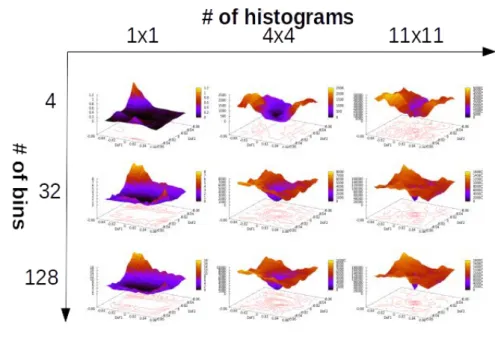
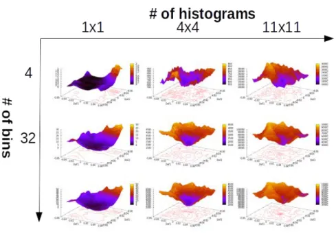
Using the methodology presented above, we compare empirically the cost functions generated by the following visual features: the raw intensity array (compared through the SSD, as perfor-mance baseline), the gray-levels histogram, the HS color histogram, the gray-levels histogram computed on an image synthesized from the H and S planes of a color image, and the His-togram of Oriented Gradients (HOG). First in nominal conditions, with fixed illumination and constant image quality, then with various perturbations. This will give us insights of how we can expect the features to perform in a robotic positioning task in a real environment (nomi-nal conditions give the best expected results, and perturbed conditions highlight the potential robustness to external changes in the environment). It will also help us determine the impact of the various parameters involved, such as the number of bins per histogram, as well as the

(49)

number of histograms per image.

It is important to note that the resulting cost function visualizations will be affected by the choice of the reference image’s appearance (performed here on a single test image). Hence, the analysis performed here is purely qualitative, in order to visualize potential trends in the cost function changes. This information will ease the parameter selection that will have to performed when setting up experiments in real scenes and leads to better performances.

3.2.3.2.1 Comparison of the methods in nominal conditions According to the following figures (Figs.3.8, 3.9, 3.10, 3.11, 3.12, corresponding to the cost function visualization as-sociated to, respectively, the SSD, the gray-levels histogram, the HS histogram and the HOG), we can see that the cost function shapes are greatly affected by the variation of the two param-eters (number of bins and number of histograms), and a trend can be observed: the increase in the number of bins tends to sharpen the cost function making it more precise around the global minimum (also increasing the computational complexity), and the increase in the num-ber of histograms tends to improve the convexity and sharpness, although in many cases, it also decreases the radius of the convex zone.

A resulting general rule for choosing an initial set of parameters is the following: for the number of bins, a noticeable improvement is seen by increasing it to at least 32, increasing it further yielding diminishing returns comparing to the increase in computational cost. For the number of histograms, choosing 4x4 histograms allows generally for a good trade-off between a large convex area and a good definition of the minimum, a lower number degrading the minimum noticeably, and a higher number reducing the convex area radius and increasing the computational cost. While comparing the 4 methods with each others, we can see that with a

-0.06 -0.04_-0.02 0 0.02 0.04 0.06-0.06-0.04 -0.02 0 0.02 0.04 0.06 0 1000 2000 3000 4000 5000 6000 7000 8000 9000 DoF1 DoF2 0 1000 2000 3000 4000 5000 6000 7000 8000 9000

Figure 3.8: SSD-based cost function