A General Framework for Computing Rearrangement Distances between Genomes with Duplicates

HAL Id: hal-00417735

https://hal.archives-ouvertes.fr/hal-00417735

Submitted on 16 Sep 2009

HAL is a multi-disciplinary open access

archive for the deposit and dissemination of sci-entific research documents, whether they are pub-lished or not. The documents may come from

L’archive ouverte pluridisciplinaire HAL, est destinée au dépôt et à la diffusion de documents scientifiques de niveau recherche, publiés ou non, émanant des établissements d’enseignement et de

A General Framework for Computing Rearrangement

Distances between Genomes with Duplicates

Sébastien Angibaud, Guillaume Fertin, Irena Rusu, Stéphane Vialette

To cite this version:

Sébastien Angibaud, Guillaume Fertin, Irena Rusu, Stéphane Vialette. A General Framework for Computing Rearrangement Distances between Genomes with Duplicates. Journal of Computational Biology, Mary Ann Liebert, 2007, 14 (4), pp.379-393. �10.1089/cmb.2007.A001�. �hal-00417735�

A Pseudo-Boolean Framework for Computing

Rearrangement Distances between Genomes with

Duplicates

S´ebastien Angibaud

Guillaume Fertin

Irena Rusu

St´ephane Vialette

22nd February 2007

Abstract

Computing genomic distances between whole genomes is a fundamental problem in comparative genomics. Recent researches have resulted in different genomic distance definitions: number of breakpoints, number of common intervals, number of conserved intervals, Maximum Adjacency Disruption number (MAD), etc. Unfortunately, it turns out that, in presence of duplications, most problems are NP-hard, and hence several heuristics have been recently proposed. However, while it is relatively easy to compare heuristics between them, until now very little is known about the absolute accuracy of these heuristics. Therefore, there is a great need for algorithmic approaches that compute exact solutions for these genomic distances. In this paper, we present a novel generic pseudo-boolean approach for computing the exact genomic distance between

∗_{Laboratoire d’Informatique de Nantes-Atlantique (LINA), FRE CNRS 2729 - Universit´e de Nantes, 2}

rue de la Houssini`ere, 44322 Nantes Cedex 3, France. E-mail: Sebastien.Angibaud@univ-nantes.fr

†_{Laboratoire d’Informatique de Nantes-Atlantique (LINA), FRE CNRS 2729 - Universit´e de Nantes, 2}

rue de la Houssini`ere, 44322 Nantes Cedex 3, France. E-mail: Guillaume.Fertin@univ-nantes.fr

‡_{Laboratoire d’Informatique de Nantes-Atlantique (LINA), FRE CNRS 2729 - Universit´e de Nantes, 2}

rue de la Houssini`ere, 44322 Nantes Cedex 3, France. E-mail: Irena.Rusu@univ-nantes.fr

§_{Laboratoire de Recherche en Informatique (LRI), UMR CNRS 8623 Facult´e des Sciences d’Orsay}

two whole genomes in presence of duplications, and put strong emphasis on common intervals under the maximum matching model. Of particular importance, we show three heuristics which provide very good results on a well-known public dataset of γ-Proteobacteria.

Keywords: pseudo-boolean programming, genome rearrangement, common inter-vals, duplication, heuristic.

1

Introduction

Due to the increasing amount of completely sequenced genomes, the comparison of gene

order is now becoming a standard approach in comparative genomics. A natural way to

compare species is to compare their whole genomes, where comparing two genomes is very

often realized by determining a measure of similarity (or dissimilarity) between them.

Sev-eral similarity (or dissimilarity) measures between two whole genomes have been proposed

and studied in the past few years, such as the number of breakpoints (Sankoff, 1999; Bryant,

2000; Blin et al., 2004; Goldstein et al., 2004; Chrobak et al., 2005), the number of

rever-sals (Bryant, 2000; El-Mabrouk, 2001; El-Mabrouk, 2002; Marron et al., 2004; Chen et al.,

2005; Swenson et al., 2005a; Swenson et al., 2005b; Fu et al., 2006; Kolman and Wale´n, 2006;

Kolman and Wale´n, 2007), the number of conserved intervals (Blin and Rizzi, 2005; Chen

et al., 2006a), the number of common intervals (Bourque et al., 2005), the Maximum

Adja-cency Disruption Number (MAD) (Sankoff and Haque, 2005), etc. However, in the presence

of duplications and for each of the above measures, one has first to disambiguate the data by

Up to now, two extremal approaches have been considered: the exemplar matching model

and the maximum matching model. In the exemplar matching model (Sankoff, 1999), for

all duplicated genes, all but one occurrence in each genome are deleted. In the maximum

matching model (Blin et al., 2004; Goldstein et al., 2004; Chrobak et al., 2005; Chen et al.,

2005; Fu et al., 2006; Chauve et al., 2006; Kolman and Wale´n, 2007), the goal is to map as

many genes as possible. These two models can be considered as the extremal cases of the

same generic homolog assignment approach.

Unfortunately, it has been shown that, for each of the above mentioned measures,

what-ever the considered model (exemplar or maximum matching), the problem becomes NP-hard

as soon as duplicates are present in genomes (Bryant, 2000; Blin et al., 2004; Blin and Rizzi,

2005; Chauve et al., 2006) ; some inapproximability results are known for some special

cases (Thach, 2005; Chen et al., 2006b; Chen et al., 2006a). Therefore, several heuristic

methods have been recently devised to obtain (hopefully) good solutions in a reasonable

amount of time (Blin et al., 2005; Bourque et al., 2005). However, while it is relatively

easy to compare heuristics between them, until now very little is known about the absolute

accuracy of these heuristics. Therefore, there is a great need for algorithmic approaches that

compute exact solutions for these genomic distances.

In the present paper, we introduce a novel generic pseudo-boolean programming approach

for computing exact solutions. In this first attempt, we focus on the problem of finding the

maximum number of common intervals between two genomes under the maximum matching

model. From a computational point of view, the problem of computing a matching that

maximizes the number of common intervals (together with MAD) is one of the hardest in

the main idea of our approach: a pseudo-boolean program together with reduction rules.

We also present three heuristics for solving this problem, and we compare their results to

the ones obtained by the pseudo-boolean program on a dataset of γ-Proteobacteria.

This paper is organized as follows. In Section 2, we present some preliminaries and

definitions. We focus in Section 3 on the problem of finding the maximum number of common

intervals under the maximum matching model, and give a pseudo-boolean programming

approach together with some reduction rules. Section 4 is devoted to experimental results

on a dataset of γ-Proteobacteria. In particular, in this section we define three different

heuristics and we prove that they provide very good results on our dataset.

2

Preliminaries

Genomes with duplications are usually represented by signed sequences over the alphabet

of gene families, where every element in a genome is a gene. However, in order to simplify

notations, and since common intervals do not depend on the sign given to the genes, we will

consider only unsigned genomes in the rest of the paper. Any gene belongs to a gene family,

and two genes belong to the same gene family if they have the same label. In the sequel,

we will be extensively concerned with pairs of genomes. Let G1 and G2 be two genomes,

and let a ∈ {1, 2}. The number of genes in genome Ga is always written na. We denote

the i-th gene of genome Ga by Ga[i]. For any 1 ≤ i ≤ j ≤ na, we write Ga(i, j) for the set

{Ga[i], Ga[i+1], . . . , Ga[j]} and we let Gastand for Ga(1, na). In other words, Ga(i, j) is the set

of all distinct genes between positions i and j in genome Ga, while Ga is the set of all distinct

genes in the whole genome Ga. For any gene g ∈ Ga and any 1 ≤ i ≤ j ≤ na, we denote by

To simplify notations, we abbreviate occa(g, 1, na) to occa(g).

A matching M between genomes G1and G2 is a set of pairwise disjoint pairs (G1[i], G2[j]),

where G1[i] and G2[j] belong to the same gene family, i.e., G1[i] = G2[j]. Genes of G1 and

G2 that do not belong to any pair of the matching M are said to be unmatched for M. A

matching M between G1 and G2 is said to be maximum if for any gene family f , there are

no two genes of f that are unmatched for M and belong to G1 and G2, respectively. A

matching M between G1 and G2 is said to be exemplar if for any gene family f , exactly one

gene of f is matched by M between G1 and G2. A matching M between G1 and G2 can

be seen as a way to describe a putative assignment of orthologous pairs of genes between

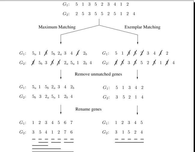
G1 and G2 (see for example (Chen et al., 2005) ; see also Figure 1 for an illustration of the

exemplar and maximum matching concepts).

Let M be any matching between G1 and G2. By first deleting unmatched genes and next

renaming genes in G1 and G2 according to the matching M, we may now assume that both

G1 and G2 are duplication-free, i.e., G2 is a permutation of G1.

It is easily seen that, by first resorting to a renaming procedure, we can always assume

that one of the two genomes, say G1, is the identity permutation, i.e., G1 = 1 2 . . . n1 (an

illustration is shown in the bottom part of Figure 1).

A common interval between G1and G2is a substring of G1, i.e., a sequence of consecutive

genes of G1, for which the exact same content can be found in a substring of G2 (see for

instance (Uno and Yagiura, 2000; Landau et al., 2005; Bergeron et al., 2005)). For example,

let G1 = 1 2 3 4 5 and G2 = 1 5 3 4 2. Then, the interval [3 : 5] of G1 is a common

interval (because 5 3 4 occurs as a substring in G2). Notice that there exists at least n + 1

a common interval and G1 itself is also a common interval. This lower bound is tight as

shown by G1 = 1 2 3 4 and G2 = 2 4 1 3. Furthermore, if G1 = G2 the number of common

intervals between G1 and G2 is n(n+1)₂ , where n = n1 = n2, i.e., each possible substring of

G1 is a common interval.

-Figure 1 should go

here-3

An exact algorithm for maximizing the number of

common intervals

In this section, we are interested in the following problem: given two genomes that contain

duplicates, find a maximum matching that maximizes the number of common intervals.

We show how this problem can be transformed into an equivalent pseudo-boolean problem.

The section is organized as follows: in Section 3.1, we briefly introduce basic and general

notions concerning pseudo-boolean programs. Section 3.2 shows how to transform our initial

problem into a pseudo-boolean program, while Section 3.3 shows how this program can be

simply modified in order to compute the maximum number of common intervals between

two genomes under two other models: the exemplar matching model and the intermediate

model, where at least one gene in each gene family is mapped. Finally, Section 3.4 contains

a set of rules which will help speed-up the program by avoiding the generation of a large

3.1

Pseudo-boolean models

A Linear Pseudo-boolean (LPB) program is a linear program (Schrijver, 1998) where all

variables are restricted to take values of either 0 or 1. For one, LPB programs are viewed by

the linear programming community as just a domain restriction on general linear

program-ming. For another, from a satisfiability (Sat) point of view, pseudo-boolean constraints can

be seen as a generalization of clauses providing a significant extension of purely propositional

constraints (Chai and Kuehlmann, 2003; E´en and S¨orensson., 2006).

Conventionally, LPB problems are handled by generic Integer Linear Programming (ILP)

solvers. The drawback of such an approach is that generic ILP solvers typically ignore the

boolean nature of the variables. Alternatively, LPB decision problems could be encoded as

Sat _{instances in pure CNF (Conjunctive Normal Form), i.e., conjunction of disjunctions}

of boolean literals, which are then solved by any of the highly specialized Sat approaches.

However the number of clauses required for expressing the LPB constraints is prohibitively

large. Moreover a pure CNF encoding may prevent the solver from pruning the search space

efficiently (Chai and Kuehlmann, 2003). Boolean satisfiability solvers available today are the

result of decades of research and are deemed to be among the faster NP-hard problem specific

solvers. The latest generation of Sat solvers generally have three key features (randomization

of variable selection, backtracking search and some form of clause learning) and they usually

run in reasonable time (even for very large instances).

A number of generalizations of Sat solvers to LPB solvers have been proposed (Pueblo (Sheini

and Sakallah, 2006), Galena (Chai and Kuehlmann, 2003), OPBDP (Barth, 2005) and more).

We decided to use for our tests the minisat+ LPB solver (E´en and S¨orensson., 2006) because

3.2

Common intervals in the Maximum Matching Model

We propose in Figure 2 a pseudo-boolean program for computing the maximum number of

common intervals between two genomes under the maximum matching model in the presence

of duplications (we assume here that each gene g ∈ G1 ∪ G2 occurs both in G1 and in G2 ;

if this is not the case, a pre-process of G1 and G2 will delete from G1 and G2 those genes

which appear in only one genome).

-Figure 2 should go

here-Program Common-Intervals-Matching is clearly a pseudo-boolean program, i.e., a (0,

1)-linear program. Roughly speaking, the boolean variables are divided in two sets: true setting

of variables in C denote possible common intervals between G1 and G2, while true setting

of variables in X denote the mapping, i.e., matching, between G1 and G2.

We now turn to describing the constraints. Constraints in (C.01) and in (C.02) deal

with consistency of the mapping: each gene of G1 is mapped to at most one gene of G2, and

conversely (some genes need indeed to be deleted in case of unbalanced families).

Constraints in (C.03) ensure that each common interval is counted exactly once. The

key idea here is to impose an “active border” property, i.e., if variable ci,j_k,` is set to 1 then

genes G1[i] and G1[j] must match some distinct genes between positions k and ` in G2, and

genes G2[k] and G2[`] must match some distinct genes between positions i and j in G1. More

intuitively, this constraint ensures that a common interval will not be counted more than

once, by forcing each extremity of a common interval to be matched.

Constraints in (C.04) to (C.07) ensure that if ci,j_k,` = 1 then the interval [i : j] of G1 and

true setting of X. For example, constraints in (C.04) ensure that each gene in the interval

[i : j] of G1 is either not mapped or is mapped to a gene in the interval [k : `] of G2 (thanks

to constraints in (C.01), (C.02) and (C.03), genes at position i and j in G1 are actually

mapped to distinct genes in G2 if i < j and ci,jk,` = 1).

Finally, constraints in (C.08) force the mapping to be a maximum matching between G1

and G2.

Proposition 1. Program Common-Intervals-Matching correctly computes the maximum

number of common intervals between G1 and G2 under the maximum matching model.

We briefly discuss here space issues of Program Common-Intervals-Matching. First,

it is easily seen that #C = Θ(n2

1n22) and hence that (C.03) is composed of Θ(n21n22)

con-straints. The number of constraints in (C.04) to (C.07) however does depend on the number

of duplications in the two genomes. Second, #X = O(n1n2). Clearly, the size of the set X

determines the number of constraints in (C.01) and (C.02) and of course strongly depends

on the number of duplications in G1 and G2. Not surprisingly, set X turns out to be of

mod-erate size in practice. Finally, the number of constraints in (C.08) is clearly linear in the

size of the two genomes. We shall soon describe (section 3.4) how to speed-up the program

by reducing the number of variables and constraints. Before that, we show in the

follow-ing section how to modify the Program Common-Intervals-Matchfollow-ing in order to compute

the maximum number of common intervals between two genomes under, respectively, the

exemplar matching model and the intermediate model, where at least one gene in each gene

3.3

Adapting the Program for other Models

In this section, we point out the genericity of the pseudo-boolean framework for computing

a matching that maximizes the number of common intervals between two genomes. Indeed,

we show here a fast and easy way to modify the Program Common-Intervals-Matching in

order to compute the maximum number of common intervals between two genomes under

two other models: the exemplar matching model and the intermediate model, where at least

one gene in each gene family is mapped.

We observe indeed that replacing constraints in (C.08) by a new set of constraints (C.08’)

– see below – in Program Common-Intervals-Matching results in the pseudo-boolean

pro-gram Common-Intervals-Exemplar that computes the maximum number of common

inter-vals between genomes G1 and G2 under the exemplar matching model.

(C.08’) ∀g ∈ G1∪ G2, P 1≤i≤n1 G1[i]=g P 1≤k≤n2 G2[k]=g xi_k= 1

Interestingly enough, substituting now the constraints in (C.08) by a new set of

con-straints (C.08’’) – see below – in Program Common-Intervals-Matching results in a

pseudo-boolean program that computes the maximum number of common intervals between genomes

G1 and G2 under the following intermediate model: at least one gene in each gene family

is mapped. Observe that this model contains both the exemplar matching model and the

maximum matching model as special cases.

(C.08’’) ∀g ∈ G1∪ G2, P 1≤i≤n1 G1[i]=g P 1≤k≤n2 G2[k]=g xi_k≥ 1

3.4

Speeding-up the program

We give in this section four rules for speeding-up Program Common-Intervals-Matching.

In theory, a very large instance may be easy to solve and a small instance hard. However,

very often, small hard instances turn out be artificial, e.g., the pigeonhole problem, and

hence, in case of practical instances, the running time of a pseudo-boolean solver is most

of the time related to the size of the instances. The main idea here is thus to reduce the

number of variables and constraints in the program (for ease of exposition, we describe our

rules as filters on C). More precisely, we give rules that avoid introducing useless variables

ci,j_k,` in C in such a way that the correctness of Program Common-Intervals-Matching is

maintained by repeated applications of the rules ; two of these filters however do modify the

correct maximum number of common intervals between the two genomes and thus ask for

subsequent modifications in order to obtain the correct solution.

[Rule 1] Delete from C all variables ci,i_k,k, 1 ≤ i ≤ n1 and 1 ≤ k ≤ n2.

Rule 1 does modify the correct number of common intervals between G1 and G2, and

hence application of this rule asks for subsequent modifications of the number of common

intervals. The key idea of Rule 1 is simply to discard common intervals of size 1 from the

program. Indeed, we can compute in a pre-processing step the numbers d1 and d2 of genes

that need to be deleted in G1 and G2 for obtaining a maximum matching between the two

genomes. Therefore, we know that the resulting genomes will consist in L = n1−d1 = n2−d2

genes, where

L=X

g∈G

But each of these genes will contribute for 1 to the number of common intervals between G1

and G2, for any maximum matching. We thus simply delete all these variables and add L to

the number of common intervals between G1and G2found by Program Common-Intervals-Matching.

[Rule 2] Delete from C all variables ci,j_k,` for which any of the following conditions holds true:

1. (#{r : k ≤ r ≤ ` ∧ G1[i] = G2[r]} = 0) ∨ (#{s : k ≤ s ≤ ` ∧ G1[j] = G2[s]} = 0),

2. (#{r : k ≤ r ≤ ` ∧ G1[i] = G2[r]} < 2) ∧ (G1[i] = G1[j]),

3. (#{p : i ≤ p ≤ j ∧ G2[k] = G1[p]} = 0) ∨ (#{q : i ≤ q ≤ j ∧ G2[`] = G1[q]} = 0),

4. (#{p : i ≤ p ≤ j ∧ G2[k] = G1[p]} < 2) ∧ (G2[k] = G2[`]).

Rule 2 is a quickening for constraints in (C.03). Indeed, these constraints ensure that

each common interval is counted exactly once by the program by forcing the border of each

common interval to be active in the computed solution, i.e., genes G1[i] and G1[j] match

some distinct genes between positions k and ` in G2, and genes G2[k] and G2[`] match some

distinct genes between positions i and j in G1. Correctness of Rule 2 thus follows from the

fact that Program Common-Intervals-Matching will always set a variable ci,j_k,` to 0 if the

border property cannot be satisfied (it is assumed here that i < j and k < `).

[Rule 3] Delete from C all variables ci,j<sub>k,`</sub> for which there exists at least one gene g ∈ G such that |occ1(g, i, j) − occ2(g, k, `)| > |occ1(g) − occ2(g)|.

Roughly speaking, Rule 3 avoids us to delete too many genes in a common interval.

Indeed, for one, for any g ∈ G, |occ1(g, i, j) − occ2(g, k, `)| is clearly the minimum number

of occurrences of gene g that need to be deleted if ci,j<sub>k,`</sub> = 1, i.e., [i : j] and [k : `] form a

common interval between the two genomes. For another, for any g ∈ G, |occ1(g) − occ2(g)|

is the number of occurrences of gene g that need to be deleted in G1 and G2 for finding any

maximum matching between the two genomes. Correctness of Rule 3 thus follows from the

[Rule 4] Delete from C all variables ci,j_k,` for which the four following conditions hold true: 1. ∀g ∈ G1(i, j), #occ1(g, 1, i − 1) + #occ1(g, j + 1, n1) = 0,

2. ∀g ∈ G2(k, `), #occ2(g, 1, k − 1) + #occ2(g, ` + 1, n2) = 0,

3. #occ1(G1[i]) ≤ #occ2(G1[i]) ∧ #occ1(G1[j]) ≤ #occ2(G1[j]),

4. #occ2(G2[k]) ≤ #occ1(G2[k]) ∧ #occ2(G2[`]) ≤ #occ1(G2[`]).

We first observe that Rule 4 does modify the correct number of common intervals

between G1 and G2, and hence application of this rule asks for subsequent modifications

of the number of common intervals. The rationale of Rule 4 is that, if the four conditions

hold true, then ci,jk,` will always be set to 1 by Program Common-Intervals-Matching. In

other words, for any maximum matching between G1 and G2, [i : j] and [k : `] will form a

common intervals. We thus simply delete from C all these variables ci,j_k,` and add the number

of deleted variables by Rule 4 to the number of common intervals between G1 and G2 found

by Program Common-Intervals-Matching. This rule will prove extremely useful for highly

conserved regions with localized duplications.

4

Experimental results

As mentioned in the Introduction, the generic pseudo-boolean approach we propose in this

paper can be useful for estimating the accuracy of one or several heuristic(s). In that

perspective, it is necessary to compute the exact results for different datasets, that could

be later used as benchmarks to which confront the results given by any given heuristic

algorithm. In this section, we will compare the exact results we have obtained from a given

dataset by our pseudo-boolean method to three heuristics, respectively called ILCS, IILCS

The three heuristics we will study in the following are:

• the heuristic ILCS, which is a small variant of the one used in (Blin et al., 2005)

• an improvement we suggest for ILCS (that we will denote IILCS)

• a hybrid method, called HYBk, that mixes the approach used in the IILCS heuristic

and the pseudo-boolean approach. We will mainly be interested in the case where

parameter k is equal to 2.

We will thus compare the results obtained by the ILCS, IILCS and HYB2 heuristics to

the exact results we have obtained via our pseudo-boolean approach. In particular, we will

show that IILCS and HYB2 perform very well on the dataset we used. Before that, we first

describe this dataset, and we present each of the three above mentioned heuristics in details.

4.1

Exact Results

We performed the computation of exact results concerning common intervals in the maximum

matching model by studying the dataset used in (Blin et al., 2005). This dataset is composed

of 12 complete genomes from the 13 γ-Proteobacteria originally studied in (Lerat et al.,

2003). The thirteenth genome (V.cholerae) was not considered, since it is composed of

two chromosomes, and hence does not fit in the model we considered here for representing

genomes. More precisely, this dataset is composed of the genomes of the following species:

• Buchnera aphidicola APS (Baphi, Genbank accession number NC 002528),

• Escherichia coli K12 (Ecoli, NC 000913),

• Pseudomonas aeruginosa PA01 (Paeru, NC 002516),

• Pasteurella multocida Pm70 (Pmult, NC 002663),

• Salmonella typhimurium LT2 (Salty, NC 003197),

• Xanthomonas axonopodis pv. citri 306 (Xaxon, NC 003919),

• Xanthomonas campestris (Xcamp, NC 0 03902),

• Xylella fastidiosa 9a5c (Xfast, NC 002488),

• Yersinia pestis CO 92 (Ypest-CO92, NC 003143),

• Yersinia pestis KIM5 P12 (Ypest-KIM, NC 004088) and

• Wigglesworthia glossinidia brevipalpis Baphi (NC 004344).

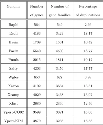
The computation of a partition of the complete set of genes into gene families, where each

family is supposed to represent a group of homologous genes, is taken from (Blin et al., 2005)

(this partition was actually provided to these authors by Lerat (Lerat et al., 2003)). The

main characteristics (number of genes, number of gene families, percentage of duplicates) of

the twelve considered genomes are summarized in Table 1.

-Table 1 should go

here-Despite the fact that the model (maximum matching model) and the measure (number

of common intervals) we study are one of the most time consuming, nearly two thirds of the

exact results have been computed until now. It is also interesting to note that, for three

Wigglesworthia glossinidia brevipalpis), we have obtained all the exact results that involve

those genomes.

These results, though still partial, allow us to go further ; indeed, thanks to the exact

results we have obtained, we are now able to confront the results given by three different

heuristics to them. Those three heuristics are now presented in details.

4.2

The ILCS Heuristic

We first start by describing the heuristic that we will call ILCS (Iterative Longest Common

Substring). It is actually a small variant of the one used in (Blin et al., 2005). This heuristic

is greedy, and works as follows:

1. Compute the Longest Common Substring (i.e., the longest contiguous word) S of the

two genomes, up to a complete reversal. If there are several candidates, pick one at

random

2. Match all the genes of S accordingly

3. Iterate the process until all possible genes have been matched (i.e., we have obtained

a maximum matching)

4. Remove, in each genome, all the genes that have not been matched

5. Compute the number of common intervals that have been obtained in this solution

For instance, suppose that G1 = 1 2 3 4 5 6 7 and G2 = 6 7 4 5 1 6 3 2 1. Below is a

brief description of the running of ILCS, where the parts which are underlined represent the

1 2 3 4 5 6 7 6 7 4 5 1 6 3 2 1 1 2 34 5 6 7 6 7 4 5 1 6 3 2 1 1 2 3 4 56 7 6 7 4 5 1 6 3 2 1 1 2 3 4 5 6 7 6 7 4 5 3 2 1

In this example, the number of Common Intervals we obtain is equal to 19.

The simple idea behind this heuristic algorithm is that a Longest Common Substring (up

to complete reversal) of length k contains k(k+1)₂ common intervals. Hence, finding such exact

copies in both genomes intuitively helps to increase the total number of common intervals.

4.3

The IILCS Heuristic: an improvement of ILCS

A closer look on the ILCS heuristic led us to suggest an improvement to it, in the form

of a new heuristic, that we call IILCS (Improved Iterative Longest Common Substring).

Heuristic IILCS works as follows:

1. Compute the Longest Common Substring S of the two genomes, up to a complete

reversal. If there are several candidates, pick one at random

2. Match all the genes of S accordingly

3. Remove from genome G1 (resp. G2) the unmatched gene(s) for which there remains

no unmatched genes of the same family in G2 (resp. G1)

4. Iterate the process until all possible genes have been matched (i.e., we have obtained

5. Compute the number of common intervals that have been obtained in this solution

The only difference between IILCS and ILCS lies in line 3: intuitively, before searching

for a Longest Common Substring (up to a complete reversal), we “tidy” the two genomes.

More precisely, we remove, in each genome and at each iteration, the genes for which we

know they will not be matched in the final solution ; such genes are unmatched genes for

which there remains no “corresponding” (i.e., of the same family) unmatched gene in the

other genome. This process can simply be undertaken by counting, at each iteration, the

number of unmatched genes of each gene family in both genomes. This actually allows to

find Longest Common Substrings that are possibly longer than the ones found in the ILCS

heuristic.

For example, let us take the same instance as the one used in the previous section, that

is G1 = 1 2 3 4 5 6 7 and G2 = 6 7 4 5 1 6 3 2 1. Below is a brief description of the running

of IILCS, where the parts which are underlined represent the Longest Common Substring,

genes in italic are genes that are going to be removed (because they have no unmatched gene

of the same family in the other genome), and genes in bold are matched.

1 2 3 4 5 6 7 6 7 4 5 1 6 3 2 1 1 2 34 5 6 7 6 7 4 5 6 3 2 1 1 2 34 5 6 7 6 7 4 5 6 3 2 1 1 2 3 4 5 67 7 4 5 6 3 2 1 1 2 3 4 5 67 7 4 5 6 3 2 1 1 2 3 4 5 6 7 6 7 4 5 3 2 1

In this example, the number of Common Intervals we obtain is equal to 20.

4.4

The Hybrid Method HYB

Starting from the IILCS heuristic, one can think of a further improvement: first, use the

IILCS method until no Longest Common Substring of size greater than or equal to k exists

(where k is a given parameter) ; this will give a partially solved instance, in the sense that

some genes are matched while some are not. Second, in order to totally solve the problem,

we run our pseudo-boolean program on the partially solved instance.

The HYBk method can be described as follows:

1. Run the IILCS method until no Longest Common Substring of size greater than or

equal to k exists

2. Give the partially solved instance obtained above as an input to the pseudo-boolean

program Common-Intervals-Matching

3. Compute the number of common intervals that have been obtained in this solution

Since the pseudo-boolean program will always output the best (i.e., exact) result, and

since before calling the pseudo-boolean program we run the IILCS heuristic, we can ensure

that HYBk is at least as good as IILCS for any value of k and any given instance (G1, G2).

However, the main drawback of HYBk compared to IILCS concerns the running time ;

indeed, IILCS is a polynomial time algorithm, while there is no guarantee that HYBk (for

any k ≥ 2) will ever answer, even on a very powerful computer. This is because we are

asking for an exact result in the second part of the algorithm, which means that it runs in

be matched by the IILCS part of the heuristic, and one can hope for the exact result to

be computed relatively fast. Moreover, the exact part of the HYBk heuristic is run through

our pseudo-boolean program, which has been designed to speed-up the computation. In

that sense, HYBk appears as a compromise between the exactness of the results and the

computation time.

For our experiments, we will choose the smallest possible value for k, that is k = 2.

The results we have obtained through our HYBk method are at the same time promising

and somehow disappointing ; they are promising in terms of quality of the results (more

details are provided in Section 4.5), but disappointing in terms of running time. Indeed,

even when fixing k as small as possible (that is, k = 2), only 46 out of the 66 possible

pairwise comparisons were obtained within a few days of computation, that is, only 6 more

results than the exact method.

4.5

Results and Discussion

Out of the 66 possible pairwise genome comparisons, 40 results have been obtained within

a few days of computation. More precisely, among these 40 values, only 4 of them took

several days to be computed (Haein/Pmult, Haein/Xfast, Paeru/Pmult and Paeru/Xfast),

while the others took no more than a few minutes.

One of the main interests of our pseudo-boolean approach is that the exact results they

provide can be used to test the robustness of some heuristic(s). We have thus confronted

the 40 exact results we have obtained to the results given by the three heuristics we have

presented in the previous sections.

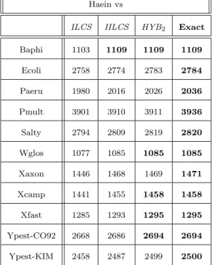
for Buchnera aphidicola are summarized in Table 2, results for Haemophilus influenzae are

summarized in Table 3, while results concerning Wigglesworthia glossinidia brevipalpis are

summarized in Table 4.

Looking at these results, we can see that, non surprisingly, HYB2 is always better or as good

as IILCS, which is itself always better or as good as ILCS. In particular, HYB2 returns the

optimal value in all the cases for Buchnera aphidicola, in 5 out of the 11 cases for Haemophilus

influenzae, and in 9 out of the 11 cases for Wigglesworthia glossinidia brevipalpis.

-Table 2 should go

-Table 3 should go

-Table 4 should go

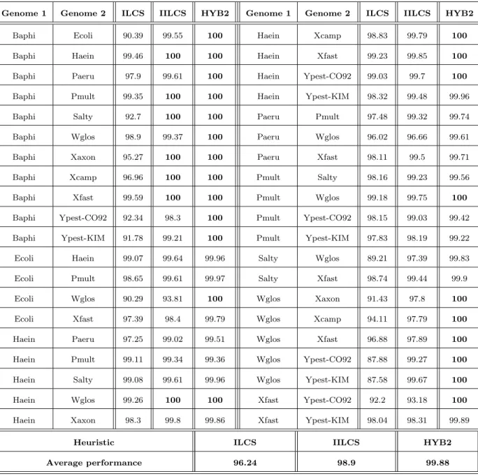
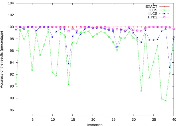
here-A more global view at the respective performances of heuristics ILCS, IILCS and HYB2

is given in Table 5. In this table, for each of the 40 exact results we have obtained, and

for each heuristic H, we provide the ratio _ICIC_{(OP T )}(H) , where IC(H) is the number of common

intervals returned by H and IC(OP T ) is the exact number of common intervals. This

ra-tio is given as a percentage. These results are also illustrated in a graphical form in Figure 3.

These results confirm that HYB2 is always better (or as good as) IILCS, which is always

better (or as good as) ILCS: more precisely, on average, IILCS improves by 2.66% the

per-formances of ILCS, while HYB2 improves by a further 0.98% the performances of IILCS.

good on the dataset we studied. Indeed, out of the 40 instances for which we have

com-puted the exact results, IILCS returns the optimal result in 7 cases, and returns a number

of common intervals that is more than 99% of the optimal number for 22 other cases. The

“worse” result that IILCS provides is 93.18% away from the optimal (Xfast/Ypest-CO92).

On average, over the 40 pairwise comparisons for which we have exact results, IILCS gives

a number of common intervals that is 98.9% of the optimal number.

Concerning heuristic HYB2, out of the 40 instances for which we have computed the exact

results, it returns the optimal result in 23 cases, and returns a number of common intervals

that is more than 99% of the optimal number for the remaining 17 other cases. The “worse”

result that HYB2 provides is 99.22% away from the optimal (Pmult/Ypest-KIM). On

aver-age, over the 40 pairwise comparisons for which we have exact results, HYB2 gives a number

of common intervals that is 99.88% of the optimal number.

-Table 5 should go

-Figure 3 should go

here-These results come as a surprise, because, despite being extremely simple and fast, IILCS

appears to be extremely good on this dataset. HYB2 works even better on this dataset, but

its main drawback is that we have no guarantee on its execution time. Hence, this strongly

suggests that computing common intervals in the maximum matching model can simply be

undertaken using either IILCS or HYB2 (depending on the execution time of HYB2), while

5

Conclusion

In this paper, we have introduced a novel and original method that helps speeding-up

com-putations of exact results for comparing whole genomes containing duplicates. This method

makes use of pseudo-boolean programming. Our approach is very general, and can handle

several (dis)similarity measures (breakpoints, common intervals, conserved intervals, MAD,

etc.) under several possible models (exemplar matching model, maximum matching model,

but also most models within those two extrema).

An example of such an approach (common intervals under the maximum matching model)

has been developed, in order to illustrate the main ideas of the pseudo-boolean

transforma-tion framework that we suggest. Experiments have also been undertaken on a dataset of

γ-Proteobacteria, showing the validity of our approach, since 40 results (out of 66) have been

obtained in a limited amount of time. Moreover, these preliminary results have allowed us to

state that, in particular, both the IILCS and the HYB2 heuristics provide excellent results

on this dataset, hence showing their validity and robustness (though there is no guarantee on

the execution time of HYB2). On the whole, these preliminary results are very encouraging.

Our approach is in fact more ambitious. Our long term goal is indeed to develop a generic

pseudo-boolean approach for the exact computation of various genome distances (number of

breakpoints, number of common intervals, number of conserved intervals, MAD, etc.) under

both the exemplar and the maximum matching models, and use this generic approach on

different datasets. The rationale of this approach is threefold:

1. There is a crucial need for new algorithmic solutions providing exact genome distances

the accuracy of existing heuristics and to design new efficient biologically relevant

heuristics.

2. Very little is known about the relations between the various genome distances that

have been defined so far (number of breakpoints, number of common intervals, number

of conserved intervals, MAD, etc.). We thus propose to extensively compare all these

genome distances under both models with a generic pseudo-boolean framework on

several datasets.

3. We also plan to further investigate the relations between the exemplar and the

max-imum matching models. We strongly believe here that, in the light of these

compar-isons, some biologically relevant intermediate model between these two extrema could

be defined.

There is still a great amount of work to be done, and some of it is being undertaken by

the authors at the moment. Among other things, one can cite:

• Implementing and testing all the possible above mentioned models, for all the possible

above mentioned (dis)similarity measures,

• For each case, determining strong and relevant rules for speeding-up the process by

avoiding the generation of a large number clauses and variables (a pre-processing step

that should not be underestimated),

• Obtaining exact results for each of these models and measures, and for different

datasets, that could be later used as benchmarks in order to validate (or not)

References

Barth, P. (2005). A Davis-Putnam based enumeration algorithm for linear pseudo-Boolean

optimization. Technical Report MPI-I-95-2-003, Max Planck Institut Informatik. 13

pages.

Bergeron, A., Chauve, C., de Montgolfier, F., and Raffinot, M. (2005). Computing common

intervals of K permutations, with applications to modular decomposition of graphs. In

Proc. 5th Workshop on Algorithms in Bioinformatics (WABI), volume 3669 of LNCS,

pages 779–790.

Blin, G., Chauve, C., and Fertin, G. (2004). The breakpoint distance for signed sequences.

In Proc. 1st Algorithms and Computational Methods for Biochemical and Evolutionary

Networks (CompBioNets), pages 3–16. KCL publications.

Blin, G., Chauve, C., and Fertin, G. (2005). Genes order and phylogenetic

reconstruc-tion: Application to γ-proteobacteria. In Proc. 3rd RECOMB Comparative Genomics

Satellite Workshop, volume 3678 of LNBI, pages 11–20.

Blin, G. and Rizzi, R. (2005). Conserved intervals distance computation between

non-trivial genomes. In Proc. 11th Annual Int. Conference on Computing and

Combina-torics (COCOON), volume 3595 of LNCS, pages 22–31.

Bourque, G., Yacef, Y., and El-Mabrouk, N. (2005). Maximizing synteny blocks to identify

ancestral homologs. In Proc. 3rd RECOMB Comparative Genomics Satellite Workshop,

volume 3678 of LNBI, pages 21–35.

Bryant, D. (2000). The complexity of calculating exemplar distances. In Comparative

Align-ment, and the Evolution of Gene Families, pages 207–212. Kluwer.

Chai, D. and Kuehlmann, A. (2003). A fast pseudo-boolean constraint solver. In Proc.

40th ACM IEEE conference on Design automation, pages 830–835.

Chauve, C., Fertin, G., Rizzi, R., and Vialette, S. (2006). Genomes containing

dupli-cates are hard to compare. In Proc Int. Workshop on Bioinformatics Research and

Applications (IWBRA), volume 3992 of LNCS, pages 783–790.

Chen, X., Zheng, J., Fu, Z., Nan, P., Zhong, Y., Lonardi, S., and Jiang, T. (2005).

Assignment of orthologous genes via genome rearrangement. IEEE/ACM Transactions

on Computational Biology and Bioinformatics, 2(4):302–315.

Chen, Z., Fowler, R., Fu, B., and Zhu, B. (2006a). Lower bounds on the approximation

of the exemplar conserved interval distance problem of genomes. In Proc. 12th Annual

International Computing and Combinatorics Conference (COCOON’06), volume 4112

of LNCS, pages 245–254.

Chen, Z., Fu, B., and Zhu, B. (2006b). The approximability of the exemplar breakpoint

distance problem. In Proc. 2nd International Conference on Algorithmic Aspects in

Information and Management (AAIM’06), volume 3328 of LNCS, pages 291–302.

Chrobak, M., Kolman, P., and Sgall, J. (2005). The greedy algorithm for the minimum

common string partition problem. ACM Transactions on Algorithms, 1(2):350–366.

E´en, N. and S¨orensson., N. (2006). Translating pseudo-boolean constraints into SAT.

Journal on Satisfiability, Boolean Modeling and Computation, 2:1–26.

El-Mabrouk, N. (2001). Sorting signed permutations by reversals and insertions/deletions

El-Mabrouk, N. (2002). Reconstructing an ancestral genome using minimum segments

duplications and reversals. Journal of Computer and System Sciences, 65:442–464.

Fu, Z., Chen, X., Vacic, V., Nan, P., Zhong, Y., and Jiang, T. (2006). A parsimony

approach to genome-wide ortholog assignment. In Proc. 10th Annual International

Conference on Research in Computational Molecular Biology (RECOMB), volume 3909

of LNBI, pages 578–594.

Goldstein, A., Kolman, P., and Zheng, J. (2004). Minimum common string partition

problem: Hardness and approximations. In Proc. 15th International Symposium on

Algorithms and Computation (ISAAC), volume 3341 of LNCS, pages 484–495.

Kolman, P. and Wale´n, T. (2006). Reversal distance for strings with duplicates: Linear

time approximation using hitting set. In Proc. 4th Workshop on Approximation and

Online Algorithms (WAOA), volume 4368 of LNCS, pages 281–291.

Kolman, P. and Wale´n, T. (2007). Approximating reversal distance for strings with

bounded number of duplicates. Discrete Applied Mathematics, 155(3):327–336.

Landau, G., Parida, L., and Weimann, O. (2005). Gene proximity analysis across whole

genomes via PQ trees. Journal of Computational Biology, 12(10):1289–1306.

Lerat, E., Daubin, V., and Moran, N. (2003). From gene tree to organismal phylogeny in

prokaryotes: the case of γ-proteobacteria. PLoS Biology, 1(1):101–109.

Marron, M., Swenson, K., and Moret, B. (2004). Genomic distances under deletions and

insertions. Theoretical Computer Science, 325(3):347–360.

Sankoff, D. (1999). Genome rearrangement with gene families. Bioinformatics, 15(11):909–

Sankoff, D. and Haque, L. (2005). Power boosts for cluster tests. In Proc. 3rd RECOMB

Comparative Genomics Satellite Workshop, volume 3678 of LNBI, pages 11–20.

Schrijver, A. (1998). Theory of Linear and Integer Programming. John Wiley and Sons.

Sheini, H. and Sakallah, K. (2006). Pueblo: A hybrid pseudo-boolean SAT solver. Journal

on Satisfiability, Boolean Modeling and Computation, 2:165–189.

Swenson, K., Marron, M., Earnest-DeYoung, J., and Moret, B. (2005a). Approximating

the true evolutionary distance between two genomes. In Proc. 7th Workshop on

Algo-rithms Engineering and Experiments and Second Workshop on Analytic Algorithmics

and Combinatorics (ALENEX, SIAM Press, pages 121–129.

Swenson, K., Pattengale, N., and Moret, B. (2005b). A framework for orthology

assign-ment from gene rearrangeassign-ment data. In Proc. 3rd RECOMB Workshop on Comparative

Genomics (RECOMB-CG), volume 3678 of LNBI, pages 153–166.

Thach, N. C. (2005). Algorithms for calculating exemplar distances. Honours Year Project

Report, National University of Singapore.

Uno, T. and Yagiura, M. (2000). Fast algorithms to enumerate all common intervals of

Maximum Matching

Remove unmatched genes

Rename genes Exemplar Matching 2 5 3 5 5 2 5 1 2 4 5 1 3 5 2 3 4 1 2 G1: G2: 2 5b 3 5 5 2a 5a 1 2b 4 5a 1 3 5b 2a 3 4 1 2b G₁: G₂: 2 5 3 5 5 2 5 1 2 4 5 1 3 5 2 3 4 1 2 G₁: G₂: 5a 1 G₁: G₂: 5b 5b 3 2a 5a 1 2b 4 2a 3 4 2b G 5 1 1: G₂: 3 3 5 2 1 4 4 2 1 2 G₁: G₂: 3 3 5 4 1 2 7 6 4 5 6 7 G₁: 1 2 G₂: 3 3 1 5 2 4 4 5

Figure 1: Illustration of the maximum matching and the exemplar matching concepts.

Com-mon intervals, in each of the two cases, are shown with bold lines in the bottom part of the

Program Common-Intervals-Matching objective: maximize P ci,j_{k,`</sub>∈C ci,j<sub>k,`} variables: C = {ci,j_{k,`</sub>: 1 ≤ i ≤ j ≤ n1∧ 1 ≤ k ≤ ` ≤ n2} X = {xi k : 1 ≤ i ≤ n1∧ 1 ≤ k ≤ n2∧ G1[i] = G2[k]} subject to: (C.01) ∀i = 1, 2, . . . , n1, P 1≤k≤n2 G1[i]=G2[k] xi_k≤ 1 (C.02) ∀k = 1, 2, . . . , n2, P 1≤i≤n1 G1[i]=G2[k] xi_k≤ 1 (C.03) ∀ci,j_{k,`</sub>∈ C, 4 ci,j<sub>k,`}− P k≤r≤` G<sub>1</sub>[i]=G2[r] xi<sub>r</sub>− P k≤s≤` G₁[j]=G2[s] xjs− P i≤p≤j G₁[p]=G2[k] xp_k− P i≤q≤j G₁[q]=G2[`] xq<sub>`} ≤ 0

(C.04) ∀ci,j_{k,`</sub>∈ C, ∀i < p < j, ∀1 ≤ r < k, G1[p] = G2[r], ci,j<sub>k,`}+ xpr ≤ 1

(C.05) ∀ci,j_{k,`</sub>∈ C, ∀i < p < j, ∀` < r ≤ n2, G1[p] = G2[r], ci,jk,`+ x p r ≤ 1 (C.06) ∀ci,j<sub>k,`}∈ C, ∀k < r < `, ∀1 ≤ p < i, G<sub>1</sub>[p] = G2[r], ci,jk,`+ x p r ≤ 1 (C.07) ∀ci,j<sub>k,`</sub>∈ C, ∀k < r < `, ∀j < p ≤ n1, G1[p] = G2[r], ci,j_{k,`</sub>+ xpr≤ 1 (C.08) ∀g ∈ G1∪ G2, P 1≤i≤n1 G1[i]=g P 1≤k≤n2 G2[k]=g xi<sub>k</sub>= min{occ1(g), occ2(g)} domains: ∀xi k∈ X, xik∈ {0, 1} ∀ci,j<sub>k,`}∈ C, ci,j_k,`∈ {0, 1}

Figure 2: Program Common-Intervals-Matching for finding the maximum number of

Main characteristics

Genome Number Number of Percentage of genes gene families of duplications

Baphi 564 549 2.66 Ecoli 4183 3423 18.17 Haein 1709 1531 10.42 Paeru 5540 4500 18.77 Pmult 2015 1811 10.12 Salty 4203 3456 17.77 Wglos 653 627 3.98 Xaxon 4192 3634 13.31 Xcamp 4029 3468 13.92 Xfast 2680 2346 12.46 Ypest-CO92 3599 3021 16.06 Ypest-KIM 3879 3236 16.58

Table 1: Main characteristics of the twelve considered γ-Proteobacteria genomes

Baphi vs

ILCS IILCS HYB₂ Exact Ecoli 2605 2869 2882 2882 Haein 1103 1109 1109 1109 Paeru 1492 1518 1524 1524 Pmult 1216 1224 1224 1224 Salty 2641 2849 2849 2849 Wglos 1261 1267 1275 1275 Xaxon 1127 1183 1183 1183 Xcamp 1147 1183 1183 1183 Xfast 975 979 979 979 Ypest-CO92 2387 2541 2585 2585 Ypest-KIM 1965 2124 2141 2141

Haein vs

ILCS IILCS HYB₂ Exact Baphi 1103 1109 1109 1109 Ecoli 2758 2774 2783 2784 Paeru 1980 2016 2026 2036 Pmult 3901 3910 3911 3936 Salty 2794 2809 2819 2820 Wglos 1077 1085 1085 1085 Xaxon 1446 1468 1469 1471 Xcamp 1441 1455 1458 1458 Xfast 1285 1293 1295 1295 Ypest-CO92 2668 2686 2694 2694 Ypest-KIM 2458 2487 2499 2500

Table 3: Comparison of the results - Haemophilus influenzae

Wglos vs

ILCS IILCS HYB₂ Exact Baphi 1261 1267 1275 1275 Ecoli 2102 2184 2328 2328 Haein 1077 1085 1085 1085 Paeru 1496 1506 1552 1558 Pmult 1204 1211 1214 1214 Salty 2083 2274 2331 2335 Xaxon 1120 1198 1225 1225 Xcamp 1151 1196 1223 1223 Xfast 963 973 994 994 Ypest-CO92 2037 2301 2318 2318 Ypest-KIM 1833 2086 2093 2093

Genome 1 Genome 2 ILCS IILCS HYB2 Genome 1 Genome 2 ILCS IILCS HYB2

Baphi Ecoli 90.39 99.55 100 Haein Xcamp 98.83 99.79 100

Baphi Haein 99.46 100 100 Haein Xfast 99.23 99.85 100

Baphi Paeru 97.9 99.61 100 Haein Ypest-CO92 99.03 99.7 100 Baphi Pmult 99.35 100 100 Haein Ypest-KIM 98.32 99.48 99.96

Baphi Salty 92.7 100 100 Paeru Pmult 97.48 99.32 99.74

Baphi Wglos 98.9 99.37 100 Paeru Wglos 96.02 96.66 99.61

Baphi Xaxon 95.27 100 100 Paeru Xfast 98.11 99.5 99.71

Baphi Xcamp 96.96 100 100 Pmult Salty 98.16 99.23 99.56

Baphi Xfast 99.59 100 100 Pmult Wglos 99.18 99.75 100

Baphi Ypest-CO92 92.34 98.3 100 Pmult Ypest-CO92 98.15 99.03 99.42 Baphi Ypest-KIM 91.78 99.21 100 Pmult Ypest-KIM 97.83 98.19 99.22 Ecoli Haein 99.07 99.64 99.96 Salty Wglos 89.21 97.39 99.83 Ecoli Pmult 98.65 99.61 99.97 Salty Xfast 98.74 99.44 99.9

Ecoli Wglos 90.29 93.81 100 Wglos Xaxon 91.43 97.8 100

Ecoli Xfast 97.39 98.4 99.79 Wglos Xcamp 94.11 97.79 100

Haein Paeru 97.25 99.02 99.51 Wglos Xfast 96.88 97.89 100

Haein Pmult 99.11 99.34 99.36 Wglos Ypest-CO92 87.88 99.27 100 Haein Salty 99.08 99.61 99.96 Wglos Ypest-KIM 87.58 99.67 100

Haein Wglos 99.26 100 100 Xfast Ypest-CO92 92.2 93.18 100

Haein Xaxon 98.3 99.8 99.86 Xfast Ypest-KIM 98.04 98.31 99.89

Heuristic ILCS IILCS HYB2

Average performance 96.24 98.9 99.88

Table 5: Performances of each of the three heuristics compared to the exact result (40

86 88 90 92 94 96 98 100 102 104 5 10 15 20 25 30 35 40

Accuracy of the results (percentage)

Instances

EXACT ILCS IILCS HYB2

Figure 3: Graphical comparison of the exact results (100%) with the three heuristics ILCS,