HAL Id: hal-01168323
https://hal.archives-ouvertes.fr/hal-01168323
Submitted on 25 Jun 2015
HAL is a multi-disciplinary open access
archive for the deposit and dissemination of
sci-entific research documents, whether they are
pub-lished or not. The documents may come from
teaching and research institutions in France or
abroad, or from public or private research centers.
L’archive ouverte pluridisciplinaire HAL, est
destinée au dépôt et à la diffusion de documents
scientifiques de niveau recherche, publiés ou non,
émanant des établissements d’enseignement et de
recherche français ou étrangers, des laboratoires
publics ou privés.
Identifiability of a Switching Markov State-Space Model
Jana Kalawoun, Patrick Pamphile, Gilles Celeux
To cite this version:
Jana Kalawoun, Patrick Pamphile, Gilles Celeux. Identifiability of a Switching Markov State-Space
Model. Gretsi 2015, Sep 2015, Lyon, France. pp.4. �hal-01168323�
Identifiability of a Switching Markov State-Space Model
Jana Kalawoun1, Patrick Pamphile2, Gilles Celeux2
1 CEA, LIST, Laboratoire d’Analyse de Donn´ees et Intelligence des Syst`emes
Centre CEA Saclay, 91191 Gif-sur-Yvette, France
2INRIA Universit´e Paris Sud CNRS UMR8628
15 Rue Georges Clemenceau, 91405 Orsay, France [email protected], [email protected]
R´esum´e –Les mod`eles `a espaces d’´etats gouvern´es par une chaˆıne de Markov cach´ee sont utilis´es dans de nombreux domaines appliqu´es comme le traitement de signal, la bioinformatique, etc. Cependant, il est souvent difficile d’´etablir leur identifiabilit´e, propri´et´e essentielle pour l’estimation de leurs param`etres. Dans cet article, nous traitons un cas simple pour lequel l’´etat continu inconnu et les observations sont des scalaires. Nous d´emontrons que lorsque la chaˆıne de Markov est irr´eductible et ap´eriodique, une information a priori reliant les observations et l’´etat continu inconnu `a un instant t0 suffit pour assurer “l’identifiabilit´e
g´en´erale” de l’ensemble des param`etres du mod`ele. Nous montrons aussi qu’en int´egrant ces contraintes dans un algorithme EM, les param`etres du mod`ele sont estim´es efficacement.
Abstract – While switching Markov state-space models arise in many applied science applications like signal processing, bioinformatics, etc., it is often difficult to establish their identifiability which is essential for parameters estimation. This paper discusses the simple case in which the unknown continuous state and the observations are scalars. We demonstrate that if a prior information relating the observations to the unknown continuous state at a time t0 is available, and if the Markov chain is
irreducible and aperiodic, the set of the model parameters will be “globally structurally identifiable”. In addition, we show that under these constraints, the model parameters can be efficiently estimated by an EM algorithm.
1
Introduction
One way of modeling changes in a time series consists of considering that the underlying dynamics of the sys-tem changes discontinuously at unknown points in time, indexed by a hidden discrete random variable. In this pa-per, we are interested in Switching Markov State-Space Models (SMSSM) which are widely used in several fields of applied science such as signal processing [1], economet-rics [2] and bioinformatics [3]. A SMSSM can be viewed as a Linear Gaussian State-Space Model (LGSSM) with pa-rameters indexed by a latent Markov chain, or as a Hidden Markov Model (HMM) with two latent states: a continu-ous system state, and a discrete Markov state.
For latent structure models, the parameters inference can fail due to identifiability issue. Leroux [4] establishes a sufficient condition for the HMM identifiability. For the LGSSM, the identifiability issue can be addressed by im-posing some structural constraints on its parameters [5], or by taking it into account in the parameters inference algorithm [6].
We consider here a SMSSM where the unknown contin-uous state and the observations are scalars. We show that, if the hidden Markov chain is irreducible and aperiodic, a prior information relating the observations to the
un-known continuous state at a time t0, for instance t0= 0, is
sufficient to ensure the identifiability of the model. More-over, we check the relevance of these constraints by esti-mating the parameters of a SMSSM using a penalized EM algorithm. In this purpose, a SMSSM modeling the state of charge of an electric battery is considered. The results, using real electric vehicle data, show that the parameters are efficiently estimated.
The paper is organized as follows. Section 2 presents the model and the identifiability issue. In Section 3, the identifiability of a LGSSM is addressed. In Section 4, the previous identifiability result is extended for SMSSM. Section 5 shows the relevance of these constraints using real electric vehicle data. Section 6 concludes the paper.
2
Problem formulation
2.1
Model
Let stdenote a discrete irreducible and aperiodic Markov
chain on {1, . . . , κ}, with initial distribution Π and transi-tion matrix P . We consider a stochastic process (yt, xt, st)
where yt is observable, and st and xt are unobservable.
model
xt = A(st)xt−1+ B(st)ut+ ωt, (1)
yt = C(st)xt+ D(st)ut+ εt, (2)
where ut denotes a known exogenous input, and ωt and
εt are independent Gaussian white noises with variances
σ2
X(st) and σ2Y(st) respectively. The observations yt are
assumed to be independent given (st, xt). It is also
as-sumed that x0 is fixed and that the initial distribution Π
is known. For simplicity, we consider that xt and yt ∈ R.
Let Θ denote the vector of parameters
Θ = {P, Γ = (A(s), B(s), C(s), D(s), σX(s), σY(s))} (3)
for s = 1, . . . , κ. The distributions p(xt| xt−1, st, Θ) and
p(yt| xt, st, Θ) are assumed to be Gaussian, with
parame-ters deduced from (1) and (2). It is noteworthy that given a specific sequence of Markov states s0:T = {s0, . . . , sT},
the likelihood p(y0:T | s0:T, Γ) is
p(y0:T|s0:T, Γ) = p(y0|s0, Γ) T Y t=1 p(yt| y0:t−1, s0:t, Γ), (4) where yt| y0:t−1, s0:t, Γ ∼ N (yt; yt|t−1, Ωt|t−1), with yt|t−1
and Ωt|t−1 deduced from (2)
yt|t−1= C(st)xt|t−1+ D(st)ut, (5)
Ωt|t−1= C(st)Σt|t−1C(st)0+ σ2Y(st). (6)
The variables xt|t−1and Σt|t−1 are deduced from (1)
xt|t−1= A(st)xt−1|t−1+ B(st)ut, (7)
Σt|t−1= A(st)Σt−1|t−1A0(st) + σ2X(st), (8)
with xt−1|t−1and Σt−1|t−1 given by the correction step of
a Kalman filter
xt−1|t−1=xt−1|t−2+ Kt−1(yt−1− yt−1|t−2), (9)
Σt−1|t−1=(I − Kt−1C(st−1))Σt−1|t−2(I − Kt−1C(st−1))0
+ Kt−1σ2Y(st−1)Kt−10 , (10)
where I is the identity matrix with an appropriate dimen-sion and Kt−1 is the Kalman gain [7] given by
Kt−1= Σt−1|t−2C(st−1)Ωt−1|t−2. (11)
2.2
Identifiability issue
The SMSSM, among many other mathematical models, is used to describe the dynamics of a given system using experimental data and understand observed phenomena. Indeed, it is desirable that every model parameter has a physical interpretation in order to easily integrate any prior knowledge and interpret the results of this modeling. Among the major issues arising from this modeling, this paper focuses on the identifiability one, which is essen-tial for parameters estimation. According to the classical definition, a subset of parameters F ⊂ Θ is said “glob-ally structur“glob-ally (g.s.) identifiable” when p(y0:T|Θ∗) =
p(y0:T|Θ) implies F∗= F . However, it is well-known that
a SMSSM is unidentifiable and constraints must be im-posed to guarantee its identifiability, i.e. its interpretabil-ity. As a first step, we consider the identifiability of a LGSSM.
3
Identifiability of a LGSSM
Let us consider the LGSSM described by (1)-(2) with κ = 1. Each minimal representation of this model can be deduced from Γ by a state-space linear transformation H, which leads to the following system of equations
A∗ = H · A · H−1 B∗ = H · B C∗ = C · H−1 σ2 X ∗ = H · σ2 X· H, (12)
where H ∈ R. It has to be noted that D and σY are always
g.s. identifiable, i.e. they are invariant under any linear transformation H. And, A is also g.s. identifiable since H ∈ R. The following prior information is considered at t0= 0
y0= Cx0+ Du0, (13)
with x0· u06= 0. Under (13), it is easily proved that the
only solution of (12) is H = 1. Thus, the parameters of a LGSSM are g.s. identifiable under the constraint (13). In the following, this identifiability result is extended for SMSSM.
4
Identifiability of a SMSSM
First of all, it is noteworthy that Markov states st can
be relabeled without changing the distribution of the ob-servations. Thus, the identifiability of the SMSSM, up to state switching, is discussed below.
4.1
Specific sequence of Markov states
As a first step, we consider that the sequence of Markov states s0:T is known. It is assumed that at t0= 0
y0= C(s0)x0+ D(s0)u0, (14)
for any hidden state s0= 1, . . . , κ. Similarly to a LGSSM,
each minimal representation of the model can be deduced from Γ by a state-space linear transformation H where
H = [H1 H2 . . . Hκ], (15)
with H ∈ Rκ. Indeed, given a specific Markov sequence
s0:T, the model can be transformed into κ LGSSMs with
appropriate sampling times. Hence, D(s), σY(s) and A(s)
are g.s. identifiable for s = 1, . . . , κ, since they are invari-ant under any linear transformation Hs. In addition, the
remaining parameters of these κ LGSSMs are g.s. iden-tifiable under the constraint (14), as shown in Section 3. Accordingly given a specific Markov sequence s0:T, the
parameter Γ of a SMSSM with κ ≥ 1 is g.s. identifiable under constraints (14), and
p(y0:T|s0:T, Γ) = p(y0:T|s0:T, Γ∗) ⇒ Γ = Γ∗. (16)
The next section discusses the identifiability of a SMSSM when the sequence of Markov states is unknown.
4.2
Unknown sequence of Markov states
The marginal likelihood of the SMSSM (1)-(2) is given by p(y0:T | Θ) =
X
s0:T∈S
p(s0:T|P ) · p(y0:T|s0:T, Γ), (17)
where S = {1, . . . , κ}T +1and p(y
0:T|s0:T, Γ) is a Gaussian
distribution whose parameters are recursively calculated (Section 2). Thus p(y0:T | Θ) is a finite convex
combinai-son of Gaussian distributions. Following the line of proof in [8], we have p(y0:T|Θ) = p(y0:T|Θ ∗ ) ⇒ (18) 1)p(y0:T|s0:T, Γ) = p(y0:T|s0:T, Γ∗) 2)p(s0:T|P ) = p(s0:T|P∗).
Under the constraints (14), the first equation implies that Γ = Γ∗. Since stis an irreducible aperiodic Markov chain,
the second equation implies that P = P∗ cf. Lemma 2 in
[4]. As a result, we have the following proposition. Proposition 1
The parameters of the SMSSM (1)-(2) are g.s. identifiable if the following constraints are verified
1. A prior information at t0= 0 is available:
y0= C(s)x0+ D(s)u0 with s = 1, . . . , κ and x0· u06= 0,
2. ∀(i, j), P (i, j) 6= 0.
Condition 2 implies that the hidden Markov chain is ir-reducible and aperiodic. In the next section the parame-ters of a SMSSM are estimated, under the proposed con-straints, by the Maximum Likelihood (ML) methodology through the EM algorithm.
5
ML parameters inference
When faced with an identifiability problem, ML methods could fail to efficiently estimate the model parameters. In the following, we show that, since the identifiability issue is solved under the constraints (14), the ML parameter estimation works properly. The EM formulas are not de-tailed here. They are presented for instance in [9, 10].
The EM algorithm consists of iteratively estimating the parameter Θ by maximizing the expected log-likelihood of the complete data. Here this maximization must be conducted under the constraints (14). This is summa-rized in Algorithm 1. The Lagrangian associated to the
Algorithm 1 EM algorithm under constraints Input ← y0:T, u0:T, x0, Π Init Θ(0), k = 0 for k < kmax do 1- E-Step Compute Q(Θ, Θ(k) ) = Ey0:T,Θ(k)[log pΘ(x0:T, s0:T, y0:T)] 2- M-Step Θ(k+1)= argmax Θ Q(Θ, Θ(k)) while ∀s = 1, . . . , κ y0− C(s)x0− D(s)u0= 0 and PjP (s, j) = 1 end for Output ← Θ(k) constraints is L(Θ, λ, µ) =Q(Θ, Θ0) + κ X i=1 λi[1 − X j P (i, j)] + κ X i=1 µi[y0− C(i)x0− D(i)u0], (19)
where λi and µi are the Lagrangian multipliers.
Cancel-ing the derivative equations of L(Θ, λ, µ) w.r.t. Θ requires performing summations over up to κT +1 values of s
0:T.
Actually, the optimal estimation of the unknown states of a SMSSM is a well-known NP problem [10]. To overcome this, a Monte Carlo (MC) approximation of the EM al-gorithm is generally developed [10]. It consists of using a set of N “particles” {si
0:T} N
i=1 and importance weights
{wi T}
N
i=1, such that ∂Q(Θ, Θ(k))/∂Θ is estimated by N X i=1 wiT ∂ ∂ΘEsi 0:T,y1:T,Θ(k)[log pΘ(x0:T, s i 0:T, y1:T)]. (20)
We illustrate the validity of these constraints using real electric vehicle data. A SMSSM of the State of Charge (SoC) of an electric battery, using voltage and current measurements, is considered. Indeed, the battery dynam-ics randomly changes according to uncontrolled usage con-ditions such as ambient temperature and driving behavior. The problem consists of estimating the parameters of this model using the proposed MC-EM algorithm. The obser-vation and the transition equations are based on physical models [11], and the corresponding SMSSM is given by
xt = xt−1+ B(st)ut+ ωt,
yt = C(st)xt+ D1(st)ut+ D2(st) + εt, (21)
where ytis the observed voltage, utthe input current and
xtthe SoC to be estimated. Here, A(s) is physically
iden-tified: ∀s, A(s) = 1. In addition, we have a physical prior information at t0= 0
y0= C(s0)x0+ D2(s0), (22)
where y0 is the Open Circuit Voltage (OCV)
B C D1 D2 σX σY
Ratio for s = 1 7.78 0.14 1.05 1 9.5 0.93 Ratio for s = 2 5.05 0.12 0.96 1 9.5 0.93 Ratio for s = 3 9.12 0.14 1.06 1 9.5 0.93 Tab. 1: Ratio of the parameters estimated without con-straints to those with concon-straints, SMSSM (21) with κ = 3
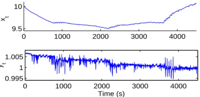
0 1000 2000 3000 4000 9.5 10 x t 0 1000 2000 3000 4000 0.995 1 1.005 Time (s) y t
Fig. 1: Ratio of estimated xt(top) and yt(bottom)
with-out constraints to the one with constraints
t0= 0, the battery is often in a resting state, and the SoC
can be efficiently calculated using an OCV /SoC relation-ship. To verify the relevance of the proposed constraints, the unknown parameters are estimated based on the pre-sented MC-EM algorithm, using 200 particles, with as well as without constraints (14). When the estimation is per-formed without constraints, we impose an upper bound to xt to avoid numerical problems. Experimental results
show that both marginal likelihoods p(y0:T | Θ) are equal.
Table 1 shows the ratio of the parameters estimated with-out constraints to those estimated with constraints. It can be seen that, as shown in (12), D and σY are invariant in
both cases, whereas C is divided and σX is multiplied by
H = 10. For B, the ratio must be theoretically equal to H = 10. However, the experimental ratio is not fixed which is not surprising since B describes the evolution of the unknown xt. Figure 1 represents the ratio of estimated
xtand ytwithout constraints to the one with constraints.
The results show that the estimated ytis invariant whereas
xtis multiplied by H = 10. Thus, these results show that
under the proposed constraints, the penalized EM algo-rithm efficiently estimates the parameters and that the identifiability issue is resolved. It is noteworthy that, un-der constraints, the orun-der of magnitude of the estimated parameters and xtis physically accurate; for instance the
estimated state of charge xt∈ [0, 100].
6
Conclusion
This paper has addressed the identifiability of switching Markov state-space models where the unknown continu-ous state and the observations are scalars. We prove that, in case of an irreducible and aperiodic Markov chain, if a constraint relating the observations to the continuous state at a time t0 is available, the model parameters
be-come generally structurally identifiable. In order to verify
the relevance of this proposition, a comparison between ML parameters inference of a SMSSM, under and with-out the proposed constraints, is performed. The results show that, by considering the above constraints, the iden-tifiability issue is resolved and the EM algorithm works efficiently.
References
[1] S.M. Oh, J.M. Rehg, T. Balch, and F. Dellaert, “Learning and inferring motion patterns using para-metric segmental switching linear dynamic systems,” International Journal of Computer Vision, vol. 77, no. 1-3, pp. 103-124, 2008.
[2] M. Lammerding, P. Stephan, M. Trede, and B. Wil-fling, “Speculative bubbles in recent oil price dy-namics: evidence from a Bayesian Markov-switching state-space approach,” Energy Economics, vol. 36, pp. 491-502, 2013.
[3] R. Yoshida, S. Imoto, and T. Higuchi, “Estimating time-dependent gene networks from time series mi-croarray data by dynamic linear models with Markov switching,” Proceedings of the 2005 IEEE Computa-tional Systems Bioinformatics Conference, pp. 289-298, 2005.
[4] B.G. Leroux, “Maximum-likelihood estimation for hidden Markov models,” Stochastic Processes and their Applications, vol. 40, no. 1, pp. 127-143, 1992. [5] E. Walter, and Y. Lecourtier, “Unidentifiable
com-partmental models: what to do?,” Mathematical Bio-sciences, vol. 56, no. 1-2, pp. 1-25, 1981.
[6] P.V. Overschee, and B.D. Moor, “Subspace al-gorithms for the stochastic identification problem,” Proceedings of the 30th IEEE Conference on Deci-sion and Control, vol. 2, pp. 1321-1326, 1991. [7] R. Kalman, “Mathematical description of linear
dy-namical systems,” Journal of the Society for In-dustrial and Applied Mathematics Series A Control, vol. 1, no. 2, pp. 152-192, 1963.
[8] S. J. Yakowitz and J. D. Spragins, “On the identifia-bility of finite mixtures,” The Annals of Mathematical Statistics, vol. 39, pp. 209-214, Feb 1968.
[9] M. A. Tanner, Tools for statistical inference - Ob-served data and data augmentation methods, vol. 67, Springer-Verlag New York, 1991.
[10] A. Doucet and A. M. Johansen, “A tutorial on par-ticle filtering and smoothing: Fifteen years later,” Handbook of Nonlinear Filtering, vol. 12, pp. 656-704, 2009.
[11] G. Plett, “Extended Kalman filtering for battery management systems of LiPB-based HEV battery packs,” Journal of Power Sources, vol. 134, pp. 262-276, 2004.