Université de Montréal
Contributions à la fusion de segmentations et à l’interprétation sémantique d’images
par Lazhar Khelifi
Département d’informatique et de recherche opérationnelle Faculté des arts et des sciences
Thèse présentée à la Faculté des arts et des sciences en vue de l’obtention du grade de Philosophiæ Doctor (Ph.D.)
en Informatique
août, 2017
c
RÉSUMÉ
Cette thèse est consacrée à l’étude de deux problèmes complémentaires, soit la fusion de segmentation d’images et l’interprétation sémantique d’images. En effet, dans un pre-mier temps, nous proposons un ensemble d’outils algorithmiques permettant d’améliorer le résultat final de l’opération de la fusion. La segmentation d’images est une étape de prétraitement fréquente visant à simplifier la représentation d’une image par un ensemble de régions significatives et spatialement cohérentes (également connu sous le nom de « segments » ou « superpixels ») possédant des attributs similaires (tels que des parties cohérentes des objets ou de l’arrière-plan). À cette fin, nous proposons une nouvelle mé-thode de fusion de segmentation au sens du critère de l’Erreur de la Cohérence Globale (GCE), une métrique de perception intéressante qui considère la nature multi-échelle de toute segmentation de l’image en évaluant dans quelle mesure une carte de segmenta-tion peut constituer un raffinement d’une autre segmentasegmenta-tion. Dans un deuxième temps, nous présentons deux nouvelles approches pour la fusion des segmentations au sens de plusieurs critères en nous basant sur un concept très important de l’optimisation com-binatoire, soit l’optimisation multi-objectif. En effet, cette méthode de résolution qui cherche à optimiser plusieurs objectifs concurremment a rencontré un vif succès dans divers domaines. Dans un troisième temps, afin de mieux comprendre automatiquement les différentes classes d’une image segmentée, nous proposons une approche nouvelle et robuste basée sur un modèle à base d’énergie qui permet d’inférer les classes les plus probables en utilisant un ensemble de segmentations proches (au sens d’un certain cri-tère) issues d’une base d’apprentissage (avec des classes pré-interprétées) et une série de termes (d’énergie) de vraisemblance sémantique.
Mots clefs : Ensemble de segmentation, fusion, erreur de la cohérence globale (GCE), modèle de vraisemblance pénalisée, optimisation multi-objectif, prise de décision, segmentation sémantique d’image.
ABSTRACT
This thesis is dedicated to study two complementary problems, namely the fusion of image segmentation and the semantic interpretation of images. Indeed, at first we propose a set of algorithmic tools to improve the final result of the operation of the fusion. Image segmentation is a common preprocessing step which aims to simplify the image representation into significant and spatially coherent regions (also known as segments or super-pixels) with similar attributes (such as coherent parts of objects or the background). To this end, we propose a new fusion method of segmentation in the sense of the Global consistency error (GCE) criterion. GCE is an interesting metric of perception that takes into account the multiscale nature of any segmentations of the image while measuring the extent to which one segmentation map can be viewed as a refinement of another segmentation. Secondly, we present two new approaches for merging multiple segmentations within the framework of multiple criteria based on a very important concept of combinatorial optimization ; the multi-objective optimization. Indeed, this method of resolution which aims to optimize several objectives concurrently has met with great success in many other fields. Thirdly, to better and automatically understand the various classes of a segmented image we propose an original and reliable approach based on an energy-based model which allows us to deduce the most likely classes by using a set of identically partitioned segmentations (in the sense of a certain criterion) extracted from a learning database (with pre-interpreted classes) and a set of semantic likelihood (energy) terms.
Key words : Segmentation ensemble, fusion, global consistency error (GCE), pe-nalized likelihood model, multi-objective optimization, decision making, semantic image segmentation.
TABLE DES MATIÈRES
RÉSUMÉ . . . ii
ABSTRACT . . . iii
TABLE DES MATIÈRES . . . iv
LISTE DES TABLEAUX . . . viii
LISTE DES FIGURES . . . xi
LISTE DES APPENDICES . . . xix
LISTE DES SIGLES . . . xx
DÉDICACE . . . xxii REMERCIEMENTS . . . .xxiii CHAPITRE 1 : INTRODUCTION . . . 1 1.1 Contexte de recherche . . . 1 1.2 La segmentation d’images . . . 2 1.2.1 Définition . . . 2
1.2.2 Stratégies de segmentation d’images . . . 4
1.3 La fusion de segmentation d’images . . . 5
1.4 L’optimisation multi-objectif . . . 6
1.5 L’interprétation sémantique d’images segmentées . . . 8
1.6 Contributions . . . 9
1.7 Contributions . . . 9
1.8 Structure du document . . . 12
1.8.1 Plan de la thèse . . . 12
I Fusion de segmentations basée sur un modèle mono-objectif
17
CHAPITRE 2 : A NOVEL FUSION APPROACH BASED ON THE GLO-BAL CONSISTENCY CRITERION TO FUSING MULTIPLE
SEGMENTATIONS . . . 18
2.1 Introduction . . . 19
2.2 Proposed Fusion Model . . . 22
2.2.1 The GCE Measure . . . 22
2.2.2 Penalized Likelihood Based Fusion Model . . . 26
2.2.3 Optimization of the Fusion Model . . . 29
2.3 Generation of the Segmentation Ensemble . . . 32
2.4 Experimental Results . . . 34
2.4.1 Initial Tests Setup . . . 34
2.4.2 Performances and Comparison . . . 36
2.4.3 Discussion . . . 45
2.4.4 Computational Complexity . . . 48
2.5 Conclusion . . . 49
II Fusion de segmentations basée sur un modèle multi-objectif 51
CHAPITRE 3 : EFA-BMFM : A MULTI-CRITERIA FRAMEWORK FOR THE FUSION OF COLOUR IMAGE SEGMENTATION . 52 3.1 Introduction . . . 543.2 Multi-objective Optimization . . . 56
3.3 Generation of the Initial Segmentations . . . 58
3.4 Proposed Fusion Method . . . 61
3.4.1 Region-based VoI criterion . . . 61
3.4.2 Contour-based F-measure criterion . . . 62
3.4.3 Multi-objective function . . . 63
3.5 Experimental Tests and Results . . . 67
3.5.1 Data set and benchmarks . . . 67
3.5.2 Initial tests . . . 69
3.5.3 Performance measures and results . . . 72
3.5.4 Comparison of medical image segmentation . . . 73
3.5.5 Comparison of Segmentation Methods for Aerial Image Seg-mentation . . . 83
3.5.6 Algorithm complexity . . . 85
3.5.7 Discussion . . . 88
3.6 Conclusion . . . 91
CHAPITRE 4 : A MULTI-OBJECTIVE DECISION MAKING APPROACH FOR SOLVING THE IMAGE SEGMENTATION FUSION PROBLEM . . . 92
4.1 Introduction . . . 93
4.2 Literature Review . . . 95
4.3 Proposed Fusion Model . . . 97
4.3.1 Multi-objective Optimization . . . 97
4.3.2 Segmentation Criteria . . . 99
4.3.3 Multi-Objective Function Based-Fusion Model . . . 102
4.3.4 Optimization Algorithm of the Fusion Model . . . 104
4.3.5 Decision Making With TOPSIS . . . 106
4.4 Segmentation Ensemble Generation . . . 106
4.5 Experimental Results and Discussion . . . 111
4.5.1 Initial Tests . . . 111
4.5.2 Evaluation of the Performance . . . 112
4.5.3 Sensitivity to parameters . . . 116
4.5.4 Other Results and Discussion . . . 122
4.5.5 Discussion and Future Work . . . 125
4.6 Conclusion . . . 130
III Interprétation sémantique d’images
132
CHAPITRE 5 : MC-SSM : NONPARAMETRIC SCENE PARSING VIA AN ENERGY BASED MODEL . . . 1335.1 Introduction . . . 134
5.2 Related Work . . . 135
5.3 Model Description . . . 137
5.3.1 Regions Generation . . . 137
5.3.2 Geometric Retrieval Set . . . 139
5.3.3 Region Features . . . 142
5.3.4 Image labeling . . . 145
5.4 Experiments . . . 148
5.4.1 Datasets . . . 148
5.4.2 Evaluation Metrics . . . 149
5.4.3 Results and Discussion . . . 150
5.4.4 Computation Time . . . 157
5.5 Conclusion . . . 161
CHAPITRE 6 : CONCLUSION GÉNÉRALE ET PERSPECTIVES . . . . 162
6.1 Sommaire des contributions . . . 162
6.2 Limites et orientations futures de la recherche . . . 163
LISTE DES TABLEAUX
2.1 Average performance, related to the PRI metric, of several region-based segmentation algorithms (with or without a fusion model strategy) on the BSD300, ranked in the descending order of their PRI score (the higher value is the better) and considering only the (published) segmentation methods with a PRI score above 0.75. . . 38 2.2 Average performance of diverse region-based segmentation algorithms
(with or without a fusion model strategy) for three different performances (distance) measures (the lower value is the better) on the BSD300. . . . 41 2.3 Comparison of scores between the GCEBFM and the MDSCCT
algo-rithms on the 300 images of the BSDS300. Each value points out the number of images of the BSDS300 that obtain the best score. . . 46 2.4 Average CPU time for different segmentation algorithms. . . 49 3.1 Performance of several segmentation algorithms (with or without a
fu-sion model strategy) for three different performance measures : VoI, GCE and BDE (lower is better), on the BSDS300. . . 74 3.2 Performance of several segmentation algorithms (with or without a
fu-sion model strategy) for the PRI performance measure (higher is better) on the BSDS300. . . 75 3.3 Performance of several segmentation algorithms (with or without a
fu-sion model strategy) for three different performance measures : VoI, GCE and BDE (lower is better), on the BSDS500. . . 76 3.4 Performance of several segmentation algorithms (with or without a
fu-sion model strategy) for the PRI performance measure (higher is better) on the BSDS500. . . 77
3.5 Boundary benchmarks on the aerial image segmentation dataset (ASD). Results obtained for different segmentation methods (with or without the fusion model strategy). The figure shows the F-measures (higher is better) when choosing an optimal scale for the entire dataset (ODS) or per image (OIS). . . 86 3.6 Fusion segmentation models and complexity. . . 86 3.7 Average CPU time for different segmentation algorithms for the BSDS300. 88 3.8 Comparison of scores between the EFA-BMFM and other segmentation
algorithms for the 300 images of the BSDS300. Each value indicates the number of images of the BSDS300 which obtain the best score. . . 89 4.1 Benchmarks on the BSDS300. Results for diverse segmentation
algo-rithms (with or without a fusion model strategy) in terms of : the VoI, the GCE (the lower value is the better) and the PRI (the higher value is the better) and a boundary measure : the BDE (the lower value is the better)117 4.2 Benchmarks on the BSDS500. Results for diverse segmentation
algo-rithms (with or without a fusion model strategy) in terms of : the VoI, the GCE (the lower value is the better) and the PRI (the higher value is the better) and a boundary measure : the BDE (the lower Value is the better). . . 120 4.3 Influence of the value of parameter Kmax
1 (average performance on the
BSDS300). . . 123 4.4 The Value of VoI, GCE, PRI and BDE as a function of the used
crite-rion ; single-critecrite-rion (either F-Measure and GCE) and the tow combined criteria (GCE+F-measure) . . . 126 4.5 Average CPU time for different segmentation algorithms on the BSDS300.129 5.1 Summary of the combined criteria used in our Model. . . 147 5.2 Performance of our model on the MSRC-21 segmentation dataset in
terms of global per-pixel accuracy and average per-class accuracy (hi-gher is better). . . 152
5.3 Accuracy of segmentation for the MSRC 21-class dataset. Confusion matrix with percentages row-normalized. The overall per-pixel accuracy is 75%. . . 153 5.4 Performance of our model on the Stanford background dataset (SBD) in
terms of global per-pixel accuracy and average per-class accuracy (hi-gher is better). . . 155 5.5 Accuracy of segmentation for the SBD dataset. Confusion matrix with
percentages row-normalized. The overall per-pixel accuracy is 68%. . . 156 5.6 Performance of our model using single and multiple criteria (on the
LISTE DES FIGURES
1.1 De gauche à droite ; une image couleur, sa segmentation en régions (R1,
R2et R3) et sa représentation en classes (c1: arrière-plan et c2: rondelle). 4
1.2 Fusion de segmentations. . . 7 1.3 Quelques défis liés à l’interprétation sémantique d’images : la
déforma-tion (a), la confusion d’arrière-plan (b), l’occultadéforma-tion (c), les condidéforma-tions d’éclairage (d), la variation de point de vue (e), la variation d’échelle (f), et la variation intra-classe (g). . . 16 2.1 Examples of initial segmentation ensemble and fusion results (Algo.
GCE-Based Fusion Model). Three first rows ; Results of K-means clus-tering for the segmentation model presented in Section 2.3. The forth row ; Input image chosen from the Berkeley image dataset and final seg-mentation given by our fusion framework. . . 27 2.2 Example of fusion convergence result on three various initializations for
the Berkeley image (n0187039). Left : initialization and Right :
segmen-tation result after 8 iterations of our GCEBFM fusion model. From top to bottom, the original image, the two input segmentations (from the seg-mentation set) which have the best and the worst GCE⋆β value and one non informative (or blind) initialization. . . 30 2.3 Progression of the segmentation result (from lexicographic order) during
the iterations of the relaxation process beginning with a non informative (blind) initialization. . . 30 2.4 An example of segmentation solutions generated for different values of
R (β= 0.01), from top to bottom and left to right, R = {1.2, 2.2, 3.2, 4.2},
2.5 Example of fusion result using respectively L = 5, 10, 30, 60 input mentations (i.e., 1, 2, 6, 12 color spaces). We can also compare the seg-mentation results with the segseg-mentation maps given by a simple K-means algorithm (see examples of segmentation maps in the segmen-tation ensemble at Fig. 2.1). . . 35 2.6 Plot of the average number of different regions obtained for each
seg-mentation (of the BSD300) as a function of the value of R. . . 37 2.7 Example of segmentations obtained by our algorithm GCEBFM on
seve-ral images of the Berkeley image dataset (see also Tables 2.1 and 2.2 for quantitative performance measures and "http ://www.etud.iro.umontreal. ca/∼khelifil/ResearchMaterial/gcebfm.html" for the segmentation results on the entire dataset). . . 39 2.8 Example of segmentations obtained by our algorithm GCEBFM on
seve-ral images of the Berkeley image dataset (see also Tables 2.1 and 2.2 for quantitative performance measures and "http ://www.etud.iro.umontreal. ca/∼khelifil/ResearchMaterial/gcebfm.html" for the segmentation results on the entire dataset). . . 40 2.9 Distribution of the PRI metric, the number and the size of regions over
the 300 segmented images of the Berkeley image dataset. . . 42 2.10 From lexicographic order, progression of the PRI (the higher value is
better) and VoI, GCE, BDE metrics (the lower value is better) according to the segmentations number (L) to be fused for our GCEBFM algorithm. Precisely, for L = 1, 5, ..., 60 segmentations (by considering first, one K-means segmentation (according to the RGB color space) and then by considering five segmentation for each color space and 1, 2, . . ., 12 color spaces). . . 44 2.11 First row ; three natural images from the BSD300. Second row ; the result
of segmentation provided by the MDSCCT algorithm. Third row ; the result of segmentation obtained by our algorithm GCEBFM. . . 47
3.1 The weighted formula approach (WFA). . . 59 3.2 Examples of initial segmentation set and combination result (output of
Algorithm 1). (a) Results of K-means clustering. (b) Input image ID 198054 selected from the Berkeley image dataset. (c) Final segmenta-tion given by our fusion framework. (d) Contour superimposed on the colour image. . . 60 3.3 Two images from the BSDS300 (a) and its ground truth boundaries (b).
Segmentation results obtained by our EFA-BMFM are shown in (c). . . 65 3.4 Example of fusion convergence result for three various initializations.
(a) Berkeley image ID 229036 and its ground-truth segmentations. (b) A non informative (or blind) initialization. (c) The worst input segmen-tation. (d) The best input segmentation (from the segmentation set) se-lected by the entropy method (see Section 3.4.4). (e), (f) and (g) seg-mentation results after 10 iterations of our EFA-BMFM fusion model (resulting from (b), (c) and (d), respectively). . . 70 3.5 Average error of different initialization methods (for the probabilistic
Rand index (PRI) performance measure) on the BSDS300. . . 71 3.6 Progression of the segmentation result as a function of the number of
segmentations (L) to be fused for the EFA-BMFM algorithm. More pre-cisely, for L= 12, 24, 36, 48 and 60 segmentations. . . 71 3.7 Progression of the VoI, (lower is better) and the PRI (higher is better)
according to the segmentation number (L) to be fused for our proposed EFA-BMFM algorithm (on the BSDS500). Precisely, for L = 1, 12, 24, 36, 48 and 60 segmentations. . . 76 3.8 A sample of results obtained by applying our proposed algorithm to
images from the Berkeley dataset compared to other algorithms. From left to right : original images, FCR [2], SCKM [3], MD2S [4], GCEBFM [5], MDSCCT [6] and our method (EFA-BMFM). . . 78 3.9 Additional segmentation results obtained from the BSDS300. . . 79
3.10 Best and worst segmentation results (in the PRI sense) obtained from the BSDS300. First column : (a) image ID 167062 and (b) its segmentation result (PRI=0.99). Second column : (c) image ID 175043 and (d) its segmentation result (PRI = 0.37). . . 80 3.11 Distribution of the BDE, GCE, PRI and VoI measures over the 300
seg-mented images of the BSDS300. . . 81 3.12 Distribution of the number and size of regions over the 300 segmented
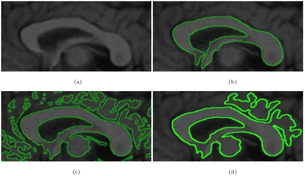
images of the BSDS300. . . 82 3.13 Comparison of two region-based active contour models on a brain MRI.
(a) original image. (b) segmentation of the RLSF model [7]. (c) segmen-tation of the global active contour model [7]. (d) segmensegmen-tation achieved by our EFA-BMFM model. . . 83 3.14 Comparison of two segmentation methods on segmenting a real cornea
image. (a) original image of size 256×256. (b) detection using the FGM method [8] (5000 iterations). (c) detection using the DMD method [9] (5 iterations). (d) detection resulting from our EFA-BMFM model (10 iterations). . . 84 3.15 A sample of results obtained by applying our algorithm to images from
the aerial image dataset [10] compared to other popular segmentation algorithms (gPb-owt-ucm [11], Felz-Hutt (FH) [12], SRM [13], Mean shift [14], JSEG [15], FSEG [16] and MSEG [17]). The first row shows six example images. The second row overlays segment boundaries gene-rated by four subjects, where the darker pixels correspond to the boun-daries marked by more subjects. The last row shows the results obtained by our method (EFA-BMFM). . . 87 3.16 Convergence analysis. (a) input image ID 187039 selected from the BSDS300.
(b) change of the segmentation map of our EFA-BMFM fusion model starting from a blind (or non informative) initialization. (c) evolution of the consensus energy function along the number of iterations of the EFA-BMFM. . . 90
4.1 Pareto frontier of a multi-objective problem in case of a minimization. . 99 4.2 Four images from the BSDS300 and their ground truth boundaries. The
images shown in the last column are obtained by our MOBFM fusion model. . . 101 4.3 A set of initial segmentations and the final fusion result achieved by
MOBFM algorithm. From top to bottom ; Four first rows ; K-means clus-tering results for the segmentation model detailed in Section 4.4. Fifth row : Natural image from the BSDS500 and final segmentation map re-sulting of our fusion algorithm. . . 103 4.4 First row ; a natural image (n0176035) from the BSDS500. Second row ;
the Pareto frontier generated by the MOBFM algorithm (cf. Algorithm 1). 108 4.5 Graphical representation of TOPSIS (technique for order performance
by similarity to ideal solution). . . 109 4.6 The ordered set of solutions, i.e, segmentations, belonging to the
Pareto-front ; The boxes marked in blue, black and yellow indicate, respectively, the solution which has the minimum GCE⋆γscore, the solution which has the maximum Fα score and the best solution chosen automatically by
TOPSIS among these different solutions belonging to the Pareto frontier (cf, Fig. 4.4). . . 109 4.7 Complexity values obtained on five images of the BSDS300 [18]. From
left to right, value of complexity = 0.450, 0.581, 0.642, 0.695, 0.796 corresponding to the number of classes (k) (with the three different va-lue of Kmax: Kmax
1 , K2max and K3max) of the k-means clustering algorithm
res-pectively to (5, 4, 2), (6, 5, 2), (7, 6, 2), (8, 6, 2), (9, 7, 3) in the k-means segmentation model. . . 112
4.8 Fusion convergence result on six different initializations for the Berkeley image n0247085. Left : initialization and Right : result after 11 iterations of our MOBFM fusion model. From top to bottom, the original image, two blind initialization, the input segmentation which have the J/6 = 10 −th best GCE⋆γ score, the input segmentation which have the J/2 =
30−th best GCE⋆γscore and the two segmentations which have the worst
and the best score GCE⋆γ. . . 113 4.9 First row ; a natural image (n0134052) from the BSDS300. Second and
third row ; evolution of the resulting segmentation map (0-th, 1-st, 2-nd, 4-th, 6-th, 8-th, 11-th, 20-th, 40-th, 80-th) (from lexicographic order) along the iterations of the relaxation process starting from a blind initia-lization. . . 114 4.10 First and second row ; evolution of the resulting segmentation map (0-th,
1-st, 2-nd, 4-th, 6-th, 8-th, 11-th, 20-th, 40-th, 80-th), from lexicographic order along the iterations of the relaxation process starting from the ini-tial segmentation which have the best GCE⋆γ score. Third row ; evolution of the Mean GCE value and the F-Measure value along iterations. . . . 115 4.11 From top to bottom, distribution of the PRI measure, the number and the
size of regions over the 300 segmented images of the BSDS300 database. 118 4.12 Example of fusion results using respectively J = 5, 10, 15, 20, 25, 30,
35, 40, 45, 50, 55, 60 input segmentations (i.e., 1, 2, 3, 4, 5, 6, 7, 8, 9, 10, 11, 12 color spaces). . . 119 4.13 From lexicographic order, evolution of the PRI (higher is better) and
VoI, GCE, BDE measures (lower is better) as a function of the number of segmentations (J) to be combined for our MOBFM algorithm. More precisely for J = 1, 5, 10, 15, 20, . . ., 60 segmentations, by considering first, one K-mean segmentation and then by considering five segmenta-tions for each color space and 1, 2, 3, . . ., 12 color spaces. . . 121 4.14 Example of segmentation solutions obtained for different values of α,
4.15 Example of segmentation solutions obtained for different values of Q, from top to bottom and left to right, Q={0.2, 1, 2, 4.2}. . . 124 4.16 Example of segmentation results obtained by our algorithm MOBFM on
four images from the BSDS300 compared to other algorithms with or without a fusion model strategy (FCR [2], GCEBFM [5] and CTM [19]. 126 5.1 System overview. Given an input image (a), we generate its set of regions
with the GCEBFM algorithm (b), we retrieve similar images from the full dataset (c) using the GCE criterion, we extract different features both for the input image (f) and the retrieved images (d). Based on the labeled segmentation corpus (e), a single class label is assigned to each region (g) using energy minimization based on the ICM. . . 138 5.2 Regions generation by the GCEBFM algorithm [20]. (a) input image. (b)
examples of initial segmentation ensemble. (c) segmentation result. . . . 140 5.3 Generation of the OCLBP histogram for each region. (a) The regions
map of the input image. (b) Estimation of LBP value of a center pixel from one color channel based on neighborhoods from another channel [see (5.4)]. (c)-(d) Estimation, for each pixel X, of the Nbbin descriptor
q= 5 in the cube of pair channels. Each LbpR−GX ,LbpR−BX, LbpG−
BX value associated with each pixel contained in a squared neighborhood
region of size 7 × 7 centered at a pixel X, increments (+1) a particular bin. (e) OCLBP histogram of each region. . . 147 5.4 Example of segmentation result obtained by our algorithm MC-SSM on
an input image from the MSRC-21 compared to other algorithms. . . . 154 5.5 Example results obtained by our MC-SSM model on the MSRC-21
da-taset (for more clarity, we have superimposed textual labels on the resul-ting segmentations). . . 154 5.6 Example results of failures on the MSRC-21 dataset. Top : query image,
5.7 Effects of varying the retrieval set size K for the MSRC-21 dataset ; shown are the overall per-pixel accuracy and the average per-class
ac-curacy. . . 158
5.8 Evolution of the overall pixel accuracy and the average global per-class accuracy along the number of iterations of the proposed MC-SSM starting from a random initialization on the MSRC-21 dataset. . . 160
I.1 Color input image from the MSRC-21 Dataset. . . i
I.2 Result of local binary pattern (LBP), with r = 2 and P = 9. . . ii
I.3 Result of local binary pattern (LBP), with r = 2 and P = 16. . . ii
I.4 Result of opponent color local binary pattern (OCLBP), with r = 1 and P= 9 (red-green, red-blue and green-blue). . . iii
I.5 Result of opponent color local binary pattern (OCLBP), with r = 2 and P= 16 (red-green, red-blue and green-blue). . . iii
I.6 Result of opponent color local binary pattern (OCLBP), with r = 1 and P= 9 (green-red, blue-red and blue-green). . . iv
I.7 Result opponent color local binary pattern (OCLBP), with r = 2 and P= 16 (green-red, blue-red and blue-green). . . iv
I.8 Result of Laplacian operator (LAP), with r = 1 and P = 9. . . v
I.9 Result of Laplacian operator (LAP), with r = 2 and P = 16. . . v
LISTE DES APPENDICES
Annexe I : Opérateurs de quantification de textures . . . i Annexe II : Échéancier de la thèse . . . vi
LISTE DES SIGLES
ACA Average per-Class Accuracy ASD Aerial image Segmentation Dataset BCE Bidirectional Consistency Error BDE Boundary Displacement Error BSD Berkeley Segmentation Dataset CPU Central Processing Unit
CRF Conditional Random Field CNNs Convolutional Neural Networks
DMD Multiplicative and Difference Model
EFA-BMFM Multi-criteria Fusion Model Based on the Entropy-Weighted Formula Approach
EM Expectation Maximization ESE Exploration/Selection/Estimation FGM Fast Global Minimization
FS Feasible Solutions
GCE Global Consistency Error
GCEBFM Global Consistency Error Based Fusion Model GPA Global per-Pixel Accuracy
GPU Graphic Processor Unit
HOG Histogram of Oriented Gradients ICM Iterative Conditional Modes KNN K-Nearest Neighbor
LBP Local Binary Pattern LMO LabelMe Outdoor
LSD Line Segment Detector LRE Local Refinement Error
MCDM Multi-Criteria Decision Making
MC-SSM Multi-Criteria Semantic Segmentation Model ML Maximum Likelihood
MO Multi-objective Optimization
MOBFM Multi-objective Optimization Based Fusion Model MRF Markov Random Fields
MRI Magnetic Resonance Imaging
MSRC Microsoft Research Cambridge Dataset OCLBP Opponent Color Local Binary Pattern
ODS Optimal Data set Scale OIS Optimal Image Scale PRI Probabilistic Rand Index PTA Pareto Approach
RI Rand Index
RLSF Region-based model via Local Similarity Factor SA Simulated Annealing
SBD Stanford Background Dataset SIFT Scale-Invariant Feature Transform
TOPSIS Technique for Order Performance by Similarity to Ideal Solution VoI Variation of Information
Je dédie cette thèse à :
Ma mère.
Pour son appui indéfectible durant mes études. Je n’oublie pas ses énormes sacrifices.
L’âme de mon cher père.
A mes frères.
A mes soeurs.
REMERCIEMENTS
À l’occasion du présent travail de doctorat je désire remercier le Ministère de l’ensei-gnement supérieur tunisien et l’Université de Montréal pour avoir co-financé ce travail de recherche à travers plusieurs bourses d’excellence.
Je tiens à exprimer en tout premier lieu mon immense gratitude à mon directeur de thèse le professeur Max Mignotte, d’avoir accepté de diriger mes travaux de recherche, de faire confiance à mes compétences et de m’offrir une grande autonomie. Je le re-mercie aussi pour son encadrement et pour son expertise dans le domaine segmentation d’images, ainsi que pour la grande disponibilité dont il a fait preuve tout au long du déroulement de cette thèse.
Je veux remercier également les membres du jury qui ont bien voulu me faire l’hon-neur de juger cette thèse.
Finalement, je remercie tous les professeurs qui ont contribué à ma formation uni-versitaire.
CHAPITRE 1
INTRODUCTION
1.1 Contexte de recherche
La vision par ordinateur est une branche de l’intelligence artificielle qui permet à une machine de comprendre ce qu’elle « voit » lorsqu’on la connecte à une ou plu-sieurs caméras. En d’autres termes, c’est un traitement automatisé des informations vi-suelles par ordinateur. Cette discipline scientifique étant très vaste, elle englobe d’autres sous-domaines tels que le traitement d’images qui est une discipline riche et qui donne lieu à une profusion de travaux académiques et industriels chaque année. En effet, les connaissances en la matière s’appliquent de nos jours dans plusieurs contextes comme la retouche d’images, la reconnaissance faciale, l’analyse de scènes routières, l’imagerie multi-spectrale, la reconnaissance de l’écriture, l’imagerie médicale, etc. Cette richesse s’explique par l’importance de l’analyse, l’extraction de l’information et la compréhen-sion de l’image. À cet égard, plusieurs techniques et méthodes ont été proposées afin de trouver les solutions adéquates pour résoudre les problèmes qui se présentent pendant les différentes phases de traitement de l’image :
• La phase de prétraitement (traitements photométriques et colorimétriques, réduc-tion de bruit, restauraréduc-tion d’images, etc.), qui permet une meilleure visualisaréduc-tion de l’image, facilitant ainsi les traitements ultérieurs ;
• La phase de segmentation, qui consiste à partitionner l’image en un ensemble de régions connexes et cohérentes ;
• La phase de quantification (description de forme, caractéristiques géométriques d’un objet, etc.), qui a pour but de fournir des indices quantitatifs ou géométriques.
Dans cette thèse, nous nous intéressons, dans un premier temps, à la phase de seg-mentation. En effet, la segmentation d’image est une étape primordiale qui consiste à
regrouper les pixels de l’image en différentes régions selon des critères de ressemblance prédéfinis (il peut s’agir, par exemple, de séparer les objets du fond). Cette opération dite de bas niveau permet d’obtenir une représentation simplifiée de l’image. Elle n’est pas considérée comme un but, mais comme un moyen efficace qui permet ensuite d’effectuer des tâches de plus haut niveau visant à analyser le contenu de l’image.
La résolution de problèmes de segmentation d’images nécessite l’implémentation d’un algorithme qui permet de diviser l’image en zones de régions homogènes. Cepen-dant, les expériences en segmentation nous ont montré qu’il est difficile d’obtenir un tel résultat en utilisant un algorithme classique de segmentation. À cette fin, au lieu de concevoir un algorithme de segmentation très compliqué, nous proposons dans ce tra-vail une autre méthodologie qui consiste à segmenter l’image avec des algorithmes très simples, mais très différents, puis à fusionner les résultats (ou cartes de segmentation) à l’aide d’une procédure de fusion calculant une sorte de moyennage de segmentation pour générer une segmentation finale plus robuste. Suivant cette stratégie, nous propo-sons deux modèles de fusion de segmentation d’image, soit le modèle mono-objectif, basé sur un seul critère, et le modèle multi-objectif, basé sur différents critères et sur le concept de l’optimisation multi-objectif.
Notre démarche s’inspirant de la logique et de la perception humaine, nous nous pen-chons dans un deuxième temps sur un autre problème, soit l’interprétation sémantique d’images. À cet égard, nous présentons un nouveau système permettant d’identifier au-tomatiquement les différentes régions d’une image segmentée.
1.2 La segmentation d’images 1.2.1 Définition
La segmentation d’images est une étape de prétraitement fréquente visant à simpli-fier la représentation d’image par un ensemble de régions significatives et spatialement cohérentes (aussi appelées « superpixels ») possédant des attributs similaires (tels que des parties cohérentes d’un même objet ou de l’arrière-plan). Cette tâche de vision de
bas niveau, qui modifie la représentation d’une image en quelque chose de plus facile à analyser, est souvent l’étape préliminaire et également critique dans le développement de nombreux algorithmes de compréhension de l’image et des systèmes de vision par or-dinateur tels que les problèmes de reconstruction [21] ou la localisation/reconnaissance d’objet 3D [22, 23].
La segmentation consiste à partitionner une image I en n régions différentes R1, ..., Rn.
Les régions obtenues doivent respecter les propriétés d’homogénéité. Mathématique-ment, soit P(Ri) le prédicat logique qui définit l’homogénéité d’une région Ri. Ce
prédi-cat est défini formellement par l’équation suivante :
P(Ri) =
vrai si Ri est homog´ene
f aux sinon (1.1)
Pour valider un résultat de segmentation, les régions générées par un algorithme doivent respecter les conditions suivantes [1] :
• Recouvrement : chaque pixel de l’image doit appartenir à une région Riet l’union
de toutes les régions correspond à l’image entière Sn
i=1Ri= I.
• Connexité : les pixels qui appartiennent a une région doivent être connectés, plus précisément pour toute paire de pixels p et q d’une région Ri , il est possible de
tracer un chemin de p vers q en ne passant que par des pixels de la région Ri[24]
Riforme un ensemble connexe ∀i = 1,2,...n.
• Disjonction : aucun pixel ne fait partie de deux régions différentes à la fois RiTRj= ∅ ∀i, j |i 6= j.
• Satisfiabilité : chaque région doit satisfaire un prédicat d’homogénéité P P(Ri) = V RAI ∀i = 1,2,...n.
• Segmentabilité : un même prédicat ne se réalise pas pour l’union de deux régions adjacentes
P(RiSRj) = FAU X ∀i, j |i 6= j et Ri, Rjétant adjacents dans I.
D’un point de vue algorithmique, une région est un groupe de pixels connectés entre eux avec des propriétés similaires, par contre, une classe est un ensemble de pixels qui possèdent des caractéristiques texturales similaires, la figure 1.1 montre la différence entre ces deux notions.
FIGURE 1.1 : De gauche à droite ; une image couleur, sa segmentation en régions (R1,
R2et R3) et sa représentation en classes (c1: arrière-plan et c2: rondelle).
1.2.2 Stratégies de segmentation d’images
Une pléthore de méthodes de segmentation basées sur les régions a été proposée afin de résoudre le problème difficile de la segmentation non supervisée d’images natu-relles texturées. La plupart de ces méthodes exploitent une première étape d’extraction de paramètres, pour caractériser chaque région texturée significative à segmenter, sui-vie d’une technique de classification, qui permet de regrouper selon des critères ou des stratégies différentes des régions spatialement cohérentes partageant des attributs simi-laires. Pendant des années, les recherches en segmentation se sont concentrées sur des caractéristiques plus sophistiquées d’extraction de caractéristiques et des techniques de classification plus élaborées. Ces travaux ont amélioré de façon significative les résul-tats finaux de segmentation, mais ont généralement augmenté la complexité du modèle et/ou de calcul. Ces méthodes comprennent des modèles de segmentation qui exploitent
directement des systèmes de regroupement (« clustering ») [2, 3, 19, 25] en utilisant la modélisation par mélange de gaussiennes [26], l’approche de classification floue [27,28], les ensembles flous [29] ou, après une approche de dé-texturation [3, 4, 6]), le « mean-shift » ou plus généralement des procédures basées sur la recherche des modes d’une distribution [30], les méthodes de ligne de partage d’eaux [31] ou les stratégies de crois-sance de la région [32], les modèles de codage et de compression avec perte [31, 33], la transformée en ondelettes [34], les champs aléatoires de Markov (MRF) [35–37], l’ap-proche Bayésienne [38], l’apl’ap-proche basée sur le texton [39] ou les modèles basés sur le graphe [12,40,41], les méthodes variationnelles ou de l’ensemble du niveau [39,42–45], les modèles de surfaces déformables [46], de contour actif [47] (avec approche basée sur le partitionnement de graphe [48]) ou les techniques basées sur les courbes [49], la technique de seuillage non supervisée itérative [50, 51], l’algorithme génétique [52], les cartes auto-organisatrices [53], la technique de l’apprentissage de variétés [54], l’ap-proche basée sur la topologie [55], les objets symboliques [56] et la classification spec-trale [57], etc. pour en citer que quelques-uns.
1.3 La fusion de segmentation d’images
Une variante récente et efficace de segmentation consiste à combiner ou fusionner plusieurs cartes de segmentation grossièrement et rapidement estimées de la même scène et associée à un modèle de segmentation1 simple, pour obtenir une segmentation finale
améliorée. Au lieu de chercher le meilleur algorithme de segmentation avec ses para-mètres internes optimaux, ce qui est difficile si l’on tient compte des différents types d’images existantes, cette stratégie privilégie la recherche d’un modèle de fusion de seg-mentations, ou plus précisément, la recherche du critère le plus efficace pour fusionner de multiples segmentations.
1Ces cartes de segmentations destinées à être fusionnées peuvent être générées par différents algo-rithmes (idéalement complémentaires) ou par le même algorithme ayant différentes valeurs des paramètres internes ou graines (pour les méthodes stochastiques), ou en utilisant des caractéristiques texturales diffé-rentes et appliquées à une image d’entrée éventuellement exprimée dans différents espaces de couleurs ou transformations géométriques (par exemple, facteur d’échelle, inclinaison, etc.) ou par d’autres moyens.
La combinaison de plusieurs segmentations peut constituer un cas particulier du pro-blème d’ensemble de classifieurs, c’est-à-dire le concept qui combine plusieurs méthodes de classification pour améliorer le résultat final de classification (et qui fut d’abord ex-ploré dans le domaine de l’apprentissage machine [58–60]). En effet, l’ordonnancement spatial est un aspect distinctif des données d’une image et la segmentation d’images est donc un processus de regroupement des données spatialement indexées. Par conséquent, le groupement des pixels doit non seulement tenir compte de la similitude de leur carac-téristique (couleur, texture, etc.), mais aussi de leur cohérence spatiale. Il est intéressant de noter que ce problème de fusion de segmentation ou segmentation d’ensemble peut également être considéré comme étant un cas particulier d’un problème de débruitage dans lequel chaque segmentation à fusionner est en fait une solution bruitée ou une ob-servation. L’objectif final est donc de trouver une solution de segmentation débruitée, qui serait en fait un consensus ou un compromis (en termes de clusters, de niveau de détails, de précision de contour, etc.) de toutes les segmentations. En un sens, la segmen-tation finale fusionnée représente la moyenne de toutes les segmensegmen-tations individuelles à combiner selon un critère bien défini. Quand cette stratégie a d’abord été introduite en [61] [62], toutes les segmentations à fusionner devaient contenir le même nombre de régions. Un peu plus tard, cette stratégie fut utilisée sans cette restriction, avec un nombre arbitraire de régions [2, 63]. Depuis ces travaux novateurs, cette fusion de mul-tiples segmentations de la même scène, pour obtenir un résultat de segmentation plus fiable et précis, est maintenant effectuée selon plusieurs stratégies et/ou des critères bien définis (Figure 1.2).
1.4 L’optimisation multi-objectif
Le problème de segmentation d’image est souvent formalisé sous la forme d’un pro-blème d’optimisation. Un propro-blème d’optimisation est défini, généralement, par un es-pace de recherche S et une fonction objectif f . Le but est de trouver la solution de meilleure qualité. Suivant le problème posé, nous cherchons soit le minimum soit le maximum de la fonction f [64]. Formellement, un problème d’optimisation peut être
représenté de la manière suivante :
min f(−→x) (function à optimiser) avec −→g(−→x) 6 0 m contraintes d’inégalités
et −→h(−→x) = 0 p contraintes d’égalités (1.2)
où −→x ∈ ℜn, −→g(−→x) ∈ ℜm,−→h(−→x) ∈ ℜp. Les vecteurs −→g(−→x) et −→h(−→x) représentent respectivement m contraintes d’inégalité et p contraintes d’égalité. Cet ensemble de contraintes permet de délimiter un espace restreint de recherche de la solution optimale pour un certain problème. L’optimisation mono-objectif consiste à maximiser (ou mini-miser) une seule fonction objective par rapport à un ensemble de paramètres. Cependant, dans le cas multi-objectif, on cherche à satisfaire plusieurs objectifs souvent contradic-toires devant être simultanément maximisés ou minimisés . Par conséquent, l’augmenta-tion d’un objectif entraîne une diminul’augmenta-tion de l’autre objectif. Mathématiquement, dans le cas de la minimisation le problème s’écrit de la manière suivante :
min −→f (−→x) (k function à optimiser) avec −→g(−→x) 6 0 m contraintes d’inégalités
et −→h(−→x) = 0 p contraintes d’égalités (1.3)
où −→x ∈ ℜn,−→f (−→x) ∈ ℜk, −→g(−→x) ∈ ℜm,−→h(−→x) ∈ ℜp et f représente un vecteur qui regroupe k fonctions objectif.
1.5 L’interprétation sémantique d’images segmentées
L’interprétation sémantique d’images segmentées, également appelée la classifica-tion d’objets visuels, vise à diviser et étiqueter l’image en régions sémantiques ou ob-jets, par exemple ; montagne, ciel, bâtiment, arbre, etc. Bien que cette tache soit triviale pour un être humain, elle est considérée comme l’un des problèmes les plus difficiles dans le domaine de la vision par ordinateur. Une des raisons de cette difficulté vient du fait que certains défis importants doivent être pris en compte afin d’avoir un bon résultat d’étiquetage, tels que ; la variation de point de vue, la variation d’échelle, la
déforma-tion, l’occultadéforma-tion, les conditions d’éclairage, la confusion d’arrière-plan et la variation intra-classe2(voir Figure 1.3).
1.6 Contributions 1.7 Contributions
Le but de cette thèse est l’étude de deux problèmes complémentaires, soit la segmen-tation (en régions) et l’interprésegmen-tation sémantique d’images. La nature mal posée de ces deux problèmes et la proposition de nouveaux modèles non-paramétriques de minimisa-tion d’énergie à base de fusion rendent ce travail distinct de la majorité des méthodes qui ont utilisé des approches purement paramétriques ou basé sur l’apprentissage machine. Le travail réalisé dans cette thèse se divise essentiellement en trois parties :
Fusion de segmentations mono-objectif :
L’approche de fusion de différentes segmentations d’une même scène afin d’obte-nir un résultat de segmentation plus précis a été proposée récemment selon plusieurs stratégies ou critères. Nous pouvons mentionner le modèle de fusion introduit dans [2] qui fusionne un ensemble de segmentations en minimisant la dispersion (ou l’inertie) des étiquettes obtenues localement autour de chaque pixel de l’image en exécutant sim-plement une procédure de fusion à base de l’algorithme des k-moyennes. De la même manière, on peut également citer le modèle proposé dans [72] qui suit la même idée, mais au sens de l’inertie pondérée en exploitant cette fois l’algorithme des k-moyennes flou. Cette fusion de segmentations a également été réalisée en utilisant la version pro-babiliste du critère Rand (PRI) [70] grâce à une procédire de fusion basé sur un modèle Markovien permettant d’estimer la segmentation maximisant la compatibilité, des éti-quettes, au sens de chaque paire de pixels, avec l’ensemble de segmentations à fusion-ner. De même, la combinaison de cartes de segmentation a été effectuée selon le critère de variation d’information (VoI) dans [76] en exploitant un modèle à base d’énergie et en appliquant une méthode de descente du gradient combinée avec des contraintes de
cohérence spatiale. La fusion des segmentations a aussi été réalisée au sens de l’accu-mulation de l’évidence[59] via une stratégie de partitionnement hiérarchique, ou au sens de la précision et du rappel (F-mesure) [77] avec un modèle de minimisation d’énergie. Finalement, nous pouvons citer le modèle de fusion de segmentation d’image qui se base sur des méthodes de regroupement d’ensembles proposées dans [80], et l’approche pré-sentée dans [81] basée sur un algorithme de consensus de regroupement, minimisant une fonction de distance avec une descente de gradient stochastique.
Dans ce travail nous présentons un nouveau modèle mono-objectif de fusion de seg-mentation basé sur le critère de l’erreur de la cohérence globale (GCE). Le GCE est une métrique de perception intéressante qui considère la nature intrinsèque multi-échelle de toute segmentation d’image en évaluant dans quelle mesure une carte de segmentation peut constituer un raffinement d’une autre segmentation. De plus, nous avons ajouté à ce modèle un terme de régularisation a priori permettant d’intégrer des connaissances sur la solution de segmentation (et définis a priori comme étant des solutions acceptables). Cette stratégie nous permet habilement d’adapter notre modèle avec la nature mal posée du problème de la segmentation.
Fusion de segmentations multi-objectif :
Comme mentionné ci-dessus, la résolution du problème de la fusion de segmenta-tions est généralement basée sur l’optimisation d’un seul critère. Suivant cette stratégie, un seul critère ne peut pas modéliser toutes les propriétés géométriques ou statistiques d’une segmentation. Avec un seul critère, la procédure de fusion est intrinsèquement biaisée vers la recherche d’un ensemble particulier de solutions possibles (considérées comme acceptables) et ce choix mono-critère restreint l’exploration de certaines régions spécifiques de l’espace de recherche contenant les solutions à certaines zones où sont censées exister les solutions définies comme étant acceptables par ce seul critère. Cette stratégie peut limiter et biaiser la performance des modèles de fusion de segmentations. Pour éviter cet inconvénient, c’est-à-dire le biais inhérent causé par l’utilisation d’un seul critère, nous proposons une nouvelle approche pour la fusion des segmentations au sens de plusieurs critères basés sur un concept très important de l’optimisation combinatoire, soit l’optimisation multi-objectif. En effet, cette méthode de résolution, qui cherche à
optimiser plusieurs objectifs concurremment, a rencontré un vif succès dans divers do-maines. De même, notre objectif est de concevoir de nouveaux modèles de fusion de segmentations qui profitent de la complémentarité de différents objectifs (critères), et qui permettent finalement d’obtenir un meilleur résultat de segmentation par consensus. Dans le cadre de cette nouvelle stratégie, nous introduisons, dans un premier temps, un nouveau modèle de fusion multicritères pondéré par une mesure basée sur l’entropie (EFA-BMFM). L’objectif principal de ce modèle est de combiner et d’optimiser simul-tanément deux critères de fusion de segmentation différents et complémentaires, à savoir le critère VoI (basé sur la région) et le critère F-measure (basé sur le contour) dérivé du rappel-précision. Dans un deuxième temps, afin de combiner et d’optimiser efficacement deux critères de segmentation complémentaires (l’erreur de la cohérence globale (GCE) et le critère du F-measure) nous intégrons le concept de dominance dans notre cadre de fusion. À cette fin, nous présentons une méthode hiérarchique et efficace pour optimiser la fonction d’énergie multi-objectif liée à ce modèle de fusion qui exploite une straté-gie d’optimisation itérative, simple et déterministe combinant les différents segments d’image. Cette étape est suivie d’une tâche de prise de décision basée sur la technique de la performance de l’ordre par similarité à la solution idéale (TOPSIS).
Interprétation sémantique d’images :
Les méthodes d’interprétation sémantique d’images qui ont été proposées dans la littérature se divisent en trois catégories. La première est l’approche paramétrique qui utilise les techniques d’apprentissage automatique pour apprendre des modèles para-métriques en utilisant les catégories d’intérêt dans l’image. Selon cette stratégie il faut apprendre des classifieurs paramétriques pour reconnaître des objets (par exemple, bâ-timent, vache ou ciel) [150]. Dans ce contexte, nous pouvons citer les techniques d’ap-prentissage profond [151] qui sont basées sur les réseaux de neurones convolutifs (CNN) [149] telles que ; FCN [152], R-CNN [153], SDS [155], DeepLab [156], multiscale net [157], les techniques par les machines à vecteurs de support [158] [159], et les forêts d’arbres décisionnels (ou forêts aléatoires) ; tels que OCS-RF [160] et Geof [161]. La deuxième est l’approche non paramétrique qui vise à étiqueter l’image d’entrée en fai-sant correspondre des parties d’images à des parties similaires dans une base d’images
étiquetée. Ici, l’apprentissage des classifieurs de catégories est remplacé en général par un champ aléatoire de Markov dans lequel les potentiels unaires sont calculés par la méthode de plus proche voisin [150]. Dans la troisième catégorie, le modèle non para-métrique est intégré avec le modèle parapara-métrique [167], dans ce contexte, pour tirer parti des avantages des deux méthodologies une méthode quasi paramétrique (hybride) qui in-tègre une méthode basée sur l’algorithme k plus proche voisin (KNN) et une méthode basée sur le CNN, a été proposée dans [168].
Bien que, récemment, l’approche paramétrique par apprentissage machine a connu un grand succès, toutes ces méthodes ont certaines limites en termes de temps d’appren-tissage. Une autre source de problèmes vient du nombre d’objets à étiqueter. Ce nombre d’objets est réellement illimité dans le monde réel, ainsi une tâche de mise à jour est nécessaire pour adapter le modèle à un nouveau jeu de données d’apprentissage. Dans ce travail, nous suivrons une approche non paramétrique mais sans avoir recours à l’ap-prentissage machine et donc sans étape préalable d’apl’ap-prentissage. Nous proposons un modèle de segmentation sémantique multicritères basé sur une minimisation d’une fonc-tion d’énergie (MC-SSM). L’objectif principal de ce nouveau modèle est de prendre en avantages la complémentarité de différents critères ou caractéristiques. Ainsi, le modèle proposé combine efficacement différents termes de la vraisemblance globale, et exploite une base d’apprentissage d’image segmentée et pré-interprétée. Afin d’optimiser notre modèle énergétique, nous utilisons une simple procédure d’optimisation locale.
1.8 Structure du document 1.8.1 Plan de la thèse
Dans cette thèse par articles, les contributions sont organisées en trois parties : Partie 1 :
Le Chapitre 2 présente notre première contribution avec un article portant sur la fusion de segmentation mono-objectif. Ce chapitre propose une nouvelle méthode de fusion de segmentation au sens du critère GCE (Erreur de Cohérence Globale). Cette
métrique de perception considère la nature multi-échelle de toute segmentation d’image en évaluant à quelle distance une carte de segmentation peut être considérée comme le raffinement d’une autre segmentation. De plus, afin de gérer la nature mal posée du pro-blème de segmentation, nous ajoutons à ce modèle de fusion, un terme de régularisation permettant d’intégrer des connaissances sur le type de fusion de segmentation, défini a prioricomme solutions acceptables.
Partie 2 :
Le modèle mono-objectif présenté au Chapitre 2 soulève la nécessité de mettre en oeuvre des stratégies permettant d’effectuer le processus de fusion de segmentation au sens de différents critères en nous basant sur un concept très important issu du do-maine de la recherche opérationnelle ; l’optimisation multi-critère ou multi-objectif. À cet égard, dans un premier temps, le Chapitre 3 présente un modèle de fusion basé sur deux critères contradictoires et complémentaires (à base de région et contour) de seg-mentation, et une approche de résolution basée sur la méthode de pondération des fonc-tions objectives. Dans l’étape suivante, le Chapitre 4 présente un deuxième modèle de fusion de segmentations multi-objectif basé sur approche Pareto. Une méthode efficace de prise de décision est utilisée pour choisir la solution finale qui résulte de notre modèle de fusion.
Partie 3 :
Le Chapitre 5 présente notre quatrième contribution avec un article portant sur la seg-mentation sémantique d’image. À cette fin, nous proposons un nouveau système automa-tique d’éautoma-tiquetage sémanautoma-tique exploitant une base d’apprentissage d’image segmentée et pré-interprétée, et nous proposons un modèle à base d’énergie permettant d’inférer les classes les plus probables en nous basant sur les k segmentations les plus proches au sens du critère de l’Erreur de Cohérence Globale et minimisant la somme de différents termes de vraisemblances sémantiques utilisant différents critères.
1.8.2 Publications
Les principales communications dans des conférences et journaux internationaux reliées à nos travaux sont les suivantes :
• Travaux sur la fusion de segmentation mono-objectif
– L. Khelifi, M. Mignotte. A novel fusion approach based on the global consis-tency criterion to fusing multiple segmentations. IEEE Transactions on Sys-tems, Man, and Cybernetics : Systems (TSMC), 47 (9) : 2489-2502, Sep-tembre 2017.
⇒ Article présenté dans le Chapitre 2.
– L. Khelifi, M. Mignotte. GCE-based model for the fusion of multiples color image segmentations. 23rd IEEE International Conference on Image Proces-sing (ICIP), pages 2574-2578, Phoenix, Arizona, USA, Septembre 2016.
• Travaux sur la fusion de segmentations multi-objectif
– L. Khelifi, M. Mignotte. EFA-BMFM : A multi-criteria framework for the fusion of colour image segmentation. Information Fusion (IF), Elsevier, 38 : 104-121, Novembre 2017.
⇒ Article présenté dans le Chapitre 3.
– L. Khelifi, M. Mignotte. A new multi-criteria fusion model for color textured image segmentation. 23rd IEEE International Conference on Image Proces-sing (ICIP), pages 2579-2583, Phoenix, Arizona, USA, Septembre 2016. – L. Khelifi, M. Mignotte. A Multi-objective decision making approach for
solving the image segmentation fusion problem. IEEE Transactions on Image Processing (TIP), 26 (8) : 3831-3845, Août 2017.
– L. Khelifi, M. Mignotte. A multi-objective approach based on TOPSIS to solve the image segmentation combination problem. 23rd IEEE Internatio-nal Conference on Pattern Recognition (ICPR), pages 4220-4225, Cancun, Mexico, Décembre 2016.
• Travaux sur l’interprétation sémantique des images
– L. Khelifi, M. Mignotte. MC-SSM : Nonparametric Semantic Image Seg-mentation with the ICM algorithm. Pattern Recognition), Soumis Janvier 2018.
⇒ Article présenté dans le Chapitre 5.
– L. Khelifi, M. Mignotte. Semantic image segmentation using the ICM al-gorithm. 24th IEEE International Conference on Image Processing (ICIP), Beiging, China, Septembre 2017.
(a) (d)
(b) (e)
(c) (f)
(g)
FIGURE1.3 : Quelques défis liés à l’interprétation sémantique d’images : la déformation
(a), la confusion d’arrière-plan (b), l’occultation (c), les conditions d’éclairage (d), la variation de point de vue (e), la variation d’échelle (f), et la variation intra-classe (g).
Première partie
Fusion de segmentations basée sur un
modèle mono-objectif
CHAPITRE 2
A NOVEL FUSION APPROACH BASED ON THE GLOBAL CONSISTENCY CRITERION TO FUSING MULTIPLE SEGMENTATIONS
Cet article a été publié dans le journal IEEE Transactions on Systems, Man, and Cybernetics : Systemscomme l’indique la référence bibliographique.
L. Khelifi, M. Mignotte. A Novel Fusion Approach Based on the Global Consistency Criterion to Fusing Multiple Segmentations
IEEE Transactions on Systems, Man, and Cybernetics : Systems (TSMC), 47 (9) :2489-2502, Septembre 2017.
Cet article est presenté içi dans une version légèrement modifiée.
Abstract
In this work, we introduce a new fusion model whose objective is to fuse multiple region-based segmentation maps to get a final better segmentation result. The suggested new fusion model is based on an energy function originated from the global consistency error (GCE), a perceptual measure which takes into account the inherent multiscale na-ture of an image segmentation by measuring the level of refinement existing between two spatial partitions. Combined with a region merging/splitting prior, this new energy-based fusion model of label fields allows to define an interesting penalized likelihood estima-tion procedure based on the global consistency error criterion with which the fusion of basic, rapidly-computed segmentation results appears as a relevant alternative compared with other (possibly complex) segmentation techniques proposed in the image segmen-tation field. The performance of our fusion model was evaluated on the Berkeley dataset including various segmentations given by humans (manual ground truth segmentations). The obtained results clearly demonstrate the efficiency of this fusion model.
2.1 Introduction
Combining multiple, quickly estimated (and eventually poor or weak) segmentation maps of the same image to obtain a final refined segmentation has become a promising approach, over the last few years, to efficiently solve the difficult problem of unsupervi-sed segmentation [65] of textured natural images.
This strategy is considered as a particular case of the cluster ensemble problem. Ori-ginally investigated in machine learning1, this approach is also known as the concept
of fusing multiple data clusterings for the amelioration of the final clustering result [58–60, 66]. Indeed, an inherent feature of images is the spatial ordering of the data and thus, image segmentation is a clustering procedure for grid-indexed data. In this context, the partitioning into regions must consider both the closeness in the feature vec-tor space and the spatial coherence property of the image pixels. This approach can also be considered as a special case of restoration/denoising procedure in which each rough segmentation (to be combined) is, in fact, assumed to be a noisy observation or solution and the final goal of a fusion model is to obtain a denoised segmentation solution which could be a compromise or a consensus (in terms of contour accuracy, clusters, number of regions, etc.) provided by each input segmentations. Somehow, the final combined seg-mentation is the average of all the putative segseg-mentations to be fused with respect to a specific criterion. This approach has firstly been proposed in [61] [62] with a constraint specifying that all input segmentations (to be fused) must be composed of the same region number. Shortly after, other fusion approaches have been proposed with an arbi-trary number of regions in [2, 63]. Since these pioneering works, this fusion of multiple segmentations2of the same scene in order to get a more accurate and reliable result of segmentation (which would be, in some criterion sense, the average of all the indivi-dual segmentation) is now implemented according to several strategies or well-defined criteria.
1The cluster ensemble problem, itself, is derived from the theory of merging classifiers to improve the performance of individual classifier and also known under the name of classifier ensemble problem or ensemble of predictors, committee machine or mixture of expert classifier [67–69].
Following this strategy, we can mention the combination model introduced in [2] which fuses the individual putative segmentations according to the within-point scatter of the cluster instances (described in terms of the set of local re-quantized label histo-gram produced by each input segmentations), by simply running a K-means based fusion procedure. By doing so, the author implicitly assumes, in fact, a finite distribution mix-ture based fusion model in [70] which the labels assigned to the different regions (given by each input segmentations to be fused), are modeled as random variables distributed according K spherical clusters with an equal volume (or gaussian distribution [71] with identical covariance matrix) which can be efficiently clustered with a K-means algo-rithm. In a similar way, we can also mention the combination model performed in [72] which follows the same idea but for the set of local soft labels (estimated with a multis-cale thresholding technique) and for which the fusion operation is thus performed in the sense of the weighted within class/cluster inertia. This fusion of segmentations can also be carried out according to the Probabilistic version of the well-known Rand index [70] (PRI) criterion with an energy-based fusion model in order to estimate the segmenta-tion solusegmenta-tion with the maximum number of pairs of pixels having a compatible label relationship with the ensemble of segmentations to be fused. This PRI criterion can be minimized either with a stochastic random walking technique [63] (along with an es-timator based on mutual information to estimate the optimal region number), or with an algebraic optimization method [73], or with an expectation maximization (EM) pro-cedure [74] (combined with integer linear programming and performed on superpixels, initially estimated by a simple over-segmentation) or also in the penalized PRI sense in conjunction with a global constraint on the combination process [75] (constraining the size and the number of segments) with a Bayesian approach relying on a Markovian energy function to be minimized. Combination of segmentation maps can also be per-formed according to the variation of information (VoI) criterion [76] (by exploiting an energy-based model minimized by applying a pixel-wise gradient descent method stra-tegy under a spatial coherence constraint). Fusion of segmentations can also be achieved
label maps other than spatial segmentations (e.g., depth field estimation, motion detection or estimation, 3D reconstruction/segmentation, etc.).
in the evidence accumulation sense [59] (and via a hierarchical agglomerative partitio-ning strategy), or in the F-measure (or precision-recall criterion) sense [77] (and via a hierarchical relaxation scheme fusing the different segments generated in the segmen-tation ensemble in the final combined segmensegmen-tation). Finally, we can also mention the fusion scheme proposed in [78] in the optimal or maximum-margin hyperplane (between classes) sense and in which the hyperspectral image is segmented based on the decision fusion of multiple and individual support vector machine classifiers that are trained in different feature subspaces emerging from a single hyperspectral data set or the recent Bayesian [70] fusion procedure for satellite image segmentation proposed in [79]. In addition we can cite the image segmentation fusion model using general ensemble clus-tering methods proposed in [80] or the approach presented in [81] based on a consensus clustering algorithm, called filtered stochastic best one element move (filtered stochas-tic BOEM) minimizing a distance function (called symmetric distance function) with a stochastic gradient descent.
The fusion model, introduced in this work, is based on the global consistency error (GCE) measure. This graph theory based measure has been designed to directly take into account the following interesting observation : segmentations produced by experts are generally used as a reference or ground truths for benchmarking segmentations perfor-med by various algorithms (especially for natural images). Even though different people propose different segmentations for the same image, the proposed segmentations differ, essentially, only in the local refinement of regions. In spite of these variabilities, these different segmentations should be interpreted as being consistent, considering that they can express the same image segmented at different levels of detail and, to a certain ex-tend, the GCE measure [70] is designed to take into account this inherent multiscale property of any segmentations made by humans. In our fusion model, this GCE mea-sure, which has thus a perceptual and physical meaning, is herein adopted and tested as a new consensus-based likelihood energy function of a fusion model of multiple weak segmentations.
In the remainder of this paper, we first describe the proposed fusion model and the optimization strategy used to minimize the consensus energy function related to this new
fusion model in Section 2.2. In Section 2.3 we present the generation of the segmentation ensemble to be combined with our model. Finally, an ensemble of experimental tests and comparisons with existing segmentation approaches is described in Section 2.4. In this section, our model of segmentation is tested and benchmarked in the Berkeley color image dataset.
2.2 Proposed Fusion Model
The fusion framework, proposed in this work is a hierarchical energy-based model with an objective consensus energy function derived from the global consistency error (GCE) [18], an interesting perceptual measure which takes into account the inherent multi-scale nature of an image segmentation by measuring the level of refinement exis-ting between two spatial partitions. In addition, to include an explicit regularization hy-per parameter overcoming the inherent ill-posed nature of the segmentation problem, we add to this fusion model a merging regularization term, allowing to integrate knowledge about the types of resulting fused segmentation, a priori considered as acceptable solu-tions. In this new model, the proposed resulting consensus energy-based fusion model of segmentation is efficiently optimized by simply applying a deterministic relaxation scheme on each region given by each individual segmentations to be combined.
2.2.1 The GCE Measure
There are a lot of (similarity) metrics in the statistic and vision literature for measu-ring the agreement between two clustemeasu-rings or segmentation maps. Among others, we can cite [82] [83] ; the Jacquard coefficient [84], a variant of the counting pairs also called the Rand index [70] (whose the probabilistic version is the PRI), the Mirkin dis-tance [85], the set matching measures (including the Dongen [86], the F-measure [77] and the purity and inverse purity [87]), and the information theory based metrics ; na-mely the VoI [76], V-measure [88] or kernel-based metrics (graph kernel or subset si-gnificance [89] based measures [90]) or finally the popular Cohen’s kappa [91] [92] measure.
In our fusion model we use the global consistency error (GCE) [18] criterion which (is the only one, to our knowledge that) measures the extent to which one segmentation map can be viewed as a refinement of another segmentation. In this metric sense, a per-fect correspondence is obtained if each region in one of the segmentation is a subset (i.e., a refinement) or geometrically similar to a region in the other segmentation. Segmenta-tions with similar GCE can be interpreted as being consistent, inasmuch as they could express the same natural image segmented at different degree of detail, as it is the case of the segmented images generated by different human observers for which a finer level of detail will be (possibly) merged by another observer in order to give the larger regions of a segmentation thus estimated at a coarser level.
This GCE distance can be exploited as a segmentation measure to evaluate the cor-respondence of a segmentation machine with a ground truth segmentation. To this end, it was recently proposed in image segmentation [19, 33] as a quantitative and percep-tually interesting metric to compare machine segmentations of an image dataset to their respective manually segmented images given by human experts (i.e., a ground truth seg-mentations) and/or to objectively measure and rank (based on this GCE criterion) the efficiency of different automatic segmentation algorithms3.
Let St
= {Ct
1,C2t, . . .,CRt t}, Sg = {C1g,C2g, . . . ,CRgg}, Rt, and Rg be respectively the
seg-mentation result, the manually segmented image, the number of regions4in St and in Sg.
We consider, for a particular pixel pi, the segments in Stand Sgincluding this pixel. We
denote these segments by Ct
<pi> and C g
<pi> respectively. If one segment is a subset of
the other, so the pixel is practically included in the refinement area, and the local error should be equal to zero. If there is no subset relationship, then the two regions overlap in an inconsistent way and the local error ought be different from zero [18]. The local
3In addition, as the semantic gap is generally considered as a difference between low-level segmenta-tion (i.e., labeling decision based on a machine by using pixel informasegmenta-tion) and high-level segmentasegmenta-tion (i.e., based on the human expert’s labeling decision, the use of the GCE-based perceptually metric also leads to objectively measure and rank the semantic gap width as well.
4A region is a set of connected pixels grouped into the same class and a class, a set of pixels possessing similar textural characteristics.