A Cholesky-Based SGM-MLFMM for Stochastic Full-Wave Problems Described by Correlated Random Variables

A Cholesky-Based SGM-MLFMM for Stochastic Full-Wave

Problems Described by Correlated Random Variables

The MIT Faculty has made this article openly available.

Please share

how this access benefits you. Your story matters.

Citation

Zubac, Zdravko et al. “A Cholesky-Based SGM-MLFMM for

Stochastic Full-Wave Problems Described by Correlated Random

Variables.” IEEE Antennas and Wireless Propagation Letters 16

(2017): 776–779.

As Published

http://dx.doi.org/10.1109/LAWP.2016.2603232

Publisher

Institute of Electrical and Electronics Engineers (IEEE)

Version

Author's final manuscript

Citable link

http://hdl.handle.net/1721.1/110827

Terms of Use

Creative Commons Attribution-Noncommercial-Share Alike

Full-Wave Problems Described by Correlated

Random Variables

Article in IEEE Antennas and Wireless Propagation Letters · January 2016 DOI: 10.1109/LAWP.2016.2603232 CITATIONS

0

READS

9

4 authors, including: Some of the authors of this publication are also working on these related projects: Nonuniform transmission lines

View project Zdravko Zubac Ghent University 5 PUBLICATIONS 8 CITATIONS SEE PROFILE Daniel de zutter Ghent University 435 PUBLICATIONS 5,312 CITATIONS SEE PROFILE Dries Vande Ginste Ghent University 143 PUBLICATIONS 829 CITATIONS SEE PROFILE

1536-1225 (c) 2016 IEEE. Personal use is permitted, but republication/redistribution requires IEEE permission. See http://www.ieee.org/publications_standards/publications/rights/index.html for more information. This article has been accepted for publication in a future issue of this journal, but has not been fully edited. Content may change prior to final publication. Citation information: DOI 10.1109/LAWP.2016.2603232, IEEE

Antennas and Wireless Propagation Letters

1

A Cholesky-Based SGM-MLFMM for Stochastic

Full-Wave Problems Described by Correlated

Random Variables

Zdravko Zubac

1

, Luca Daniel

2

, Member, IEEE, Daniel De Zutter

1

, Fellow IEEE, Dries Vande Ginste

1

, Senior

Member, IEEE

Abstract—In this letter, the Multilevel Fast Multipole Method (MLFMM) is combined with the Polynomial Chaos Expansion (PCE) based Stochastic Galerkin Method (SGM) to stochastically model scatterers with geometrical variations that need to be described by a set of correlated random variables (RVs). It is demonstrated how Cholesky decomposition is the appropriate choice for the RVs transformation, leading to an efficient SGM-MLFMM algorithm. The novel method is applied to the uncer-tainty quantification (UQ) of the currents induced on a rough surface, being a classic example of a scatterer described by means of correlated RVs, and the results clearly demonstrate its superiority compared to non-intrusive PCE methods and to the standard Monte Carlo (MC) method.

Index Terms—Stochastic Galerkin Method (SGM), Multi-level Fast Multipole Method (MLFMM), correlation scattering, Method of Moments (MoM), Cholesky Uncertainty Quantifica-tion (UQ), rough surface

I. INTRODUCTION

Electromagnetic simulation of objects prone to variability has become an important issue. Often, Uncertainty Quantifi-cation (UQ) relies on Monte Carlo (MC) analysis, which requires many calls to a standard deterministic (full-wave) solver, making it not tractable. Recently, the Polynomial Chaos Expansion (PCE) approach was introduced and combined with known computational electromagnetics (CEM) methods, both in an intrusive and a non-intrusive way [1] [2]. For the scattering analysis of large structures, the Multilevel Fast Mul-tipole Method (MLFMM) was combined with the PCE-based Stochastic Galerkin Method (SGM) [3]. Parallelization of the SGM-MLFMM even led to the efficient UQ of large optical systems [4]. Yet, only variability described by independent random variables (RVs) could be treated with this method. However, problems affected by variability, e.g. introduced by the manufacturing process, can most often only be described by a set of correlated RVs, rather than independent ones. Then, traditionally, this set of correlated RVs is transformed into a set of independent RVs via the well-known Karhunen-Lo`eve (KL) transformation [5]. Unfortunately, when in the space of the correlated RVs, the so-called correlation length is small,

1_{IBCN/Electromagnetics Group, Department of Information Technology,}

Ghent University/iMinds, Technologiepark-Zwijnaarde 15, 9052 Gent, Bel-gium. E-mail: [email protected], Tel.: +32 9 264 33 23

2 _{Computational Prototyping Group, Research Laboratory of Electronics,}

Massachusetts Institute of Technology

This work was supported by the Inter-University Attraction Poles Program initiated by the Belgian Science Policy Office.

w ∆x xi x y Hi Ei α O h1 h2 hM

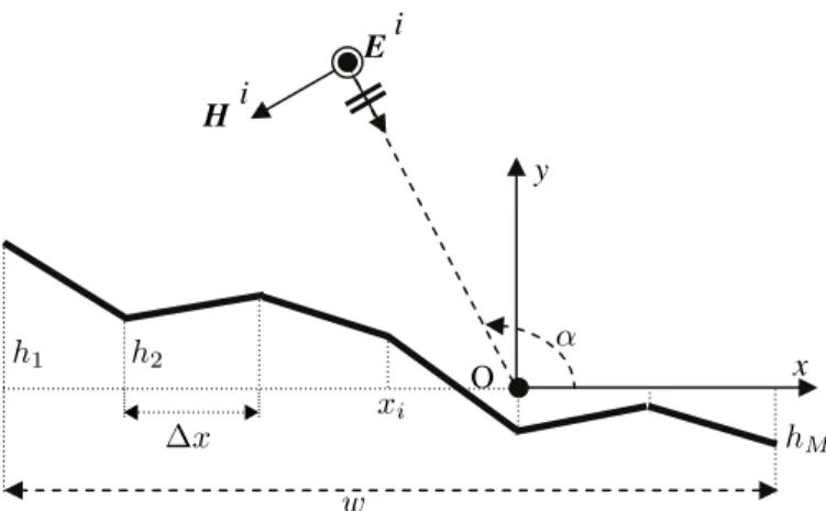
Fig. 1: Rough surface described by a set of correlated random variables (RVs)hi.

then the total number of independent RVs after KL transform stays as large as the number of correlated RVs, leading to a high-dimensional problem. In [6], where a finite element method (FEM) was adopted, this was dealt with by dividing the space of variables into subspaces with a correlation length comparable to their size. Nevertheless, when using an integral equation (IE) formulation, where the electromagnetic behavior is described globally, such an approach as described in [6] is not possible. Therefore, in this letter, we introduce another transformation to tackle the correlation, i.e. the Cholesky transformation. This alleviates the curse of dimensionality within the IE-based SGM-MLFMM framework.

This letter is organized as follows. Section II describes the the-oretical framework of the stochastic MLFMM with correlated RVs. An illustrative numerical example of the scattering at a two-dimensional (2D) rough surface is given in Section III. Section IV concludes the letter.

II. CHOLESKY-BASEDSGM-MLFMM

As a generic example for full-wave stochastic problems with correlated RVs, in this letter, we consider two-dimensional frequency domain scattering from a perfect electrically con-ducting (PEC) plate of width w, residing in free space. As depicted in Fig. 1, the plate’s roughness is stochastically defined by letting the height ofM nodes, equidistantly spaced along thex-axis, vary randomly. These heights are described by a set of M correlated Gaussian variables, collected in

M], and with correlation matrix Σ.

The elements of the correlation matrix are given by: Σij = σ2exp (−|xi− xj|

2

L2 c

), i, j = 1, ..., M, (1) where σ is the standard deviation and Lc the correlation

length. Traditionally, in order to apply PCE, the correlated RVs are converted into independent RVs, collected in vector ξ= [ξ1, ξ2, ..., ξR] via the KL transform as follows:

h= µ + U Λ1/2ξ, (2)

where µ is the mean value of h, and U and Λ are matrices defined by the eigenvalue decomposition of the correlation matrix Σ, i.e.

Σ = U Λ UT. (3)

Note that the number of independent parameters R may be smaller than the number of correlated parameters M (R 6 M ). The standard electric field IE description of the scattering problem of Fig. 1 in conjunction with the Method of Moments (MoM) yields a linear system that is dependent on ξ [4]:

Z(ξ)I(ξ) = V (ξ), (4)

with Z(ξ) the MoM system matrix, I(ξ) the vector collecting the unknown current densities and V(ξ) the known RHS. All quantities in (4) are expressed in PCE form, e.g. for Z(ξ):

Z(ξ) =

K

X

k=0

Zkφk(ξ), (5)

where{φk(ξ)}k=0,...,K represents a set ofK + 1 mutually

or-thonormal multivariate polynomials according to the Wiener-Askey scheme. In the case of Gaussian variables h (and thus ξ), these are products of univariate Hermite polynomials, dependent on a single RVξi. The total number of polynomials

grows rapidly withR as

K + 1 = (R + P )!

R!P ! , (6)

whereP is the total order of the polynomials φk(ξ), calculated

as the sum of the orders of the univariate polynomials they are composed of. Calculation of the PCE coefficients Zk is done

via projection, necessitating a multidimensional integration in the R-dimensional space of ξ:

Zk=< Z(ξ), φk(ξ) >= Z ξ1 ... Z ξR Z(ξ) φk(ξ) W (ξ)dξ1...dξR, (7)

where W (ξ) represents the multivariate Gaussian probability density function (PDF) of ξ. In particular, when the correlation lengthLcis low, the KL transform may lead to a dense, square

matrix UΛ1/2, i.e. R = M and each correlated RV hi is

dependent on all RVs ξ. Moreover, each matrix element of Z(ξ) will also depend on all RVs ξ, and the multidimensional integrals of type (7) become cumbersome to compute. After calculating the coefficients Vk in a similar way, solution

k

via Galerkin projection:

Vm= K X k,l=0 γklm6=0 Zk Il γklm, m = 0, .., K, (8)

whereγklm represents a three-term inner product of Hermite

polynomials:

γklm=< φk(ξ) φl(ξ), φm(ξ) > . (9)

Note that (8) constitutes a deterministic linear system with a complexity that scales with the number of non-zero numbers γklm, which follows anO(K1.5) law.

To expedite the solution of the linear system, MLFMM [7] is invoked, by dividing the structure into groups of sources. If the distance between a source and an observation group is large enough, then the system (4) can be approximated as:

D(ξ) T A(ξ) I(ξ) ≈ Z(ξ), (10)

where D(ξ), T and A(ξ) represent the well-known dis-sagregation, translation and aggregation matrix respectively. However, in contrast to the problems described in [3], whereas the aggregation and disaggregation matrices were dependent only on a group of sources, and thus only on few hi, here,

they are still dependent on all independent RVs ξ. Besides the aforementioned curse of dimensionality in calculating PCE projections (7), this also entails an unacceptably long solution time of (8). Indeed, since the aggregation and the disaggregation matrices are dependent on all independent RVs, their PCE coefficients are all nonzero and the complexity does not scale linearly with the number of polynomialsK as in [3], but with the total number of γklm.

To tackle this issue, instead of using the traditional KL transform, we propose to adopt a Cholesky transformation. Then, the correlated RVs are expressed via another vector of independent RVs η:

h= µ + L η, (11)

where L is a lower triangular matrix related to the correlation matrix as follows [8]:

Σ = L LT. (12)

To show the benefits of this Cholesky decomposition, for a canonical structure as shown in Fig. 1, with M = 200,

Lc = λ/5, σ = λ/20 and w = 20λ (with λ the

free-space wavelength), we present the structure of this particular correlation matrix in Fig. 2 and its corresponding KL and Cholesky matrices in Fig. 3. Whereas the KL matrix U Λ1/2 is a densely filled matrix, the off-diagonal elements of the Cholesky matrix L rapidly vanish as can be seen from Fig. 3. As of yet, a formal proof of this behaviour is still missing.

Consequently, when dimensionality reduction with KL transform is not possible, the benefits of the advocated Cholesky approach are:

• The M correlated RVs h depend only on a few

1536-1225 (c) 2016 IEEE. Personal use is permitted, but republication/redistribution requires IEEE permission. See http://www.ieee.org/publications_standards/publications/rights/index.html for more information. This article has been accepted for publication in a future issue of this journal, but has not been fully edited. Content may change prior to final publication. Citation information: DOI 10.1109/LAWP.2016.2603232, IEEE

Antennas and Wireless Propagation Letters

3 1 200 1 200 -16 -14 -12 -10 -8 -6 -4 -2 0

Fig. 2: Magnitude (on a logarithmic scale) of the elements of the correlation matrix Σ for a canonical problem.

1 200 1 200 -6.5 -6 -5.5 -5 -4.5 -4 -3.5 -3 -2.5 -2 -1.5 (a) KL matrix 1 200 1 200 -16 -14 -12 -10 -8 -6 -4 -2 0 (b) Cholesky matrix

Fig. 3: Magnitude (on a logarithmic scale) of the elements the matrices pertaining to the decomposition of Σ, shown in Fig. 2.

type (7) depending on these correlated RVs, are reduced in dimension, and their computation is expedited

• Many PCE coefficients are zero, as their corresponding

stochastic quantities, in particluar the elements of Z(η), only depend on a few independent RVs. This substantially improves the computational and memory complexity.

III. NUMERICAL EXAMPLE:

We consider scattering from a rough PEC strip of width w = 100λ, whose roughness is described by 81 RVs that determine the y-coordinates of the equally distributed points on the structure, as presented in Fig. 1. The correlation length is Lc = λ and the standard deviation is σ = λ/20.

The incident field is a TM-polarized plane wave impinging under an angle of α = 3π/4. The structure is discretized with N = 2 000 segments and the unknown current density

0 50λ 100λ 3 4 5 6 |E [Js ]| [mA/m] SGM MC

Fig. 4: Average current density E[Js] on the rough strip, with

E[·] the expectation operator.

is defined adopting piecewise constant basis functions. All computations are carried out on a Dell PC with a quad-core Intel(R) Core(TM) i7-2600 processor operating at 3.40 GHz and with 8 GB RAM memory.

To validate the accuracy and demonstrate the efficiency of our novel method, a standard MC analysis with10 000 samples is used as a reference solution. This MC analysis takes about 7h. Moreover, the stochastic scattering problem is also solved by means of the non-intrusive PCE-based Stochastic Collocation Method (SCM) leveraging sparse Smolyak integration [9]. The results for the average current density with the SGM-MLFMM scheme and polynomial order2 leads to an accuracy of 0.15% compared to MC. The accuracy of SGM-MLFMM cannot be readily predicted on beforehand, but it can be increased by increasing the polynomial order. Also, SCM uses P = 2 and 13 285 Smolyak integration points. The timing analysis is as follows: the novel SGM-MLFMM scheme takes about 1h and SCM takes around 10h. The gain is achieved in both the setup and the solution phase, as visible from Table 1. If the KL transform would be used in combination with SGM, then the setup time for calculation of the PCE coefficients of D and A coefficients would be determined by (7), and would be of the same order of magnitude as the setup time of SCM.

TABLE I: Setup and solution time

method setup solution

SGM 99 s 3 948_s

SCM 26 570_s 7 971_s

MC 19 200_s 5 887_s

The average current density on the strip is given in Fig. 4 and its standard deviation is presented in Fig. 5. A good agreement between SGM and MC is visible. These results are presented for polynomial order P = 2 and the corresponding total number of stochastic unknowns Nstoc = (K + 1)N =

6 806 000.

To reduce possible truncation errors, as described in [3], the polynomial order should be chosen large enough such that the PCE of Z can be found accurately through multiplication and Galerkin projection of the PCE coefficients of D and A. To demonstrate the influence of the truncation error on the average

0 50λ 100λ 0.6 0.8 1 1.2 1.4 σ [Js ] [mA/m] SGM MC

Fig. 5: Standard deviation of the current densityσ[Js] on the

rough strip, with σ[Js] =pE[(Js− E[Js])(Js− E[Js])H].

45λ 50λ 55λ 3.68 3.7 3.72 3.74 3.76 |E [Js ]| [mA/m] P = 0 P = 1 P = 2

Fig. 6: Average current density in the middle of the rough strip for several polynomial orders.

current density, in Fig. 6 we present E[Js] in the middle

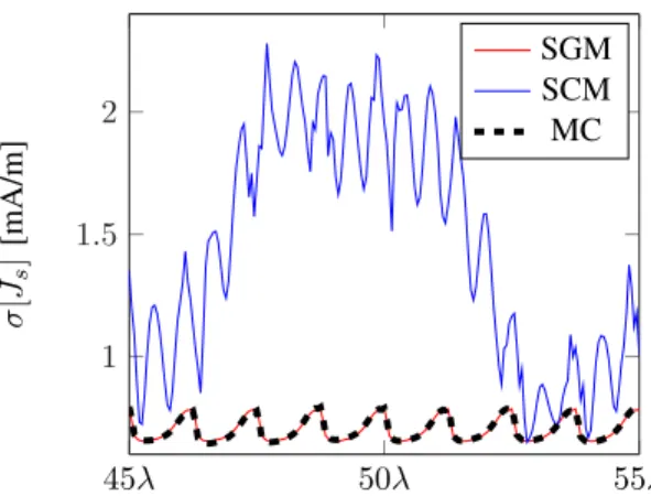
of the strip for several polynomial orders. From this figure, the convergence of the advocated SGM-MLFMM scheme is clearly visible, which also again validates our method. Moreover, at this point, it is important to point out that, in particular when dealing with full-wave problems, variations of the output parameters, such as current density, can be substantial and the Smolyak integration rule used in SCM may fail to produce good results. This is visible from Fig. 7, where the standard deviation of the current density Js in the middle

of the rough strip is shown. This behavior is well known for integration of functions that are not smooth enough [10]. The proposed SGM-MLFMM does not suffer from this issue, however, since the integration was done in a lower dimensional space thanks to the advocated Cholesky transformation. To achieve the same level of accuracy for the standard deviation, with the SGM, the number of Smolyak integration points should be increased to 722 089, which becomes prohibitively expensive. This clearly demonstrates the huge advantage the novel SGM-MLFMM scheme over SCM.

IV. CONCLUSION

In this letter, the UQ of full-wave stochastic problems, described by correlated RVs, was investigated. Classically, the KL transformation is applied to decorrelate the RVs.

45λ 50λ 55λ 1 1.5 2 σ [Js ] [mA/m] SGM SCM MC

Fig. 7: Standard deviation of the current density Js in the

middle of the rough strip.

However, for the envisaged applications, the SGM-MLFMM scheme, presented in literature before by the authors, can-not be straightforwardly extended by incorporating a KL transformation, and this because of two reasons: (i) the computation of the PCE coefficients entails integration in a highly-dimensional space; (ii) all these PCE are nonzero, as the stochastic quantities are dependent on all independent RVs after KL transformation. We proposed to tackle these issues by invoking Cholesky decomposition of the correlation matrix instead, leading to a very accurate and efficient SGM-MLFMM algorithm. The novel method was validated and compared against a MC analysis and a SCM for the case of scattering at rough PEC plate.

REFERENCES

[1] T. El-Moselhy and L. Daniel, “Variation-aware stochastic extraction with large parameter dimensionality: Review and comparison of state of the art intrusive and non-intrusive technique,” in 2011 12th International Symposium on Quality Electronic Design (ISQED 2011), 14-16 March 2011, Santa Clara, CA, USA, 2011, pp. 508–517.

[2] C. Chauvi`ere, J. S. Hesthaven, and L. C. Wilcox, “Efficient computation of RCS from scatterers of uncertain shapes,” IEEE Transactions on Antennas and Propagation, vol. 55, no. 5, pp. 1437–1448, May 2007. [3] Z. Zubac, D. De Zutter, and D. Vande Ginste, “Scattering from

two-dimensional objects of varying shape combining the Multilevel Fast Multipole Method (MLFMM) with the Stochastic Galerkin Method (SGM),” IEEE Antennas and Wireless Propagation Letters, vol. 13, pp. 1275–1278, 2014.

[4] Z. Zubac, J. Fostier, D. De Zutter, and D. Vande Ginste, “Efficient uncertainty quantification of large two-dimensional optical systems with a parallelized Stochastic Galerkin Method,” Opt. Express, vol. 23, no. 24, pp. 30 833–30 850, Nov 2015.

[5] M. Loeve, Probability Theory II. Springer, 1994.

[6] Y. Chen, J. Jakeman, C. Gittelson, and D. Xiu, “Local polynomial chaos expansion for linear differential equations with high dimensional random inputs,” SIAM Journal on Scientific Computing, vol. 37, no. 1, pp. A79– A102, 2015.

[7] W. C. Chew, J. M. Jin, E. Michielssen, and J. Song, Fast and Efficient Algorithms in Computational Electromagnetics. Norwood, MA: Artech House, 2001.

[8] N. J. Higham, “Cholesky factorization,” WIREs Comp. Stat., vol. 1, no. 2, pp. 251–254, 2009.

[9] Z. Zubac, D. De Zutter, and D. Vande Ginste, “Scattering from two-dimensional objects of varying shape combining the method of moments with the Stochastic Galerkin Method,” IEEE Transactions on Antennas and Propagation, vol. 62, no. 9, pp. 4852–4856, Sep 2014.

[10] P. Tsuji, D. Xiu, and L. Ying, “Fast method for high-frequency acoustic scattering from random scatterers,” International Journal for Uncertainty Quantification, vol. 1, no. 2, pp. 99–117, 2011.