Duclos: Professor, Département d’économique, Université Laval and CIRPÉE [email protected]
Fortin: Professor, Département d’économique, Université Laval, CIRPÉE, CIRANO and holder of Canada research Chair in Economics of Social Policies and Human Resources
[email protected] Fournier: Analysis Group, Inc.
This work was made possible thanks to the cooperation of the Ministère de l’emploi et de la solidarité sociale du Québec, where the microsimulation model that enabled us to initiate this project on effective marginal tax rates in Quebec was developed. We wish to specifically thank Marco de Nicolini and François Godin for their assistance, as well as the SSHRC and the FQRSC for their financial support. This paper is an extension of Duclos, Fortin and Fournier (forthcoming).
Cahier de recherche/Working Paper 07-46
An Analysis of Effective Marginal Tax Rates in Quebec
Jean-Yves Duclos Bernard Fortin
Andrée-Anne Fournier
Résumé:
Cet article dresse un portrait de la situation des taux marginaux effectifs d’imposition (TMEI) sur le revenu de travail au Québec. Il vise à permettre une meilleure compréhension de l’impact des politiques gouvernementales sur le comportement des agents économiques. À l’aide d’un modèle de microsimulation comptable reproduisant les systèmes d’impôts et de transferts au Québec pour 2002, nous mesurons les TMEI qui résultent de l’interaction des mécanismes de perception et de redistribution. En outre, nous en évaluons la répartition au sein de la population. L’analyse de ces taux démontre, entre autres, que la politique familiale du gouvernement, dont l’aide est ciblée vers les familles à faible revenu, engendre des TMEI élevés attribuables à la réduction généralement rapide des transferts avec le revenu de travail. Ainsi, plus du quart des chefs de famille monoparentale ont un TMEI pouvant atteindre, et même excéder, 80 %. Quant aux familles biparentales, elles font majoritairement face à un TMEI qui approche 50%. Nous montrons l’importance de tenir compte de l’hétérogénéité, à la fois selon les types de familles et selon les niveaux de revenu, de manière à bien évaluer la variabilité des TMEI à travers la population.
Mots Clés: Taux d’imposition, fiscalité, microsimulation, politique familiale
Abstract :
This article draws up a portrait of effective marginal tax rates (EMTRs) on labour income in Quebec. It aims at allowing a better understanding of the impact of tax policy on the behavior of economic agents. Using an accounting microsimulation model that reproduces the system of taxes and transfers in 2002 Quebec, we measure the EMTRs that result from the interaction of the mechanisms of income taxation and redistribution. Moreover, we evaluate the distribution of EMTRs in the population. The analysis of EMTRs shows, inter alia, that family policy, whose assistance is targeted towards low-income families, generates high levels of EMTRs ascribable to the generally fast reduction of transfers as income increases. More than a quarter of heads of single-parent households face an EMTR which can reach, and even exceed, 80%. As for the two-parent families, they mostly face EMTRs of around 50%. We show the importance of accounting for EMTR heterogeneity, both with respect of types of families and levels of incomes, as well as evaluating the variability of EMTRs in the population.
Key words : Effective tax rates, taxation, microsimulation, family policy JEL codes : D31, D63, H21, H24, I38
1. Introduction
Implementation of redistributive policies by the government generally gives rise to the familiar trade-off between efficiency and equity. We say of a tax system that it is efficient when it minimizes the distortions in the behaviour of economic agents for any level of tax revenues. The tax rates implied by a tax system - while necessary to finance wealth redistribution programs designed to increase equity - may indeed create non-negligible inefficiency costs by modifying the environment within which individuals make decisions. Furthermore, the social transfer system introduces tax rates (albeit implicit) to the extent that the level of the transfers falls with increases in individuals’ income. In this context, the design of efficient government policies, as well as the analysis of their impact, requires a thorough understanding of the interaction of tax and transfer systems.
This provides the main justification for this article. Its main contribution is to present the results of a simulation model that reproduces the system of taxes and transfers in Quebec so as to better understand the impact of fiscal mechanisms and income support programs on incentives to earn labour income. The simulation model indeed allows a detailed descriptive analysis of effective marginal tax rates (EMTRs) on personal and household income as they result from tax collection and redistribution. These rates depend in a complex and nonlinear fashion on the characteristics of individuals and households as well as on the level and their type of income. We use our model to estimate these EMTRs and describe their distribution and composition within the population of Quebec. We characterize households for which the family structure and the income composition is such that financial incentives are very weak at the margin - in some cases even nil or negative. Within this exercise we pay particular attention to the situation of families with children since these are, a priori, most affected by the complexity of Quebec’s tax collection and income redistribution mechanisms.
A recent publication by the OECD, which dealt extensively with the issue of EMTRs, underscores the importance of a thorough understanding of fiscal mechanisms, such as the one our examination of Quebec allows:
The analysis of how benefits and taxes depend on work status and earnings levels does not, by itself, tell us how changes in tax-benefit policy will actually influence labour supply or how many individuals live in income poverty and why. It does, however, contribute to a thorough understanding of the mechanics of benefit systems. This understanding of how different tax-benefit instruments interact with each other, as well as with people’s particular labour market and household situations, is an essential pre-requisite for identifying tax-benefit reform priorities [OCDE (2004)].
The originality of our work is that of drawing a rich and original portrait of the distribution of marginal rates throughout the population of Quebec. To the best of our knowledge, only a single Canadian study, that of Macnaughton et al. (1998), has allowed these effective rates and their distribution across the population to be estimated. This latter study does not cover, however, all of the transfer programs we modelled in Quebec, in particular social assistance.
and discusses its implications for computing the marginal cost of public funds. It also presents a qualitative analysis of the impact of family policy, as it has recently been implemented in Canada and Quebec, on EMTRs. Section 3 is devoted to presenting the model and the data used. Section 4 discusses all the results. Here we look at various measures of the joint distribution of EMTRs and the incomes and characteristics of households. We also decompose the mean rates so as to better understand the impact of different measures of taxation and transfer payments. Section 5 concludes.
2. Effective marginal tax rates 2.1 Definition
In a document published by the Commission parlementaire sur la réduction de l’impôt des particuliers1 in 1999, EMTRs2 are described as a phenomenon that arises out of two
mechanisms, collecting personal income taxes while simultaneously maintaining a policy of income support. Transfer programs are established in order to provide additional income to some citizens. They can take the form of direct social transfers or of tax code provisions that reduce the tax burden (or yield a rebate). The progressive nature of our tax system, combined with the selectivity of transfer programs, means that an increase in household income results in a double jeapordy: transfers are cut at the same time as taxes rise. As a third element, we add payroll taxes3.
Mathematically, an EMTR is defined as follows. Assume, to simplify, a one-adult household. Let his disposable income be defined with the identity:
, YD=YL YO T+ − +TR ; transfers social ; ) deductions payroll (including taxes sales and income ; income labour -non private, ; income labour ; income disposable where = = = = = TR T YO YL YD (2.1)
with T =T(YL,YO,Z) and TR=TR(YL,YO,Z), and where Z is a vector of individual
characteristics. Thus, we have: ( , , ) ( , , ) YD=YL YO T YL YO Z+ − +TR YL YO Z . (2.2)
1 The Commission parlementaire sur la réduction de l’impôt des particuliers is not alone in its interest in the
issue of EMTRs. Indeed, it follows in the footsteps of several other commissions and studies that have examined this phenomenon, such as the White Paper on the Personal Tax and Transfer Systems (1984), the Commission sur la réforme de la sécurité du revenu (1996), and the Commission sur la fiscalité et le financement des services publics (1996).
2 The Government of Quebec uses the term “implicit” rather than “effective.” We, however, prefer to reserve
the expression “implicit rate” for transfer programs and use “effective rate” to capture income taxes and transfers. Thus, we primarily refer to “effective rates” in this text.
3 We assume in this analysis that payroll deductions paid by the employee are perceived as taxes, and not as a
source of future income (e.g., QPP premiums) or as an insurance premium for guarding against a risk such as the future loss of employment (e.g. , Employment Insurance premiums).
Differentiating with respect to YL (to simplify, we assume that T(.) and TR(.) are differentiable in YL) yields:
( ) ( ) 1 . (2.3) dYD T TR dYL YL YL ∂ ⋅ ∂ ⋅ ⎡ ⎤ = −⎢ − ⎥ ∂ ∂ ⎣ ⎦
Using equation (2.3), we define the EMTR on labour income as follows: ( ) ( ) 1 dYD T TR EMTR dYL YL YL ∂ ⋅ ∂ ⋅ = − = − ∂ ∂ . (2.4)
The r.h.s. of Equation (2.4) reveals that the EMTR is the product of increases in income and sales taxes combined with decreases in transfers (when applicable) resulting from a marginal rise in income YL. The EMTR thus includes an explicit and an “implicit” component. The latter (also called the clawback rate) is defined as the proportion of the amount of transfers forfeited subsequent to a marginal increase in labour income.
2.2 Distortions and the marginal cost of public funds
The EMTRs under investigation create a gap at the margin between the social and private profitability of individuals’ behaviour on the labour market. Thus, they are at the root of distortions in many decisions, such as labour market participation, the number of hours worked, the level of work effort, investments in human capital (education, professional training, etc.), the geographical mobility of labour, occupational choices, and black-market labour.
The presence of EMTRs also modifies the calculation of the marginal cost of public funds (MCPF), i.e., the cost to society of a one-dollar increase in tax revenues destined to fund public expenditures. In principle, this supplementary cost must be incorporated into any cost-benefit analysis of government programs. Browning (1976) observes that the social cost of financing a marginal dollar of public expenditures is the sum of that dollar, which can no longer be used for private purposes, plus the change in total costs and social welfare caused by the distortions in individual choices created by the increased EMTR imposed when collecting that dollar. This sum is the MCPF, which thus incorporates the direct tax burden as well as the supplementary bonus. It has been demonstrated (e.g,. Fortin and Lacroix, 1994) that, in a linear economy of identical individuals in which the individual’s only choice is between leisure and consuming a private good, in which taxes are collected from a proportional tax on income (at a rate
τ
), and in which the public good is separable in the individual’s utility function, we have:1 , 1 1 CMFP
τ η
τ
= − − (2.5)where η is the uncompensated elasticity of labour supply with respect to the net wage rate. Equation (2.5) reveals that the MCPF is increasing in the EMTR, at least to the extent that the uncompensated labour supply elasticity is positive. Thus, when η = 0.3 and
τ
= 0, the MCPF is 1 dollar, while it is $1.43 whenτ
=0.5. In this latter case, there is an additional cost (= $0.43) at the margin for society to finance one dollar in additional public expenditure, owing to the greater marginal distortion in the hours of work.More generally, distortions in the number of hours of labour supplied, as measured by the MCPF, depend on a combination of three factors: the level of effective rates of taxation on labour income, the distribution of individuals (or households) across these rates, and the sensitivity of individuals’ labour supply behaviour.4 In this article, it is the distribution of the values of
τ
that are of particular interest to us. As we have seen, the MCPF increases withτ
(assuming thatη
> 0), suggesting that the cost of financing public expenditures increases with their aggregate funding levels. However, it is not only the average level ofτ
confronting individuals that matters. It is, in fact, possible to demonstrate that the MCPF is convex inτ
. Thus, for a given mean ofτ
, the greater its variability across individuals, the greater society’s MCPF. Consequently, in this article we will closely examine the mean as well as the distribution across individuals of the EMTRs.2.3 The role of family policy
Family policy, especially when it is targeted at low- and medium-income households, has a particularly pronounced incidence on the level and variability of the EMTR. This policy comprises a series of fiscal measures and transfer programs designed to support family incomes. In Quebec, it involves both levels of government, provincial and federal. Here we will simply provide a brief description of the main modifications to family policy having been implemented during the 15 years preceding 2002,5 along with their anticipated
implications for the EMTR.
In 1993, the federal government abolished two measures with universal coverage, the family allowance and the child tax credit,6 in order to focus financial assistance on low
income families.7 These programs were replaced with the Canada Child Tax Benefit (CCTB),
which includes a supplement to labour income for low-income families on top of a basic transfer. In addition, the federal government opted to grant a GST tax credit which, like the CCTB, is intended to provide a fiscal incentive to work. In 1997, the Government of Quebec also undertook a thorough reform of the assistance given to children. The design of the family allowance has thus been re-examined. In the past, it was simply a universal program whose generosity increased with the number of children. Since the reform, the family allowance has become a package of financial assistance measures targeted exclusively at low-income families. Moreover, the weight of children in social assistance schedules (now called employment assistance) has become an element of the family allowance. Finally, a universal daycare system at $5 per day was established.
At the provincial level, a non-refundable tax credit is extended to taxpayers with
4 Dahlby (1998) derived an expression for the MCPF associated with a hike in the tax rate under a progressive
tax system that accounts for the distribution of individuals and the different rates they face. Essentially, this is a matter of capturing changes to government revenue from each tax bracket subsequent to a change to the marginal rate of one of the brackets. This can be done with our model.
5 A complete portrait of the history of the government’s participation in assistance to families is found in Rose
(2001) and Vincent and Woolley (2001).
6 The federal government continues to offer a non-refundable tax credit for the first child of a single-parent family. 7 This support generally provides a level of assistance (in the form of a benefit, an allowance, a credit, etc.) that
reaches its maximum for households whose family income varies between $20 000 and $30 000, approximately. As of a certain threshold located between two boundaries, the financial assistance paid out is gradually reduced until it reaches zero for medium- to high-income families.
dependent children. A supplement is added to the base amount in the case of single-parent families as well as for parents whose children are enrolled in postsecondary education. Taxpayers with dependent children are also eligible for a tax cut with respect to the family.8
Finally, the provincial government continues to provide financial assistance for daycare through the refundable tax credit for daycare expenses incurred by families unable to take advantage of the $5 per day service. The federal government, for its part, has opted for a tax deduction for daycare costs, deeming them to be expenses incurred for employment that reduce parents’ ability to pay income taxes.9
Overall, both levels of government have chosen to focus on vertical redistribution. This approach seeks to increase the contribution of wealthier families to assisting poorer families (Baril et al., 1997). Universality in assistance to families has thus almost completely disappeared, and higher and more variable EMTRs upon exiting from income support programs are the flipside of the highly targeted policies for which the federal and provincial governments have opted in recent years.
3. The model and the data used
3.1 Structure and assumptions of the model
The type of model we constructed to examine the distribution of EMTRs in Quebec simulates personal income taxes and governmental transfer programs for a sample of individuals, households, and families obtained from survey and administrative data (cf. Gupta and Kapur [2000] for a general presentation of these models). The model we use was initially created at the Ministère de l’emploi, de la solidarité sociale et de la famille du Québec (MESSF). We adapted it to our purposes. This is a static model that performs accounting calculations to reproduce taxes and transfers for the year 2002. On the basis of the information contained in the database, the simulations replicate the income declarations of each household in the sample and account for the various transfer programs to which it has access. A complete description of the measures applied by the governments of Quebec and Canada that are included in our model is provided in Appendix A.
Several assumptions are necessary for performing a full simulation of tax and transfer programs. For example, no information regarding the amounts of daycare costs incurred by households with children is included in the database. Consequently, this had to be estimated. Thus, we let all families benefit from the $5 per day daycare service.10 In reality, for a
number of reasons, not all parents benefit from this government program. Furthermore, we assume that only 50 per cent of the families eligible for the Parental Wage Assistance (PWA) program take advantage of it. It would not be realistic to include them all, since only families
8 This tax cut plays a different role than that of the non-refundable tax credit. The non-refundable tax credit is a
fiscal measure that benefits all families, i.e., it is not income contingent. The credit corresponds to 20 per cent of an amount that varies with the number of children. The principle of universality no longer obtains in the case of the tax reduction for families, since this measure essentially benefits low income families: the allowable tax deduction is reduced by 3 per cent of the family income exceeding $26,700.
9 Vincent and Woolley (2001) compare the two levels of government in terms of what is unique in each one’s
approach to the tax treatment of daycare expenditures.
10 It is also possible to run all simulations with regular daycare costs. The tax treatment in effect is then that
that apply obtain this form of income support. According to the MESSF, approximately 47 per cent of eligible families benefited from the program in 2002. A complete description of our various assumptions is included Appendix B.
3.2 Descriptive Statistics
In the literature, the descriptive analysis of EMTRs is based on two different approaches. Most authors resort to representative agents to compare effective taxation on different household categories. This method is widely used, in part because it is relatively easy to implement. The second approach consists of determining the distribution of EMTRs across the population. It allows a much more complete analysis, but also requires the use of a representative database of households. The model we use has the advantage of allowing results from both of these approaches to be generated.
One example of a representative tax profile is shown in Figure 1 for a two-parent family with one income, two children aged 3 and 5, and participating in the PWA program for the tax year 2002. For the calculations we assume a single source of labour income as well as successive $10 wage increments.
Figure 1 : Example of a tax profile (two-parent family)
Source: Direction de l’analyse économique et des projets gouvernementaux, MESSF
0 5 000 10 000 15 000 20 000 25 000 30 000 35 000 0 5 000 10 000 15 000 20 000 25 000 30 000 Total income ($) Di sp os ab le i n co m e ( $ ) -60% -40% -20% 0% 20% 40% 60% 80% 100% 120% 140% 160% 180% 200% EM TR
Figure 1 depicts the evolution of the EMTR as a function of the family’s labour income and reveals the zones in which the rates are highest. Quebec’s finance ministry also has its own model of disposable income, yielding the implicit marginal rates that are published in Commission sur la réduction des impôts des particuliers (1999) and that underlie the results presented in Ouellet (1998). An analysis of representative tax profiles is also used by Bernier and Lévesque (1995) and Laferrière (2001), who address the programs of the federal and provincial governments, as well as by Davies (1998), who deals exclusively with federal taxes and transfers. Recently, a study by the OECD (2004) also evoked this technique. This study was unique in presenting the budget constraints of different household types for some twenty countries, OECD members and non-members.11 Three important elements
11 Canada was not included in this study.
Revenu disponible Taux marginal d'imposit ionEMTR Disposable income
generally differentiate between studies having been conducted using representative agents: the number of different household types retained, the income intervals considered, and the set of fiscal measures and transfers incorporated into the study. An important finding emerges in most representative agent studies: it is those households that are net beneficiaries of government transfers that confront the highest EMTRs (Government of Quebec, 1999). More generally, it is those with low incomes that are most highly taxed (in effective terms) at the margin (Bernier and Lévesque, 1995; Ouellet, 1998; Davies, 1998; and Laferrière, 2001). This result is not surprising if we examine the structure of governmental transfer policies. In order to target assistance at the most needy households and curb the costs of government programs, transfer measures are indeed accompanied by very high clawback rates (i.e., the level of financial assistance declines very rapidly as family income rises), thus increasing the EMTR.
Nonetheless, there are limitations to the conclusions that can be drawn from an analysis of representative agents. A demonstration that a family with very specific characteristics has an extremely high EMTR within a certain income bracket tells us nothing about how many families are in that position. Therefore, Davies (1998) pushes the analysis a little further, calculating the mean effective rate facing Canadians (51 per cent in 1994). However, this result is based on aggregate data, thus limiting the level of precision of his work.
More detailed studies have been conducted to determine the distribution of EMTRs across the population and to describe the characteristics of individuals facing the highest rates. In 1998, a U.S. study by the Joint Committee on Taxation compared statutory rates (which only reflect the income taxation mechanism) and EMTRs for all households in the country. The study highlighted the fact that 25 per cent of U.S. taxpayers face an EMTR that differs from the official tax rate. In Canada, the corresponding value is 56 per cent12 for the
same fiscal year (Macnaughton et al., 1998). Work by Macnaughton et al. (1998) also revealed that high EMTRs are mostly found amongst taxpayers in the 17 per cent bracket, i.e. those whose incomes are lowest. While only 2 per cent of individuals whose income is in the highest tax bracket are confronted with a different EMTR than that explicitly provided for by the Act, 89 per cent of those taxed at 17 per cent are in that situation. The authors further mention that, aside from income, family characteristics have an impact on the EMTR. Among other things, the effective EMTR increases by two or three percentage points per child - an effect that disappears in the case of families in the highest income brackets. The study by Laroque and Salanié (1999) on the tax and transfer system in France yields results that parallel those generated by Canadian and U.S. simulations.
3.3 The data used
The data we use are from Statistics Canada’s Social Policy Simulation Database and Model (SPSD/M). This model was designed to permit the analysis of fiscal policy, transfer programs, and sales taxes for all Canada or for individual provinces. We extract data from
12 This is probably a lower bound, since social assistance, which is at issue in the high values of EMTRs, is not
this microsimulation model and perform calculations with our own model. We proceed in this way because the SPSD/M system is not flexible enough for our purposes and also because some Quebec policies, such as the PWA program, have not been incorporated into it. Nonetheless, we deem the SPSD/M database to best suited to our information needs. It was constructed by combining individual administrative data from personal tax returns and historical data on EI recipients with survey data on family incomes and expenditures.
Five main sources of data allowed the Social Policy Simulation Database (SPSD) to be constructed. The first is the Consumer Finance Survey, which is the principal source of information available to Statistics Canada regarding the distribution of income across individuals and families. Essential information for the simulations we conducted is found in it. A second source of information comes from individual tax returns. These returns provide important information that is complementary to survey data, but is severely handicapped by the absence of detailed information on several aspects of taxation. A sample of historical EI claims represents the third source of microdata. The fourth is the Household Expenditure Survey that is periodically conducted by Statistic Canada. In addition to containing very detailed data on Canadians’ incomes and the structure of household expenditures, its main contribution is to supply information on net changes to households’ assets and liabilities. Data on savings proved particularly useful during the simulations, for example to determine a family’s eligibility for the PWA program (a means test is imposed to determine whether a low-income family qualifies for the transfer). The developers of the SPSD drew on one final source, the Survey of Labour and Income Dynamics. This is a longitudinal survey of households that provides data on income and labour-market experience.13 The SPSD,
containing much more information than a single survey, has all the variables required for the simulations we wish to run.
The data we extracted from the SPSD were initially stored at the level of the individual. We aggregated individuals into a broader grouping, the census family, while retaining the information on each member (for example, labour income of the household head as well as of other family members). The SPSD defines a census family as “a head, their [sic] spouse (if there is one), and their children under the age of 25 (including their guardian children), living together in the same dwelling.” Thus, two single individuals living under the same roof constitute two census families. Consequently, in the context of our fiscal analysis, these two individuals are considered separately. We also treat an individual aged 18 and over, who is not studying and who earns a taxable income but still lives at home, as single. This processing of the initial database allows us to obtain a sample suitable for tax analysis.
4. Analysis of the results
Microeconometric studies having examined the impact of government policies on labour supply have generally concluded that the elasticity of labour supply with respect to the net wage rate is relatively low for the population as a whole. However, these elasticities can be greater for specific groups, such as the heads of single-parent families. As a consequence,
13 For more information regarding the micro databases and their creation, consult the SPSD/M document Database Creation Guide.
it is vital to go beyond the mean impacts that tax and transfer mechanisms might have to analyse their incidence in the framework of specific family situations, in particular at various income levels.
Our microsimulation model makes this possible by measuring EMTRs for a representative sample of the population. Using various tools, such as representative tax profiles and density graphs, we paint a picture of the situation of EMTRs in Quebec. We address the level, distribution, and composition of rates and describe the characteristics of households in the different effective tax brackets. Recall that, as we already mentioned in Section 2.2, the MCPF is convex with respect to the EMTR. Consequently, for a given mean EMTR, the MCPF increases with the variability of the EMTR, and it is thus important to account for this variability.
4.1 Representative tax profiles
As we underlined in Section 3.2, recourse to representative tax profiles is a relatively easy way to compare effective taxation between various household categories. Our presentation differs from that based on representative agents that we generally find in the literature because it is associated with a total EMTR that allows the contribution of each element of the tax and transfer system (income taxes, tax credits, tax rebates, programs to assist families, income supplements, employee payroll taxes such as QPP and EI) to be illustrated. Three tax profiles will be the subject of a brief presentation. For each one, the EMTRs (computed using $10 increments14) are presented for family incomes varying
between 0 and $70 000.15 We opted for a $10 increase, at the margin, in order to illustrate
more clearly the discontinuities associated with entry and exit thresholds for the various social programs. Furthermore, sensitivity analysis conducted on increments ranging from $10 to $1000 reveals that the evolution of the marginal rate in the framework of an analysis of representative tax profiles changes little as a function of the retained income level.
4.1.1 Single individuals
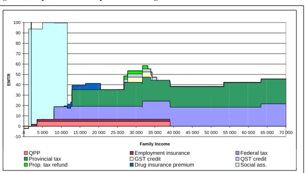
The tax profile of a representative single person is illustrated in Figure 2. Its presentation is relatively straightforward, owing to the limited number of fiscal measures and programs affecting this type of household. We note that the EMTR is initially negative, i.e., the amount received in transfer payments rises following an increase in income. This is because social assistance (also called employment assistance in Quebec) is not affected by the first dollars earned, while the GST credit rises with income. When income exceeds a penalty exemption threshold ($1200 when the individual is not affected by employment constraints), the presence of social assistance, in conjunction with QPP and EI premiums, pushes the EMTR over 100 per cent. Only when income approaches $12 000 does the single individual experience a decline in the EMTR. In this situation the concept of a “poverty trap”
14 The increase in household income is attributable to a wage raise given to the individual who is considered the
“household head” according to Statistics Canada’s classifications.
15 When the family income exceeds $70 000, the effective marginal tax rate stabilizes at about 45 per cent
(depending on the characteristics of the household). With a few exceptions, only fiscal measures on income taxes are imposed on the dollar earned at the margins, while transfer programs generally have no impact on higher income brackets.
truly comes into its own, since we can graphically visualize the presence of a barrier that impedes any incentive to work on behalf of social assistance recipients. Let us also underline the presence of a discontinuity in the rate when income reaches a level that triggers EI premiums (this premium, at 2.20 per cent, applies to the first $2000 earned in excess of this employment income threshold). Finally, we observe that these calculations omit some special benefits accruing to certain social assistance recipients (e.g., the drug insurance plan, dental care, disaster relief, etc.) that are terminated when they are no longer in the program. In this case, the EMTR can easily exceed 100 per cent.
Figure 2 : Representative tax profile for a single individual
-10 0 10 20 30 40 50 60 70 80 90 100 0 5 000 10 000 15 000 20 000 25 000 30 000 35 000 40 000 45 000 50 000 55 000 60 000 65 000 70 000 Family Income EM T R
QPP Employment insurance Federal tax
Provincial tax GST credit QST credit
Prop. tax refund Drug insurance premium Social ass.
Let us now observe the evolution of the EMTR after leaving social assistance. The conjunction of federal and provincial income taxes, premiums (QPP, EI, and the drug insurance plan), credits (GST and Quebec Sales Tax, QST), and property tax refunds causes the EMTR to vary between 35 and 58 per cent. Aside from the previously mentioned elements, an individual living alone receives an income tax credit. In the graphical representation reproduced above, this credit is included in the category “provincial income tax.” Above $26 700, the reduction in the credit results in an increase in 3.1 per cent in the marginal rate attributable to provincial income tax. When single individuals earn over $70 000, their EMTRs stabilize at 45.7 per cent, then at 48.2 per cent at $103 000.
4.1.2 The single-parent family
Overall, the EMTR of the single-parent family is higher and more variable than that of the single individual, owing to its eligibility to a greater number of transfer programs. One example is the National Child Benefit Supplement offered by the Government of Canada, with a rate reduction of 32.1 per cent for families with three children. Figure 3 illustrates the tax profile of the single-parent family.
As is the case for single individuals, we point out that the EMTR can be negative for very low income families. This situation is possible because of the PWA program.16 Figure 3
illustrates how the PWA program cuts the EMTR, as the hatched section represents the progression of the rates in its absence. Thus, we see that this government measure partially “breaches” the barrier formed by the reduced social assistance benefits following from a rise in income. Comparable results are obtained from the analysis of representative agents conducted by Bernier and Lévesque (1995), as well as from the Commission parlementaire sur la réduction de l’impôt des particuliers (1999). Conversely, once the single-parent family leaves social assistance, the PWA benefit, along with its supplement (which subsidizes fees for daycare services), are gradually reduced, triggering an increase in the EMTR that may reach 154.6 per cent17 at the $15 000 to $18 000 level.
Note that the rate is relatively low between $23 000 and $25 000, an income level as of which transfers and credits begin to decline, bringing the EMTR to 80 per cent for the single-parent family (with an income between $28 000 and $36 000, approximately). Notice that the category “provincial income tax” includes the income tax abatement for families. As it is cut (following the increase in income), the marginal rate attributable to provincial income taxes rises by 3 per cent. Also note the presence of high clawback rates, especially for family allowances (35 per cent between $15 340 and $21 200), the CCTB (22.5 per cent between $25 150 and $35 700), and the PWA program with its supplement (43 per cent between $15 340 and $18 460). As of $70 000, the EMTR of single-parent families stabilizes at approximately 50 per cent.
Figure 3 : Representative tax profile for a single-parent family
-20 0 20 40 60 80 100 120 140 160 0 5 000 10 000 15 000 20 000 25 000 30 000 35 000 40 000 45 000 50 000 55 000 60 000 65 000 70 000 Family Income EM T R
EI QPP Federal tax Prov. tax
GST credit CCTB Drug insur. premium PWA suppl.
Suppl. child Social ass. PWA QST credit
Family allow. Prop. tax refund Daycare Housing allow.
4.1.3 The two-parent family
Figure 4 illustrates the representative tax profile for a family consisting of two children and two adults with a single source of employment income. Note the absence of than the threshold below which social assistance benefits begin to decline for the single-parent family ($2400). Consequently, an income supplement is dispensed without the social assistance transfer being affected, which explains why the rate moves below zero before rising.
17 This rate is reached when we consider the rise in childcare fees confronting the heads of single-parent families
daycare costs and the PWA program supplement, since we assume that one of the two parents remains at home. As we pointed out in the case of the single-parent family, the hatched area represents the rates that would obtain in the absence of the PWA program. We observe that the taxation rate attributable to this program becomes positive (i.e., the amount of the benefit decreases) while social assistance is still received, bringing the marginal rate to over 100 per cent between $12 500 and $16 000 (this situation was also observed in the case of the single-parent family). Thus, the PWA program, which is supposed to provide an incentive to participating in the labour market, only partially achieves this goal. We note that the clawback rate (up to 43 per cent) contributes to maintaining the EMTR at over 60 per cent, even when the household ceases to be a net beneficiary of social assistance. Finally, we note that combining it with the Shelter Allowance program brings the total rate to more than 80 per cent for a family whose income is approximately $20 000.
Figure 4 : Representative tax profile for a two-parent family
0 20 40 60 80 100 120 0 5000 10000 15000 20000 25000 30000 35000 40000 45000 50000 55000 60000 65000 70000 Family Income E ff e ct ive m ar g in al r a te
EI QPP Federal tax Prov. tax GST credit
CCTB Social ass. Drug insur. premium QTS credit Family allow. PWA Prop. Tax refund Housing allow.
EI
Despite the fact that tax profiles provide a relevant illustration of the evolution of the EMTR, it must be borne in mind that they are only valid for the specific cases that were simulated. Since households are heterogeneous, a representative tax profile cannot be generalized to represent effective taxation of an entire population. Only application of the system of income taxes and transfers to a representative sample of a population can allow the distribution of the EMTR across that population to be examined.
4.2 Simulation from a sample
Table 1 presents the distribution of the four household types studied after the sample has been weighted. According to our sample, 2.9 million households are childless and slightly over 850 000 have children.
Table 1: Distribution of households by family status Number of households Proportion of total population Childless households 2 899 201 77% Single 1 830 259 49% Childless couple 1 068 942 28%
Households with children(s) 854 594 23%
Single parent 148 719 4% Two-parent family 705 875 19% All households 3 753 795 100%
Figure 5 : Distribution of households by family income
It is of some use to briefly examine the distribution of households by family income. Figure 5 illustrates this distribution for each of the four groups. The proportion of low-income households is higher among single individuals (61.2 per cent earning between $0 and $20 000) and single-parent families (51.1 per cent earning between $0 and $20 000) than among households with two adults. The group of two-parent families contains the highest proportion of households whose incomes exceed $40 000, 73.3 per cent (54.7 per cent for childless couples, 24.4 per cent for single-parent families, and 15.3 per cent for singles). Figure 5 also shows mean incomes, by parent and for the entire household - again, by family status. In Quebec’s fiscal system, income taxes are assessed on an individual basis that partially accounts for the income of the family to which the person belongs. Since we shall pay particular attention to examining EMTRs for families, we note that a gap of a little more than $25 000 separates the mean income of the head of a two-parent family from that of a single-parent family. This gap will have a significant impact on the distribution of the
51,1% 18,3% 9,1% 23,5% 24,6% 27,0% 17,6% 10,1% 16,3% 19,6% 22,8% 6,4% 15,3% 20,6% 19,8% 29,9% 61,2% 3,4% 1,8% 1,7% 0% 10% 20% 30% 40% 50% 60% 70% 80% 90% 100%
Single Single Parent Childless couple Two-parent f amily
80 000% and more 60 000 - 80 000$ 40 000 - 60 000$ 20 000 - 40 000$ 0 - 20 000$
Average income parent 1 : Average income parent 2 : A ver ag e f ami ly inco me :
20 792 $ 23 351 $ 37 148 $ 49 088 $
- - 16 742 $ 21 204 $
20 792 $ 23 351 $ 53 890 $ 70 292 $
EMTRs facing these families.
4.2.1 The distribution of the EMTRs
Using our model, we measure EMTRs for $1000 increments in household incomes.18
Various density measures were invoked to examine their distribution throughout the population. These allow us, for example, to determine the percentage of the population facing an EMTR that exceeds 60 per cent, or to characterize households for whom we find the highest effective rates. To do this we used nonparametric kernel estimation techniques (Fournier, 2005).
4.2.1.1 Marginal rates for the entire population: three peaks
Figure 6 presents the distribution of the population according to the values that the EMTR can assume. Three peaks characterize this distribution: zero EMTR, the 35 to 50 per cent tax bracket, and effective taxation at 100 per cent. With regards to the first peak, we first observe that 11 per cent of households benefit from a negative EMTR, i.e., marginal increase in their income will yield an additional net transfer. If we include, in this first group, all households for whom the effective rate of taxation is below 20 per cent, then one household in five benefits from a negative or relatively low rate.
Figure 6 : Density of the EMTR for the entire population
0 0,005 0,01 0,015 0,02 0,025 0,03 0,035 0,04 -20 -10 0 10 20 30 40 50 60 70 80 90 100 110 1
Marginal effective tax rate
De n s it y 10,6 % 8,9 % 27,8 % 38,9 % 3,9 % 5,1 %
The percentages listed between the arrows indicate the proportion of people in each area. Example: for 3.9% of households, the marginal effective tax rate is between 60 and 80%.
For nearly half of households (46 per cent), the EMTR falls between 35 and 50 per cent. For this second peak, in the centre of the graph, we distinguish between two sub-peaks, at 39 and 45 per cent. These two effective rates essentially correspond to the marginal rate of
18 The representative tax profiles we presented previously were based on a $10 increase, at the margin, in order
to illustrate more clearly the cuts associated with entry and exit thresholds for the various social programs. In order to analyse EMTRs across the population, we opted for a greater increase that probably better captures the situation of an individual receiving a wage raise. Furthermore, the $1000 raise is commonly used in the literature, especially by the Commission parlementaire sur la réduction de l’impôt des particuliers (1999) and by Laferrière (2001), making it easier to compare results. As for the representative tax profiles, the increase in household income is attributable to a wage raise given to the individual who is considered the “household head” according to Statistics Canada’s classifications.
income taxation of the two levels of government: 20 and 24 per cent provincially, and 22 and 26 per cent federally.19 Households finding themselves in this situation are mainly those
whose family income exceeds $40 000 and who are, at the margin, relatively unaffected by government programs.
Finally, for 8 per cent of households, the EMTR is greater than 80 per cent. Indeed, for most of them it reaches 100 per cent, corresponding to the loss of one dollar of transfers for each additional dollar earned. With a mean family income of $6779,20 it is essentially
households receiving social assistance that we find in this category (households whose benefits are amputated by one dollar for each additional dollar in labour income). Households whose EMTR is nil also benefit from financial support from social assistance. However, the family income of these latter is so low that, when we increase it by $1000 in our simulations, it remains below the threshold for exemption from penalties under social assistance (meaning that an additional dollar of income will not result in an equivalent reduction in the transfer). Within the group of households whose marginal tax rate is 100 per cent, we find 5 per cent of single-parent families, compared with 1 per cent of two-parent families. Also, 10 per cent of single individuals are in this situation. The following figures and tables allow us to better grasp the characteristics of the households that cluster around the three main taxation peaks.
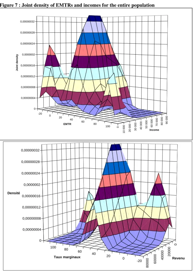
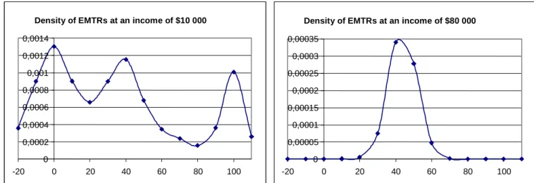
In order to extend our analysis and elaborate on the results mentioned above, a second graph allows us to study the distribution of the population as a function of two variables, the EMTR and family income. This graph is yielded by the estimation of a bivariate density. Observe Figure 7, in which we again find the three peaks that characterize the distribution of the population as a function of the tax rate. This new figure adds some information to our analysis. We see that households confronting rates that are either nil or 100 per cent are clearly concentrated in the lowest income brackets (i.e. between $0 and $20 000). In addition, rotating the graph (see the lower pane in Figure 7) reveals the presence of a single peak for medium- and high-income households. To verify this, we estimated the density of the EMTR conditional on income. This measure can be seen as a cross-section of the graph of the bivariate density at a given level of income. These results are presented in Figure 8. In the case of households whose family income is $10 000, we identify three zones of concentration at 0, 40, and 100 per cent, while those whose family income is $80 000 are all clustered around a single peak.
19 At the provincial level, the marginal rate of taxation on incomes between $26 701 and $53 405 is 20 per cent,
rising to then 24 per cent above $53 405. Federally, it is 22 per cent between $31 678 and $63 345, and then 26 per cent above $63 345. For the sum of the rates of the two levels of government to be 39 and 45 per cent, it is necessary to account for the Quebec tax abatement that reduces federal taxation.
Figure 7 : Joint density of EMTRs and incomes for the entire population -20 0 20 40 60 80 100 0 1 0 000 20 000 3 0 000 40 000 5 0 000 60 000 70 000 80 000 90 000 0 0,00000004 0,00000008 0,00000012 0,00000016 0,0000002 0,00000024 0,00000028 0,00000032 J oi nt de ns it y EMTR Income -20 0 20 40 60 80 100 0 20 000 40 000 6000 0 80 000 0 0,00000004 0,00000008 0,00000012 0,00000016 0,0000002 0,00000024 0,00000028 0,00000032 Densité
Figure 8 : Density of EMTRs conditional on income being $10 000 and $80 000
Density of EMTRs at an income of $10 000
0 0,0002 0,0004 0,0006 0,0008 0,001 0,0012 0,0014 -20 0 20 40 60 80 100
Density of EMTRs at an income of $80 000
0 0,00005 0,0001 0,00015 0,0002 0,00025 0,0003 0,00035 -20 0 20 40 60 80 100
4.2.1.2 Marginal rates by family status: the impact of the income distribution
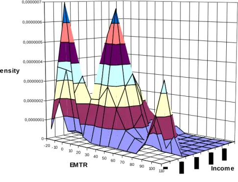
The four graphs presented in Figure 9 take our analysis yet further. They present the distribution of households as a function of EMTRs and income, by family status.
Although we do observe some occurrences amongst single-parent families, the majority of households facing a 100 per cent EMTR are those with no children (single individuals and childless couples). This is an interesting point, and merits that we pay some attention to the underlying explanations. At first blush, it appears plausible that the PWA program is a factor since, as we stated when presenting the representative agents, it contributes to lowering the marginal rate in the zone in which households are the beneficiaries of social assistance. After further investigation, however, it seems that the PWA program is not the reason for this result. In fact, we tested the sensitivity of our results for families by varying participation in the PWA program, from complete non-participation to full participation. Our results showed little sensitivity to these changes. While the PWA program has a significant impact on reducing the EMTR for some household types, as we saw before and as discussed in the literature by Bernier and Lévesque (1995), its impact remains minor in terms of the distribution of EMTRs amongst all families. Rather, the fact that households that are taxed at 100 per cent at the margin tend not to be families is explained as follows. Those for which we have a 100 per cent EMTR are largely those whose income is greater than $0 and less than $10 000 (households with one adult) or $15 000 (households with two adults). This applies to 26 per cent21 of single individuals, explaining
their prevalence in the 100 per cent EMTR group.
Figure 9 : Joint density of EMTRs and incomes, by status -20 -10 0 10 20 30 40 50 60 70 80 90 100 110 0 0,0000001 0,0000002 0,0000003 0,0000004 0,0000005 0,0000006 0,0000007 Density Incom e EMTR Single - 20 -10 0 10 20 30 40 50 60 70 80 90 100 110 0 0,00000005 0,0000001 0,00000015 0,0000002 0,00000025 0,0000003 0,00000035 0,0000004 0,00000045 0,0000005 Density Incom e EMTR Childless couple
-20 -10 0 10 20 30 40 50 60 70 80 90 100 110 0 0,00000005 0,0000001 0,00000015 0,0000002 0,00000025 0,0000003 D e ns i t y I nc ome E M T R Single parent 0 0,00000005 0,0000001 0,00000015 0,0000002 0,00000025 0,0000003 Density Incom e EMTR Single parent
Amongst single-parent families, 15 per cent are in this situation, while 24 per cent have a family income that is nil. For these latter, the maximum income allowed by social assistance is not reached when a $1000 rise in income is simulated. Consequently, their marginal rate is nil, or even negative, when the family qualifies for the PWA program but does not surpass a threshold beyond which it is penalized. Also, for single-parent families that are penalized (by the loss of some of the social assistance benefit), the PWA program effectively lowers the marginal rate to approximately 80 per cent.22 As to two-income
households, fewer of them have an income below $20 000 (9 per cent), which explains the low percentage among them with a marginal rate of 100 per cent. In summary, it is primarily the distribution of incomes unique to each group that explains why households with children are not typically taxed at a marginal rate of 100 per cent. Moreover, we should not forget that a hike in income of $5000 would leave over 80 per cent of families in a situation in which their effective tax rate, for a $1000 raise, would be nil.
We have mentioned that a significant proportion of single-parent families benefit from an EMTR equal to zero. We also find a significant concentration amongst single individuals. Once again, these households are generally those with zero family income. The greatest proportion is in households with a family income equal to zero among singles (10 per cent) and single-parent families (24 per cent). We also note that low income taxes are levied on youths aged 18 and plus who are not enrolled in post-secondary studies and live with their parents. With a mean EMTR of 25 per cent, these youths contribute to raising the proportion of single individuals faced with low EMTRs.
For the four household types, we observe significant clustering in the central zone of the graphs. However, close examination reveals that this clustering occurs around a different rate for each of the four groups. For single individuals and childless couples, the centre is at an EMTR of 40 per cent. For families, the greatest concentrations are at higher rates, 50 per cent for two-parent families and nearly 60 per cent for single-parent families. This result reflects the presence of many transfer programs that directly affect the family. We will discuss this in greater detail when we analyse the different components of the EMTR. When we examine the graph of the density of the marginal rates for the entire population, the zones of highest concentration are located around 39 and 45 per cent, i.e., below the levels that characterize families. This is because single individuals and childless couples represent 75 per cent of the weighted sample.
In conclusion, we point out that the distribution of rates is particularly smooth in the case of two-parent families. Since 73 per cent of them have a family income that exceeds $40 000, they are, for the most part, taxed at a rate of approximately 50 per cent at the margin. This rate is broken down into two components: income taxes levied by the two levels of government (45 per cent) and the CCTB (5 per cent). This reveals that, at the margin, the burden on two-parent families is already quite high. For the most part, their situation is such that only one half of income earned at the margin is available to them. Consequently, a reform of the tax and transfer systems that would increase the effective tax burden on medium- and high-income households would raise the EMTR, which is already high, on two-parent families.
4.2.2 The expected marginal rate as a function of income: an overview for each group
At this point, we are principally interested in the expected marginal rate as a function of family income. This allows a more targeted assessment of the impact a wage raise may have given a specific financial starting position. While the density measures we have already Thus, some families receiving social assistance may be taxed at a 100 per cent rate.
looked at shed light on the distribution of rates, estimating expected marginal rates reveals the expected level that the EMTR can attain for a given income level.
The first conclusion that arises when we observe the expected marginal rate for each of the four household groups is that, for some income brackets, families (whether headed by one or two parents) may be confronted with a marginal rate that exceeds the 50 per cent bar. This is not the case for singles and childless couples, as we see in Table 2.
Table 2: Expected marginal rate as a function of income, by family status
0 $ -10 000 $ 10 000 $ -20 000 $ 20 000 $ -30 000 $ 30 000 $ -40 000 $ 40 000 $ -50 000 $ 50 000 $ -60 000 $ 60 000 $ -70 000 $ 70 000 $ -100 000 $ Single 27.3 34.8 41.0 46.0 40.3 40.5 43.1 45.3 Single parent 14.9 49.7 57.3 59.6 53.4 49.1 49.4 48.9 Childless couples 41.8 36.0 36.6 42.1 40.0 39.3 40.2 41.3 Two-parent family 17.0 36.7 51.4 53.4 47.6 46.4 47.7 45.4 Total population 28.6 35.9 41.5 46.6 42.5 42.1 43.9 43.5
Overall, families face the highest average tax rates. Conversely, when household income is below $10 000, the expected rate on families is lower than that on childless households. It is within the group of single-parent families that the highest expected EMTR is observed. Between $15 000 and $45 000, the expected rate for this group remains above the 50 per cent threshold, reaching 62 per cent at $35 000 (cf. Figure 10).
As a rule of thumb, the expected rate varies significantly with the family status when income is below $50 000, while it converges to 45 per cent for all higher-income households.
Figure 10 : Expected marginal rate as a function of income, by family status
-5 0 5 10 15 20 25 30 35 40 45 50 55 60 65 0 10000 20000 30000 40000 50000 60000 70000 80000 90000 100000 Income E xp ect ed mar g in al r at e
4.2.3 The decomposition of the marginal rates and the impact of governmental assistance programs
In this section we present the decomposition of the expected EMTR for each of the four household types that we are interested in. This new phase of our analysis will yield the weight of each program and tax measure in the composition of the total rate.
The same EMTR for two different households does not necessarily imply an identical fiscal situation. For example, in Table 3 we see a single individual and a single-parent family both facing the same expected EMTR, 35 per cent. For the single individual, income taxation represents nearly 60 per cent of the mean marginal rate, while this share is 50 per cent for the single-parent family. Though the share of the marginal dollar earned that must be remitted in taxes is smaller than for the single person, the single-parent family loses out on transfer payments it had been receiving. In fact, on an additional $1 in labour income, it will pay $0.17 in income taxes on average ($0.21 for a single individual), $0.03 in various premiums ($0.04 for singles) and forfeit $0.13 in transfers ($0.11 for singles), yielding the same marginal rate for both groups.
Table 3: Decomposition of the mean effective rate, by family status
Two-parent family
Single Single parent Childless couple All households
Decompo-sition of the total rate Decompo-sition of the total rate Decompo-sition of the total rate Decompo-sition of the total rate Decompo-sition of the total rate Proportion of the total rate Proportion of the total rate Proportion of the total rate Proportion of the total rate Proportion of the total rate
Compared to the household consisting of a single adult, the mean marginal rate on a childless couple and a two-parent family is higher by 5 and 10 per cent, respectively. Also observe that marginal income tax rates are higher for households headed by two adults. Furthermore, marginal income taxation distinguishes the single-parent family from the two-parent family. The clawback rate on transfer programs is less for the latter. It is the greater wealth, on average, of families with two adults that explains the different composition of the mean marginal rate (recall from Figure 5 how the average income of the head of a single-parent family is lower than that of a two-single-parent family). With a mean income level near $25 000 (earned by the head of a single-parent family), the income tax rate for both levels of
Fédéral tax 10,6 30% 8,7 25% 14,2 36% 15,6 35% 12,5 33% Provincial tax 10,3 29% 8,6 25% 15,0 38% 16,1 36% 12,6 33% 3,9 Dues (1) 3,8 11% 3,4 10% 3,6 9% 9% 3,7 10% Income assistance programs (2) 10,5 30% 5,9 17% 6,1 15% 3,0 7% 7,7 20% Children related programs ( 3) 0,0 0% 7,4 21% 0,0 0% 5,1 11% 1,3 3%
Tax credits and
refunds (4) -0,3 -1% 0,8 2% 1,0 3% 1,4 3% 0,5 1%
TOTAL 35,0 100% 34,7 100% 39,9 100% 45,0 100% 38,2 100%
(1) Employment-insurance, QPP and drugs insurance
(2) Social assistance, PWA, PWA supplement and housing allowance
(3) CCTB, supplement for young child, family allowances, daycare and credit for childcare expenses (4) GST credit, QTS credit and property tax refund
government is relatively low (amounting to 50 per cent of the global rate for a single-parent family), but the implicit rate on several income and family support programs starts to make itself felt (accounting for 41 per cent of the total rate on the single-parent family). At the other extreme, when income is approximately $50 000 (earned by the head of a two-parent family), income tax rates are higher (accounting for 70 per cent of the global rate confronting the two-parent family), while the clawback rate on government programs is nearly nil (accounting for 21 per cent of the overall rate for the two-parent family).
As to the 5 per cent difference between the marginal rate on childless couples and two-parent couples, it is primarily explained by the presence of children. These make it possible for parents to access assistance programs whose payoffs decrease with rising family income, resulting in an implicit tax rate of 5 per cent. Aside from this difference, which explains the gap between the total rate, we also note that the composition of the mean rates is not exactly the same. Since the income of both members of childless couples is below that of the parents of two-parent families (cf. Figure 5), the implicit rate on income assistance programs is greater for the former, while the rates associated with income taxation are greater for the latter.
4.2.4 The variability of EMTRs
The variability of EMTRs can be analysed from several perspectives. First, we observe this variability of rates within our household groupings (by family status). Is there uniformity in marginal taxation, or do we find some types of inequality between households in the same group? Subsequently, we also analyse the degree of variability of EMTRs across the four groups. With all income categories considered, is there a form of inequality between these groups? Finally, we address the disparity of implicit rates within various groupings of programs and fiscal measures (for example: all income support measures, all programs targeted at children, etc.), as well as the interactions between these groupings.
To analyse the variability of the EMTRs we use a generalized entropy index (cf., Fournier [2005] for more information on the indices used). An entropy index is a measure of dispersion or distance with respect to a centre (or mean). It captures the degree of disorder or inequality that reigns in a system. Thus, the entropy index will be zero if the EMTR is the same for everyone and high if differences between the rates and their means are large. Furthermore, a decomposition of the generalized entropy index allows inter-group inequality to be distinguished from intra-group inequality.23
Table 4 presents the principal entropy measures we estimated. The first column shows the entropy estimate for each household type. The second column provides the normalized mean, which is the ratio of the mean of the marginal rate within the group to the mean rate for the entire population. The third column is the share of each group in the total population. The fourth and fifth columns summarize the decomposition of total inequality by indicating, in absolute and relative terms, the contribution of each group (as well as between-group
23 Estimates of the entropy measures and other computations were generated with the software DAD (for
Distributive analysis/Analyse distributive). DAD was designed to facilitate the analysis and comparisons of social welfare, inequality, poverty, and equity across various population distributions. For more information regarding DAD, as well as equity and poverty measures, consult Duclos and Araar (2006).
inequality) to total inequality. We first observe the value assumed by the entropy index for each of the four groups. This index is highest for the group of single-parent families (0.805). Thus, it is within this group that the greatest variation in EMTRs is found. Recall that single-parent families are distributed between two main peaks. Many of them are in a situation of zero marginal taxation, while we also find a significant concentration around 60 per cent. The considerable distance between these two points of concentration explains the high entropy index. Single individuals occupy second place (0.578) in terms of an unequal distribution of rates. We can also explain this result by their distribution between effective marginal tax rates of zero and of 40 and 100 per cent. Finally, childless couples (0.195) and two-parent children (0.157) are in third and fourth place, respectively, in terms of the dispersion of tax rates. Density graphs for these two groups support this result (cf. Figure 9).
Table 4: Entropy measures and decomposition of the inequality of the EMTRs
Groups Estimate of entropy Normalised mean Proportion Absolute contribution Relative contribution Single 0,578 0,954 0,488 0,269 68,0% Single parent 0,805 1,021 0,040 0,033 8,2% Childless couple 0,195 1,007 0,285 0,056 14,1% Two-parent 0,157 1,097 0,188 0,032 8,2% Between-group inequality - - - 0,006 1,4% Total inequality 0,395 100,0%
The wide variability of the rates and the distribution of the households between very distant peaks of taxation for single individuals and single-parent families can be explained by the high proportion of low-income households we find in these two groups, compared to households with two adults. For each of those two groups we also computed the entropy index for family income. We observe that the groups with the greatest income disparity are also those in which we find the greatest disparities in the EMTRs.
The inequality index for the whole population is 0.395. This index is the sum of two components: within-group and across-group inequality. Beginning with the first component, we first determine the relative contribution of each group in the population to the total inequality index. Single individuals have an index rate dispersal that is relatively high compared to the others. Since they also include 49 per cent of households, they contribute most to the variation in the rates. Single-parent families—the group within which disparities are greatest—contribute very little to the total inequality index owing to the small percentage of the population they represent (4 per cent). The second component is the share of the inequality attributable to the variation in the rates between groups. We observe that this component only contributes 1.4 per cent of total inequality. The fact that the normalized means are very near to one (1) also attests to the absence of inter-group inequality. In comparison, income disparity across groups contributes 26.2 per cent to the total income inequality within the population. Thus, while the distribution of mean incomes between groups presents a certain degree of inequality, it appears that, on average, the EMTRs vary very little across groups.
Finally, we note that, while two-parent families face expected marginal rates that are relatively high compared to the other groups, it appears that there is little variation in the marginal rates confronting these families. Conversely, it is within this group that the variance in the marginal rate is greatest in the case of low incomes. This is what we see in Figure 11, which illustrates the standard deviation of the conditional marginal rates for a given income and family status.
Figure 11 : Standard deviation of the marginal rates, conditional on a given income, by family status
Figure 11 also shows the variability of EMTRs for low-income single-parent families. Compared to childless households, the fiscal situation of families is more variable in the lower income brackets in terms of marginal taxation for a given income. Overall, the reduced disparity amongst two-parent families is primarily attributable to the fact that they are richer than single-parent families. Finally, Figure 11 presents the relative invariability of EMTRs for medium- and high-income households.
0 20 40 60 80 100 120 140 0 10000 20000 30000 40000 50000 60000 70000 80000 90000 10 S ta nda rd d e v ia ti on of E M TR s
Two-parent Childless couples Single-parent Singles
It is instructive to analyse the variance of rates within various groupings of programs and fiscal measures. We created six groups:
1) programs pertaining to children (including the CCTB, the federal government’s young child supplement, as well as family allowances from the provincial government); 2) income support programs (including social assistance, the PWA24 program, and
housing allowance, all of which are administered by the provincial government);