HAL Id: hal-00693154
https://hal.archives-ouvertes.fr/hal-00693154
Submitted on 2 May 2012
HAL is a multi-disciplinary open access
archive for the deposit and dissemination of
sci-entific research documents, whether they are
pub-lished or not. The documents may come from
teaching and research institutions in France or
abroad, or from public or private research centers.
L’archive ouverte pluridisciplinaire HAL, est
destinée au dépôt et à la diffusion de documents
scientifiques de niveau recherche, publiés ou non,
émanant des établissements d’enseignement et de
recherche français ou étrangers, des laboratoires
publics ou privés.
Stiffness Modeling of Robotic-Manipulators Under
Auxiliary Loadings
Alexandr Klimchik, Anatol Pashkevich, Stéphane Caro, Damien Chablat
To cite this version:
Alexandr Klimchik, Anatol Pashkevich, Stéphane Caro, Damien Chablat.
Stiffness Modeling of
Robotic-Manipulators Under Auxiliary Loadings. The ASME 2012 International Design Engineering
Technical Conferences (IDETC) and Computers and Information in Engineering Conference (CIE),
Aug 2012, Chicago, United States. �hal-00693154�
STIFFNESS MODELING OF ROBOTIC-MANIPULATORS
UNDER AUXILIARY LOADINGS
Alexandr Klimchika,b, Anatol Pashkevicha,b, Stéphane Carob, Damien Chablatb a
Ecole des Mines de Nantes, 4 rue Alfred-Kastler, 44307 Nantes, France b
Institut de Recherches en Communications et Cybernétique de Nantes, UMR CNRS 6597, France
KEYWORDS
Stiffness analysis, passive joints, auxiliary loading, static equilibrium, non-linear stiffness model.
ABSTRACT
The paper focuses on the extension of the virtual-joint-based stiffness modeling technique for the case of different types of loadings applied both to the robot end-effector and to manipulator intermediate points (auxiliary loading). It is assumed that the manipulator can be presented as a set of compliant links separated by passive or active joints. It proposes a computationally efficient procedure that is able to obtain a non-linear force-deflection relation taking into account the internal and external loadings. It also produces the Cartesian stiffness matrix. This allows to extend the classical stiffness mapping equation for the case of manipulators with auxiliary loading. The results are illustrated by numerical examples.
1. INTRODUCTION
Manipulator stiffness modeling under internal and external loading is a relatively new research area that is important both for serial and parallel robots. In general case, these loadings may be of different nature and applied to different points/surfaces. For the stiffness modeling of robotic manipulator, it is reasonable to distinguish three main types of loading such as external loading applied to end-point, preloading in the joints and auxiliary loading applied to the intermediate points.
The external loading is caused mainly by an interaction between the robot end-effector and the workpiece, which is
processed or transported in the considered technological process [1]. In most of robotic research works this loading is considered as a unique one [2] [3], however existence and effect of other types have not been discussed yet.
The internal loading in some joints may be introduced by the designer. For instance, to eliminate backlash, the joints may include preloaded springs, which generate the force or torque even in standard "mechanical zero" configuration [4]. Though the internal forces/torques do not influence on the global equilibrium equations, they may change the equilibrium configuration and also influence on the manipulator stiffness properties. For this reason, internal preloading is used sometimes for the purpose of improving the manipulator elasto-static properties, especially in the vicinity of kinematic singularities. Another case where the internal loading exists by default, is related over-constrained manipulators that are subject of the so-called antagonistic actuating [5]. Here, redundant actuators generate internal forces and torques that are equilibrated in the frame of closed loops.
The term auxiliary loading, in this paper, is used to denote external loading applied to any intermediate point (surface, etc.) of the manipulator different from the end-effector. Typical example of such type of loading is the gravity that is non-negligible for heavy manipulators employed in machining applications [6]. Besides, to compensate in certain degree the gravity influence, some manipulators include special mechanisms generating external forces/torques in the opposite direction (gravity compensators). In addition, some additional forces/torques may be generated by other sources (geometrical constrains, for instance). It should be noted that the external loading caused by gravity has obvious distributed nature, but usually it can be approximated by lumped forces that applied to one or several intermediate points.
From point of view of stiffness analysis, the external and internal forces/torques directly influence on the manipulator equilibrium configuration and, accordingly, may modify the stiffness properties. So, they must be undoubtedly be taken into account while developing the stiffness model. However, in most of the related works the Cartesian stiffness matrix has been computed for the nominal configuration, which does not take into account influence of external/internal loading. Such approach is suitable for the case of small deflections only. For the opposite case, the most important results have been obtained in [7-10], which deal with the stiffness analysis of serial and parallel manipulators under the end-point loading. Besides, some types of the internal preloading have been in the focus of [11], [12]. However, influence of the auxiliary loading has not been studied in details yet.
To our knowledge, the most advanced stiffness model for robotic manipulator has been proposed in [6], where numerous factors have been taken into account (conventional external loading, gravity forces, antagonistic redundant actuation, etc.). However, proposed approach is hard from computational point of view. Besides, in this work the Jacobians and all their derivatives were computed not in a "true" equilibrium configuration. For this reason, since the equilibrium obviously depends on the loading magnitude, some essential issues have been omitted.
The goal of this work is to generalize the non-linear stiffness modeling technique for the case of three types of loadings: (i) the external loading applied to the end-effector, (ii) preloading in the joints and (iii) auxiliary loading applied to the intermediate node-points. The developed model is based on the VJM-technique proposed in [13], which is able to obtain the force-deflection relation and the manipulator Cartesian stiffness matrix assuming that the external loading is applied to the end-effector only.
2 PROBLEM STATEMENT
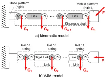
For stiffness modeling of serial kinematic chain with the loading applied to end-point, preloading in the joints and auxiliary loading applied to intermediate points let us use the VJM model that is presented in Fig.1. The serial chain under study consists of flexible links separated by passive and/or actuated joints. Its geometry (end-point location) is described by the vector function
( , )
t g q θ (1) where the vector t defines the end-point location (position and orientation (Euler angles)); the vectors
q T 1 2 n (q, q , ..., q ) q and θ T 1 2 n ( , , ..., )
θ collect all passive and virtual joints coordinates respectively; nq, nθ are the sizes of q and θ,
respectively.
Figure 1 General structure of kinematic chain with auxiliary loading and its VJM model
Stiffness modeling for the manipulators with end-point loading and preloading in the joints have been already published in [13], However other types of loadings (here they are aggregated in the auxiliary loading) applied to intermediate points did not receive adequate attention in robotics. In practice, these loadings can be caused by gravity forces (generally they are distributed, but in practice they can be approximated by localized ones) and/or gravity compensators. These forces will be denoted as Gj, where j1, ...,n is the
node number in the serial chain starting from the fix base (here, j n corresponds to the end-point). It should be noted that for computational convenience, it is assumed that the end point loading consists of two components Gn and F of different
nature.
It is evident that in general the auxiliary forces Gi depend
on the manipulator configuration. So, let us assume that they are described by the functions
( , ) j j
G G q θ , (2) In contrast, for the external force F, it is assumed that there is no direct relation with manipulator configuration.
For the serial chains with auxiliary loadings it is also required to extend the geometrical model. In particular, in addition to equation (1) defining the end-point location, it is necessary to introduce additional functions
( , ), 1, ..., j j j n
t g q θ (3)
defining locations of the nodes. It worth mentioning that for the serial chain, the position tj depends on a sub-set of the joint
coordinates (corresponding to the passive and virtual joints located between the base and the j-th node), but for the purpose of analytical simplicity let us use the whole set of the joint coordinates ( ,q θ) as the arguments of the functions gi(...).
Using these assumptions and using results from our previous works [13][14], the problem of the manipulator stiffness modeling with auxiliary loadings can be split into several steps that are sequentially considered in the following sections.
3 STATIC EQUILIBRIUM EQUATIONS
To obtain a desired stiffness model, it is required to derive the static equilibrium equations that differ from the one used for the end-point loaded manipulator only due to influence of auxiliary loadings Gj. Let us apply the principle of the virtual
work and assume that the kinematic chain under external loadings F and G
G1...Gn
has the configuration
q θ,
and the locations of the end-point and the nodes are t g q θ( , )
and tj gj( , ),q θ j1,n respectively.
Following the principle of virtual work, the work of external forces G F, is equal to the work of internal forces τ caused by displacement of the virtual springs δθ
T
T T θ 1 δ δ δ n j j j
G t F t τ θ (4)where the virtual displacements δtj can be computed from the
linearized geometrical model derived from (3)
( ) ( )
θ q
δ j δ j δ , 1.. j j n
t J θ J q , (5) which includes the Jacobian matrices
( ) ( ) θ , ; q , j j j j J g q θ J g q θ θ q (6)with respect to the virtual and passive joint coordinates respectively.
Substituting (5) to (4) we can get the equation
T ( ) T ( ) θ q 1 T ( ) T ( ) T θ q θ δ δ δ δ δ n j j j j j n n
G J θ G J q F J θ F J q τ θ (7)which has to be satisfied for any variation of δ , δθ q. It means that the terms regrouping the variables δ , δθ q have the coefficients equal to zero, hence the force-balance equations can be written as ( ) T ( ) T ( ) T ( ) T θ θ θ q q 1 1 ; n n j n j n j j j j
τ J G J F 0 J G J F (8)These equations can be re-written in block-matrix form as
(G ) T (F) T (G ) T (F) T θ θ θ ; q q τ J G J F 0 J G J F (9) where (F) ( ) ( ) ( ) (G ) (1) ( ) θ θ q q θ θ θ (G ) (1) T T T T T T ( )T T T q q q 1 ; ; ... ; ... ; ... n F n n n n J J J J J J J J J J G G G (10)
Finally, taking into account the virtual spring reaction
0
θ θ τ K θ θ , where
1 n θ diag θ , ..., θ K K K , the desired static equilibrium equations can be presented as
(G ) T (F ) T 0 θ θ θ (G ) T (F ) T q q J G J F K θ θ J G J F 0 (11)Further, these equations will be used for computing the static equilibrium configuration and corresponding Cartesian stiffness matrix.
4 STATIC EQUILIBRIUM CONFIGURATION
To obtain a relation between the external loading F and internal coordinates of the kinematic chain ( , )q θ
corresponding to the static equilibrium, equations (11) should be solved either for different given values of F or for different given values of t. In [13] these problems were referred to as the original and the dual ones respectively, but the dual problem was discovered to be the most convenient from computational point of view. Hence, let us solve static equilibrium equations with respect to manipulator configuration
q θ,
and external loading F for given end-effector position tg q θ
,
and function of auxiliary-loadings G q θ
,
0 (G ) T (F ) T θ θ θ (G ) T (F ) T q q ; , ; , K θ θ J G J F J G J F 0 t g q θ G G q θ (12)where the unknown variables are
q θ F, ,
.Since usually this system has no analytical solution, iterative numerical technique can be applied. So, the kinematic equations may be linearized in the neighborhood of the current configuration (qi,θi)
(F) θ (F 1 q 1 1 ) , , , ; i i i i i i i i i i i t g q θ J q θ θ θ J q θ q q (13)where the subscript 'i' indicates the iteration number and the changes in Jacobians (G ) (F) (G ) (F)
θ , θ , q , q
loadings G q θ
,
are assumed to be negligible from one iteration to another. Correspondingly, the static equilibrium equations in the neighborhood of (qi,θi) may be rewritten as
(G ) T (F ) T 0 θ θ θ (G ) T (F ) T q 1 q 1 1 i i i J G J F K θ θ J G J F 0 . (14)Thus, combining (13) and (14), the iterative algorithm for computing of static equilibrium configuration for given end-effector location can be presented as
1 (F ) (F ) q θ (F ) T (G ) T q q (F ) T (G ) T 0 θ θ θ θ (F ) (F 1 1 1 ) q 1 , θ · i i i i i i i i i i 0 J J ε F q J 0 0 J G θ J 0 K J G K θ ε t g q θ J θ J q (15) where Gi1G q( i1,θi1).To reduce the size of a matrix to be inverted, the above system can be slightly simplified. In particular, based on analytical expression for 1 (G ) T (F) T 0
θ ( θ θ )
θ K J G J F θ , the unknown variables can be separated in two groups ( ,F q) and
θ . This yields the iterative scheme
1 (F ) 1 (F ) T (F ) θ θ q (G ) T (F ) T q q 1 (G ) T (F ) T 0 θ θ θ (F ) (F ) (F ) 1 (G ) T θ q θ θ 1 1 1 1 1 , · i i i i i i i i i i i i J K J J ε F J G q J 0 θ K J G J F θ ε t g q θ J θ J q J K J G (16)that requires matrix inversion of essentially lower order (for example, for 3-link manipulator with two passive joints and two actuated joints, the size of matrix inversion reduces from 34 to 14). It should be mentioned that 1
θ
K is computed only once, outside of the iterative loop. The proposed algorithm allows us to compute static equilibrium configuration for the serial chains with passive joints and all types of loadings (internal preloading, external loadings applied to any point of the manipulator and loading from the technological process).
5 STIFFNESS MATRIX
Previous Section allows us to obtain the non-linear relation between elastic deflections Δ t and external loading F . In order to obtain the Cartesian stiffness matrix, let us linearize the force-deflection relation in the neighborhood of the equilibrium. Following this approach, two equilibriums that correspond to the manipulator state variables ( ,F q θ t, , ) and
(Fδ ,F qδ ,q θδ ,θ tδ )t should be considered simultaneously. Here δF, δt define small increments in the external loading and relevant displacement of the-end-point.
Using this notation, the static equilibrium equations may be written as
0
(G ) T (F ) T θ θ θ (G ) T (F ) T q q , t g q θ K θ θ J G J F J G J F 0 (17) and
T 0 (G ) (G ) θ θ θ T (F ) (F ) θ θ T T (G ) (G ) (F ) (F ) q q q q δ δ , δ δ δ δ δ δ δ δ δ δ t t g q q θ θ K θ θ θ J J G G J J F F J J G G J J F F 0 (18) where 0 θ , , , , , ,t F G K q θ θ are assumed to be known.
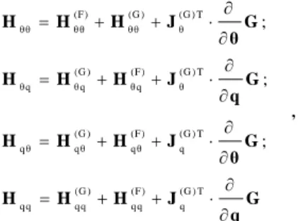
After linearization of the function g q θ( , ) in the neighborhood of loaded equilibrium, the system (17), (18) is reduced to three equations
(F) (F) θ q (G ) (G ) (F) (F) θ θ θ θ θ (G ) (G ) (F) (F) q q q q δ δ δ δ δ δ δ δ δ δ δ δ t J θ J q K θ J G J G J F J F J G J G J F J F 0 (19)
which define the desired linear relations between δt and δF,
δ q, δθ that are expressed via the stiffness matrices KC, KC q, C θ
K . In this system, small variations of Jacobians may be expressed via the second order derivatives
(F ) (F ) (F ) (F ) (F ) (F ) q q θ qq θ θθ θq (G ) (G ) (G ) (G ) (G ) (G ) q q θ qq θ θθ θq δ δ δ ; δ δ δ ; δ δ δ ; δ δ δ ; J H θ H q J H θ H q J H θ H q J H θ H q (20) where
2 2 (G ) (F ) θθ θθ 1 2 2 (G ) (F ) q q q q 1 2 2 (G ) (F ) θq θq 1 2 2 (G ) (F ) q 2 2 2 θ qθ 1 2 ( , ) ; ( , ) ( , ) ; ( , ) ( , ) ; ( , ) ( , ) ; ( , ) n j j n j j n j j n j T T j T T j T T j T T j j
H g q G H g q F θ θ H g q G H g q F q q H g q G H g q F θ q θ q H g q G H g q F q θ q θ θ θ θ θ θ θ θ θ (21)Also, the auxiliary loading G may be computed via the first order derivatives as
Further, let us introduce additional notations (F ) (G ) (G ) T θθ θθ θθ θ (G ) (F ) (G ) T θq θq θq θ (G ) (F ) (G ) T q θ qθ qθ q (G ) (F ) (G ) T q q q q q q q ; ; ; H H H J G θ H H H J G q H H H J G θ H H H J G q , (23)
which allows us to present system (19) in the form
(F ) (F ) q θ (F ) T q q q q θ (F ) T θ θq θ θθ δ δ δ δ 0 J J t F 0 J H H q 0 J H K H θ (24)
that has the same structure as for end-point loaded manipulator [13]. Hence, similarly the desired Cartesian stiffness matrices
C
K and stiffness matrices KC θ and KC q defining linear
mappings of end-point displacement δ t to internal coordinates deflections δθ and δ q:
C θ ; C q
δθK δt δqK δt (25) can be computed via either high order matrix inversion
1 (F ) (F ) q θ C (F ) T C q q q q q θ (F ) T C θ θ θq θ θθ * * 0 J J K K J H H K J H K H (26)
or lower order inversion
1 (F) F (F) T (F) (F) F C θ θ θ q θ θ θq (F) T F (F) T F C q q qθ θ θ qq qθ θ θq K J k J J J k H K J H k J H H k H (27) where F 1 θ ( θ θθ)
k K H denotes the modified joint compliance matrix. It is obvious that, using these notations, the matrices
C
K , KC q, KC θ can be also computed analytically using the
block matrix inversion [15]
0 ( ) 0 ( ) F F C q θ θ θq · C q F F C C K K K J J k H K (28) where 0(F ) F T 1 C ( θ θ θ) K J k J defines stiffness of the kinematic chain without passive joints [2], [3] and
F T F T C q qq q θ θ θq q qθ θ θ 0(F) F T F T 0(F) C q θ θ θq q qθ θ θ C 1 · K H H k H J H k J K J J k H J H k J K (29)Similarly, the matrix K can be expressed analytically as
F T F
C θ θ θ C θ θq C q
K k J K k H K (30)
Hence, the technique presented in this Section allows us to compute Cartesian stiffness matrix KC and stiffness matrices
C θ
K and KC q defining linear mappings of end-point
displacement δ t to internal coordinates deflections δθ and
δ q for manipulators with external and internal loading applied to the intermediate nod-points (auxiliary loading). Presented approach deals with serial chains, however obtained results can be easily transferred to a parallel manipulators using aggregation technique from [13].
6 ILLUSTRATIVE EXAMPLES
Let us now focus on the non-linear stiffness analysis of a serial chains under auxiliary loadings applied to an intermediate node. It is assumed that the considered chain consists of two links (either rigid or flexible) separated by a flexible joint. Relevant analysis includes evaluating stiffness variation due to the loading, detecting of buckling and computing corresponding critical forces, as well as analysis of the auxiliary spring influence on the chain stiffness.
6.1 Serial chain with torsional springs
Let us consider first a 2-link manipulator with a compliant actuator between the links and two passive joints at both ends. It is assumed that the left passive joint is fixed, while the right one can be moved along x direction (Fig.2a). Besides, here both rigid links have the same length L and the actuator stiffness is
θ
K .
Figure 2 Kinematic chains with compliant actuator between two rigid links (a) and compliant actuator between two
compliant links (b)
Let us assume that the initial configuration (i.e. for
0
M ) of the manipulator corresponds to 0 / 6 , where
2·
is the coordinate of the actuated joint. It is also assumed that the external loading G is applied to the intermediate node (Fig.2a) and it is required to apply the external loading (Fx,Fy) at the end-point to compensate the
auxiliary loading G. Since this example is quite simple, it is possible to obtain the force-deflection relation and the stiffness coefficient both analytically and numerically.
For this manipulator the force-displacement relation can be expressed in a parametric form as
θ 0 co s · 2· · ; ; 2 sin sin 2 x y K G G F F L (31)
and stiffness of the manipulator can be presented as
θ 3 3 0 2 ·co s sin 1 · · 4 sin sin x K G K L L (32)where ( / 2; / 2 ) is treated as a parameter and Ky 0.
As follows from expression (32), the stiffness coefficient
x
K essentially depends on the auxiliary loading G. In particular, for the initial configuration, the coefficient Kx can
be both positive and negative or even equal to zero when the auxiliary loading is equal to its critical value
θ *
0
4 / ·sin
G K L . It is evident that the case *
G G is very dangerous from practical point of view, since the chain configuration is unstable.
Figure 3 Force-deflections relations for different values of auxiliary loading G : chain with torsional spring
( *
θ 0
4 / ·sin
G K L , KxK K· θ/L2)
Summarized results for this case study are presented in Fig.3 that contain the force-deflection relations and values of translational stiffness Kx respectively. They show that the
auxiliary loading G significantly reduces the stiffness of the serial chain. For example, in initial configuration ( x 0), for
0 G the stiffness is 2 θ 1 4 .9 ·K /L , while for * 0.5· G G it reduces down to 2 θ
8 .6 7 ·K /L . Further increasing of the auxiliary loading up to *
1.5·
G G leads to the unstable configuration with negative stiffness 2
θ
7 .4 6 ·K /L
. Moreover, in the neighborhood of the critical value of *
G G , the force-deflection curves have extremum points which may provoke buckling.
For this case study, similar analysis has been also performed using the developed numerical technique presented in section IV and V. It worth mentioning that the numerical technique yielded the same results as the analytical one, which confirms validity of the developed approach. Some details concerning functions and matrices used in relevant expressions are presented in Table 1, whereL1 and L2 denote the
manipulator link lengths, q1 and q2 are the passive joint
coordinates, is the virtual spring coordinate and 0 is the
actuator coordinate. It is worth mentioning that the numerical
technique yielded the same results as the analytical one, which confirms validity of the developed approach.
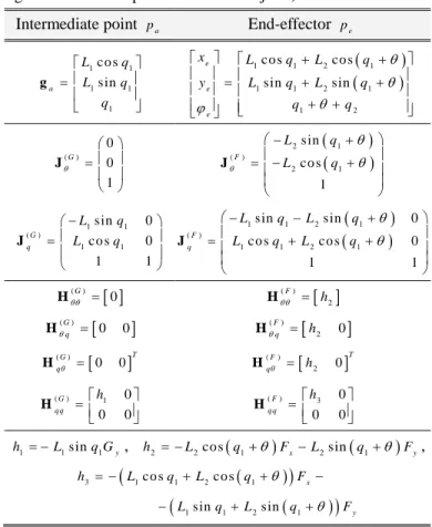
Table 1 Functions and matrices used in numerical stiffness analysis of two-link manipulator with auxiliary loading (case of rigid links and compliant intermediate joint)
Intermediate point pa End-effector pe
1 1 1 1 1 co s sin a L q L q q g
1 1 2 1 1 1 2 1 1 2 co s co s sin sin e e e L q L q y L q L q x q q ( ) 0 0 1 G J
2 1 ( ) 2 1 sin co s 1 F L q L q J 1 1 ( ) 1 1 sin 0 co s 0 1 1 G q L q L q J
1 1 2 1 ( ) 1 1 2 1 sin sin 0 co s co s 0 1 1 F q L q L q L q L q J
( ) 0 G H H(F)
h2
( ) 0 0 G q H H(Fq)
h2 0
( ) 0 0 G q T H ( )
2 0
F q T h H ( ) 1 0 0 0 G q q h H ( ) 3 0 0 0 F q q h H 1 1sin 1 y h L q G , h2 L2cos
q1
Fx L2sin
q1
Fy,
3 1 1 2 1 1 1 2 1 co s co s sin sin x y L q L q L q L q h F F Hence, the presented case study demonstrates rather interesting features of stiffness behavior for kinematic chains under auxiliary loading that where not studied before (negative stiffness, non-monotonic force-deflection curves, etc.). This motivates considering more sophisticated examples, with more complicated compliant elements.
6.2 Serial chains with torsional and translational springs
In the second example, it is assumed that there are three compliant elements: an actuated joint with torsional stiffness parameter Kθ and two non-rigid links with translational
stiffness KL (Fig.2b). Intuitively, it is expected that such system
should demonstrate more complicated stiffness behavior under the loadings compared to the previous one.
The force-deflection relations corresponding to serial chain with compliant links are presented in Fig.4. These curves have been obtained using functions and matrices presented in Table 2. Compared to the previous case, here for *
0...
only quantitative difference (i.e. the shape of the examined curves remains almost the same). However, for *
G G the chain may be not only unstable with respect to end-effector loading Fx, but also the chain configuration may become
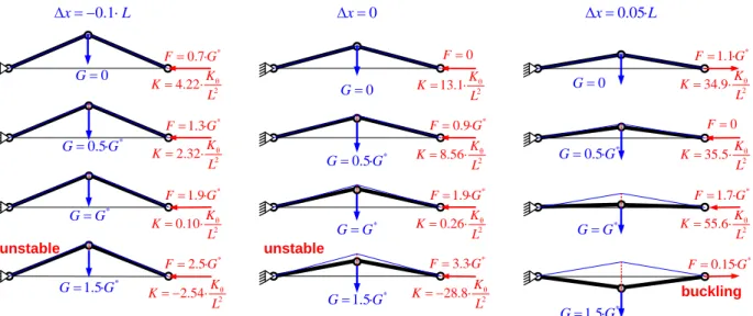
unstable. Geometrically, the latter qualitative difference is observed similar to buckling in vertically loaded arch. Summary of different chain configurations and their stiffness behavior is presented in Figure 5.
Figure 4 Force-deflections relations for different values of auxiliary loading G : chain with torsional and translational
springs ( * θ 0 4 / ·sin G K L , 2 θ · / L K K K L )
Summarizing Section 6, it should be concluded that auxiliary loading essentially influences on the stiffness behavior of robotic manipulators, may reduce the stiffness coefficient and also provoke undesirable phenomena (such as buckling) that must be taken into account by designers. This justifies results of this paper and gives perspectives for practical applications.
7 CONCLUSION
The paper presents generalization of the non-linear stiffness modeling technique for manipulators under internal and external loadings. The developed technique includes computing of the static equilibrium configuration corresponding to the loadings. It is able to obtain the non-linear force-deflection relation, the Cartesian stiffness matrix for the loaded mode as well as the matrices defining linear mappings from the end-point displacement into the deflections in passive and virtual joints. The obtained results allow us to extend the classical notion of "conservative congruence transformation" for the case of manipulators with auxiliary loading.
The advantages and use of the developed technique are illustrated by numerical examples that deal with a stiffness analysis of serial chains with different assumptions on the link flexibility. For the considered cases, functions and matrices that are used in numerical stiffness analyses are given. The presented results also illustrate the ability of this technique to detect some nonlinear effects in the manipulator stiffness behavior (such as buckling).
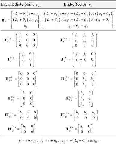
Table 2 Functions and matrices used in numerical stiffness analysis of two-link manipulator with auxiliary loading (case of rigid links and compliant intermediate joint)
Intermediate point pa End-effector pe
11 11
1 1 co s sin a L q L q q g
11 11
11
22 33
11 22
1 2 2 co s co s sin sin L q L q L q L q q q 1 ( ) 2 0 0 0 0 0 0 0 G j j J 1 5 7 ( ) 2 6 8 0 1 0 F j j j j j j J 3 ( ) 4 0 0 1 1 G q j j J 3 5 ( ) 4 6 0 0 1 1 F q j j j j J ( ) 0 0 0 0 0 0 0 0 0 G H ( ) 3 4 4 0 0 0 0 0 0 F h h h H 1 ( ) 0 0 0 0 0 G q h H 5 ( ) 3 4 0 0 0 F q h h h H ( ) 1 0 0 0 0 0 G q h H ( ) 5 3 4 0 0 0 F q h h h H ( ) 2 0 0 0 G q q h H ( ) 6 0 0 0 F q q h H 1 co s 1 j q , j2sinq1, j3
L11
sinq1,
4 1 1 cos 1 j L q , j5
L23
sin
q12
,
6 2 3 cos 1 2 j L q , j7 cos
q12
,
8 sin 1 2 j q h1 Gxsinq1Gyco sq1,
2 x 1 1 cos 1 y 1 1 sin 1 h G L q G L q ,
3 x 2 3 cos 1 2 y 2 3 sin 1 h F L q F L q ,
4 xsin 1 2 ycos 1 h F q F q , 5 Fxsinq1 Fyco sq1 h ,
6 3 x 1 1 cos 1 y 1 1 sin 1 h h F L q F L qIn future, it is reasonable to develop an extension of the proposed technique that can be applied to the parallel manipulators with internal loops. Besides, it is useful to consider the manipulators with several points (or end-effectors). The main difficulty for both cases is related to the introducing of additional geometrical constraints that are defined by another compliant mechanism.
unstable buckling * 0.5· G G * GG * 1.5· G G 0 F * 1.7· F G * 0.15· F G * 0.9· F G * 1.9· F G * 3.3· F G * 1.3· F G * 1.9· F G * 2.5· F G * 0.5· G G * 0.5· G G * GG * GG * 1.5· G G * 1.5· G G θ 2 2.32·K K L θ 2 0.10·K K L θ 2 2.54·K K L θ 2 28.8·K K L θ 2 0.26·K K L θ 2 8.56·K K L θ 2 35.5·K K L θ 2 55.6·K K L unstable 0 G 0.1 x L * 0.7· F G θ 2 4.22·K K L 0 x 0 F 0 G 13.1· 2θ K K L 0.05· x L * 1.1· F G 0 G θ 2 34.9·K K L
Figure 1 Figure 5 Configuration of kinematic chain with auxiliary loading: case of torsional and translational springs ( * θ 0 4 / ·sin G K L , 2 2 θ 2·1 0 · / L K K L ) ACKNOWLEDGMENT
The work presented in this paper was partially funded by the Region “Pays de la Loire” (France) and by the ANR, France (Project ANR-2010-SEGI-003-02-COROUSSO).
REFERENCES
[1] "Springer handbook of mechanical engineering", Ed. K-H Grote and E. Antonsson, Springer, New York 2009
[2] G. Alici, B. Shirinzadeh, "Enhanced stiffness modeling, identification and characterization for robot manipulators", Proceedings of IEEE Transactions on Robotics vol. 21(4). pp. 554–564, 2005.
[3] S. Chen, I. Kao, "Conservative Congruence Transformation for Joint and Cartesian Stiffness Matrices of Robotic Hands and Fingers", The International Journal of Robotics Research, vol. 19(9), pp. 835–847, 2000. [4] M. Griffis, "Preloading compliant couplings and the
applicability of superposition", Mechanism and Machine Theory, Vol. 41, Issue 7, pp. 845-862, 2006
[5] N. Vitiello, T. Lenzi, S. M. M. De Rossi, S. Roccella, M. C. Carrozza "A sensorless torque control for Antagonistic Driven Compliant Joints," Mechatronics, Vol. 20, Issue 3, pp. 355-367, 2010
[6] B.-J. Yi, R.A. Freeman, "Geometric analysis antagonistic stiffness redundantly actuated parallel mechanism", Journal of Robotic Systems vol. 10(5), pp. 581-603, 1993. [7] Y. Li 1, Sh.-F. Chen, I. Kao, "Stiffness control and
transformation for robotic systems with coordinate and non-coordinate bases", In: Proceedings of ICRA 2002, pp 550-555, 2002.
[8] C.Quennouelle, C. M. Gosselin, "Stiffness Matrix of Compliant Parallel Mechanisms", In Springer Advances in Robot Kinematics: Analysis and Design, pp. 331-341, 2008.
[9] I. Tyapin, G. Hovland, Kinematic and elastostatic design optimization of the 3-DOF Gantry-Tau parallel kinamatic manipulator, Modelling, Identification and Control, 30(2) (2009) 39-56
[10] J. Kövecses, J. Angeles, "The stiffness matrix in elastically articulated rigid-body systems," Multibody System Dynamics (2007) pp. 169–184, 2007.
[11] W. Wei, N. Simaan, "Design of planar parallel robots with preloaded flexures for guaranteed backlash prevention", Journal of Mechanisms and Robotics vol. 2(1), 10 pages, 2010.
[12] D. Chakarov, "Study of antagonistic stiffness of parallel manipulators with actuation redundancy", Mechanism and Machine Theory, vol. 39, pp. 583–601, 2004.
[13] A. Pashkevich, A. Klimchik, D. Chablat, "Enhanced stiffness modeling of manipulators with passive joints", Mechanism and Machine Theory, vol. 46(5), pp. 662-679, 2011.
[14] A.Pashkevich, D. Chablat, P.Wenger, "Stiffness analysis of overconstrained parallel manipulators", Mechanism and Machine Theory, vol. 44, pp. 966-982, 2008.
[15] G.H. Golub, C.F. van Loan, "Matrix computations", JHU Press, 1996