Auteurs:
Authors: Robert P. Chapuis
Date: 2015
Type: Rapport / Report
Référence:
Citation:
Chapuis, R. P. (2015). Effective porosity and dispersion in stratified aquifers:
closed-form solutions (Rapport technique n° EPM-RT-2015-01).
Document en libre accès dans PolyPublie
Open Access document in PolyPublie URL de PolyPublie:
PolyPublie URL: https://publications.polymtl.ca/2970/
Version: Version officielle de l'éditeur / Published versionNon révisé par les pairs / Unrefereed Conditions d’utilisation:
Terms of Use: Tous droits réservés / All rights reserved Document publié chez l’éditeur officiel
Document issued by the official publisher Maison d’édition:
Publisher: École Polytechnique de Montréal URL officiel:
Official URL: https://publications.polymtl.ca/2970/ Mention légale:
Legal notice:
Ce fichier a été téléchargé à partir de PolyPublie, le dépôt institutionnel de Polytechnique Montréal
This file has been downloaded from PolyPublie, the institutional repository of Polytechnique Montréal
EFFECTIVE POROSITY AND DISPERSION IN STRATIFIED AQUIFERS: CLOSED-FORM SOLUTIONS
Robert P. Chapuis
Département des génies civil, géologique et des mines École Polytechnique de Montréal
EPM-RT-2015-01
Effective Porosity and Dispersion in Stratified
Aquifers: Closed-Form Solutions
Robert P. Chapuis
Département des génies civil, géologique et des mines
École Polytechnique de Montréal
Robert P. Chapuis
Tous droits réservés Bibliothèque nationale du Québec, 2015 Bibliothèque nationale du Canada, 2015 EPM-RT-2015-01
Effective Porosity and Dispersion in Stratified Aquifers: Closed-Form Solutions par : Robert P. Chapuis
Département des génies civil, géologique et des mines École Polytechnique de Montréal
Toute reproduction de ce document à des fins d'étude personnelle ou de recherche est autorisée à la condition que la citation ci-dessus y soit mentionnée.
Tout autre usage doit faire l'objet d'une autorisation écrite des auteurs. Les demandes peuvent être adressées directement aux auteurs (consulter le bottin sur le site http://www.polymtl.ca/) ou par l'entremise de la Bibliothèque :
École Polytechnique de Montréal
Bibliothèque – Service de fourniture de documents Case postale 6079, Succursale «Centre-Ville» Montréal (Québec)
Canada H3C 3A7
Téléphone : (514) 340-4846 Télécopie : (514) 340-4026
Courrier électronique : biblio.sfd@courriel.polymtl.ca
Ce rapport technique peut-être repéré par auteur et par titre dans le catalogue de la Bibliothèque :
EPM-RT-2015-01
Effective Porosity and Dispersion in Stratified Aquifers:
Closed-Form Solutions
Robert P. Chapuis
Département des génies civil, géologique et des mines École Polytechnique de Montréal
Février 2015
RÉSUMÉ
Ce Rapport Technique présente des solutions analytiques inédites pour la migration d’un traceur non réactif par écoulement plan ou radial dans un aquifère idéal stratifié, dans le cas d’une distribution lognormale de la conductivité hydraulique K. Des solutions sont obtenues pour la porosité effective et la dispersivité longitudinale de l’aquifère homogène hydrauliquement équivalent. La recherche conduisant à ces nouvelles solutions a été motivée par le fait que l’équation classique d’advection– dispersion n’explique pas trois caractéristiques des courbes de restitution des essais in situ de traceurs non réactifs: (1) arrivée précoce, (2) effet d’échelle pour la dispersion longitudinale, et (3) courbe avec une longue queue. Les problèmes de traceurs sont résolus d’abord pour un nombre fini de sous-couches afin de bien illustrer les résultats clés, et ensuite pour une distribution lognormale de K. Pour une injection soutenue du traceur, la nouvelle équation de la courbe de restitution ressemble à l’équation d’advection–dispersion d’un aquifère homogène, mais avec une arrivée précoce et plus de distorsion. Des distributions, normale et lognormale, de K donnent des courbes de restitution similaires seulement dans le cas d’une faible variance. Une nouvelle équation est obtenue pour la dispersivité longitudinale : elle explique les résultats de terrain collectés par divers auteurs, leur variation avec la distance ainsi qu’avec la variance de ln (K). Pour une injection temporaire de traceur, la courbe de restitution théorique, obtenue pour une distribution lognormale de K, présente elle aussi une arrivée précoce, une distorsion et une longue queue, qui sont les trois caractéristiques des essais de traceurs in situ.
SUMMARY
This Technical Report provides original closed-form solutions for the migration of a non-reactive tracer due to either plane or radial seepage in an ideally stratified aquifer, in the case of a lognormal K distribution. New solutions are obtained for the effective porosity and longitudinal dispersivity of the hydraulically equivalent homogenous aquifer. The research leading to these new solutions was initiated because the classical advection-dispersion equation does not explain three features of break-through curves of field non-reactive tracer tests: (1) early arrival, (2) scale-dependent longitudinal dispersion, and (3) long tail. Initially, the tracer test problems are solved for a finite number of sub-layers to illustrate the key findings, then for a lognormal distribution of the hydraulic conductivity, K. For steady tracer injection and a lognormal K distribution, the new break-through curve equation looks like the advection-diffusion equation in a homogenous aquifer, but with an earlier arrival and more distortion. The normal and lognormal K distributions yield similar break-through curves only for a case of small variance. The new equation for the longitudinal dispersivity explains field values which have been collected by various authors, their variation with distance and also with the variance of ln (K). For a tracer injection of limited duration, the predicted break-through curve for a lognormal K distribution also yields the early arrival, a BTC distortion and long tail, which are the three features of field tracer tests.
Effective Porosity and Dispersion in Stratified Aquifers:
Closed-Form Solutions
1. INTRODUCTION
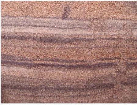
The protection of groundwater drinking supplies involves predicting the fate of contaminants in aquifers. This is a challenging and uncertain exercise using the theory of solute transport. The theory is simple for homogenous aquifers and can be verified using laboratory reduced-scale models. In nature, however, homogeneity is not common. Most often, aquifers are stratified and contain many sub-horizontal sub-layers (Fig. 1).
Figure 1 – Cleaned face, excavated beach sand (stratified aquifer), courtesy of Coline Taveau.
Stratification yields a range of values for the hydraulic conductivity, K, which can be evaluated at three scales. The small scale is that of soil samples: their quality must be assessed and their grain size distribution analyzed to check for sub-layer mixes [1, 2] before using reliable methods to predict the K values [3-5]. The middle scale is that of field permeability tests: correct methods must be used and verifications performed [6-9]. The large scale is that of pumping tests. Since large-scale tests are more likely to meet preferential flow paths, they are likely to yield larger K values than small-scale tests, which may be viewed as a scale effect. A few cases of stratified sandy aquifers were studied by Chapuis [10]. For all aquifers, the stratification led to unimodal or multimodal lognormal K distributions, which were similar at small and middle scales. The large-scale (pumping) K corresponded perfectly to the K distributions at small and middle scales. Therefore, after using a quality control of data and interpretations [11], it was concluded that there was no scale effect for K in the aquifers.
This paper examines non-reactive tracer tests in stratified aquifers, which involve the effective porosity ne, the longitudinal dispersion coefficient, DL, and dispersivity, αL. For example, the break-through curves (BTCs) of field tracer tests, which are curves of concentration C versus time t, often show early arrival, scale-dependent longitudinal dispersion, and long tails [12-14]. Hydrodynamic dispersion results mostly from the variability of the groundwater velocity field within the aquifer, and is much smaller in laboratory tests than in field tests. This would explain experimental results for αL. In addition, diffusion from the high-K layers into the low-K layers
and 3D heterogeneity may explain the longer tailing of the field BTCs.
Hydrodynamic dispersion has been investigated using theoretical and numerical studies. Dispersion is treated in statistically correlated permeability fields, which have disclosed some correlations between the aquifer heterogeneity and its dispersivity. For example, DL was found to be proportional to the correlation length of the K field and the variance of the K distribution when it is lower than one [15-17]. Numerical studies have confirmed this finding, but they need to cope with several complex issues including those specific to numerical grids, time steps, and calculations.
Hundred of theoretical papers have studied hydrodynamic dispersion but very few have given
ne values for real aquifers. In practice, ne is found to be only slightly lower than total porosity n in
homogenous soils (e.g., laboratory tracer tests), and lower than n in stratified or heterogeneous soils, but by how much? For fractured media ne may be much smaller than n [18]: for the highly
fractured limestone in the Montreal area, n is in the 3–5% range whereas tracer tests give about 0.75% for ne.
The missing research and information about ne is unfortunate for all specialists who need to predict the fate of contaminants and protect drinking water supplies. Despite academic progress, there is no predictive method for ne. Also, most field tracer test data are difficult to fit with theoretical models [19, 20]. In short, the theoretical study of dispersion is becoming more and more complex but practitioners must guess the field ne and DL values or estimate them by fitting
the BTC to a simple model. This has enlarged the gap between theoretical research and practical needs.
The objective of this paper is to develop closed-form expressions for the effective porosity and longitudinal dispersivity of the hydraulically equivalent homogeneous aquifer (HEHA) ne HEHA
and αL, HEHA, which will help to plan tracer tests and interpret their results. The closed-form
expressions must be linked to the local hydraulic properties as obtained by other common tests. They must provide the practical tools which are currently missing.
2. THE TWO PROBLEMS
The first problem in this Technical Report is natural seepage in a stratified, confined, horizontal aquifer of constant total thickness b. Its hydraulic conductivity K varies only in the vertical direction z but not with the horizontal direction x. Each sub-layer of height bj (thickness) has a
horizontal hydraulic conductivity Kj. The boundary conditions (BCs) are two constant hydraulic
heads, h1 at x1 and h2 at x2. This is a simple case of rectilinear seepage where the gradient i = (h2–
h1)/(x2–x1) is constant. The hydraulic head h depends linearly upon x:
2 1 2 1 1 2 2 1 2 1 0 x x x h x h x x x h h x h ix h ( ) , (1)
The two constants of Equation (1) are directly given by the BCs. The total flow rate Q is the sum of the flow rates Qj in each sub-layer, leading to the K composition rule:
ave j j j j j j j j bK i b K i x x h h b K Q Q
2 1 2 1 ) ( (2)The second problem is for radial steady-state: a well pumps the same aquifer at a constant flow rate Q. The perfect well is vertical and fully penetrating, centered at r = 0, and of radius rw. The BCs are two constant hydraulic heads, h1 and h2 at radial distances r1 = rw and r2 = R, with R
>> b >> rw. The rectilinear groundwater flow converges towards the well. Using the basic
equation of Thiem [21], the total flow rate Q is related to the flow rates Qj in each sub-layer by:
ave j j j j w j j j j A K b AbK r R h h b K Q Q
) / ln(( 2 1) 2 (3)in which the constant A is introduced for simplification.
Initially the non-reactive tracer concentration C is zero everywhere. Starting at time t = 0, the tracer concentration in the entering water is maintained at C0 (step function), either forever or for a limited time. It is assumed that small-scale diffusion does not play a role in the flow and transport equations. Pure convection is considered: the C0 step produces a piston flow in each sub-layer. The resulting large-scale longitudinal dispersion DL is caused only by variations in
water velocity at the sub-layer scale. Variations at the individual pore scale are not considered. The arrival time of the non-reactive tracer is used to determine the effective porosity ne, HEHA of the
hydraulically equivalent homogenous aquifer of mean hydraulic conductivity Kave.
3. CLOSED-FORM SOLUTIONS – FINITE NUMBER OF SUB-LAYERS
For the two problems defined in section 2, we consider an HEHA having the same flow rate for the same gradient, and thus a single K value equal to the Kave value for the stratified aquifer.
This is a common assumption in groundwater field and laboratory tests. This assumption of homogeneity with a mean Kave is correct only for the flow rate. For the tracer test, however, an
analytical expression must be found for the effective porosity ne, HEHA of the HEHA, which is the
first objective of this Technical Report. The second objective is to find an analytical expression for the HEHA dispersivity. The third objective is to try to better understand three characteristics of field tracer tests: (1) early arrival, (2) scale-dependent longitudinal dispersion, and (3) long tail.
3.1. Natural Seepage Case
In the counterpart HEHA, the water velocity is equal to the Darcy’s velocity divided by the equivalent effective porosity ne,HEHA. The value of arrival time t is:
, , , , ave HEHA e ave HEHA e ave HEHA e K n a K h h n x x i K n x x V x x t 1 2 2 1 2 1 2 1 2 (4)in which the constant a is used for simplification. Consider now the finite number of sub-layers of index j, for which Km ≤ Kj ≤ KM. The nej may also take different values. The indexes m and M
are used for the sub-layers having the minimum (m) and maximum (M) values of K. In the stratified aquifer, the most pervious sub-layer has a flow rate QM which contributes to a high
percentage α of the total flow rate Q, and thus: .
M m i j j M M M m i j M M b K b K Q Q Q Q (5)The tracer arrives first at time tM in the most conductive sub-layer and thus:
. M eM M K n a t (6)
The first tracer arrival gives an exit concentration C, obtained with the mixing rule as: , M Q C Q C 0 (7)
and thus the tracer first arrives at C = C0 (QM/Q), close to C0, and at a time tM. This may be
interpreted as if the aquifer was homogeneous, with some Kave value, which means that for the
field tracer test the times t and tM are confused:
. , M eM M ave HEHA e K n a t K n a t (8)
This, in turn, yields an equivalent ne, HEHA value defined as:
. , M ave eM HEHA e n KK n (9)
Since Kave is smaller than KM, Equation (9) means that ne is always smaller than the individual
neM of the most pervious sub-layer. We recall that for a homogenous material, it has been found
that ne is close to n, as in column tests [22]. Equation (9) explains why field tests in stratified
3.2. Pumping Case
In the HEHA the tracer takes a time t to travel from r = R to r = rw. During this time interval, the well has pumped a water volume Vout, which was needed to extract the volume of water Vin
moving in the pores between R and rw. This equality is expressed as:
, ) ( w e e in out Qt V n R r b Bbn V 2 2 (10)
in which the constant B is used for simplification. Using Equation (3) for the total flow rate Q, the value of arrival time t for the equivalent homogenous aquifer is:
. ave e e e K A n B K b A n b B Q n b B t (11)
Consider now the sub-layers of index j. In the stratified aquifer, the flow rate QM provided by
the most pervious sub-layer represents a high percentage α of the total flow rate Q, and thus Equation (5) applies. The first tracer arrival occurs at a time tM in the most conductive sub-layer,
obtained as: . M eM M K A n B t (12)
The tracer reaches the pumping well at concentration C obtained with the mixing rule (Equation 7), and thus at C which is close to C0, and at a time tM. This may be interpreted as if
the aquifer was homogeneous, which means that for the field tracer test the times t and tM are
confused: M eM M ave e K A n B t K A n B t . (13)
This, in turn, yields an equivalent ne value, again defined by Equation (9). Since K is smaller
than KM, Equation (9) means than the ne value (obtained with the tracer arrival in the well) is
always smaller than the neM value of the most conductive sub-layer.
3.3. Examples
(1) A stratified aquifer has a periodic layering of two types of soils (e.g., coarse sand and medium sand) such as b1 = b2 = b/2, K1 = KM = 10 K2, and also ne1 = ne2. The composition rule for K
gives: K = 0.5 K1 + 0.5 K2 = 0.55 KM and thus α = 91% and ne = 0.55 neM. As a result, if ne1 = ne2
= 38%, the tracer arrival in the pumping well corresponds to a ne value of only 21%.
(2) A stratified aquifer has a periodic layering of three types of soils (coarse gravelly sand, medium sand, and silty sand) such as b1 = 0.1b, b2 = 0.5 b, b3 = 0.4b, K1 = KM = 16 K2 =162 K3,
and ne1 = ne2 = ne3 = 40%. The composition rule for K gives: K = 0.1 K1 + 0.5 K2 + 0.4 K3 =
0.133 KM and then α = 75% and ne = 0.133 neM. As a result, the arrival of the tracer in the
pumping well corresponds to a ne value of only 5.3%. This example roughly reproduces the
stratification of our unpublished tracer test at Blainville (Quebec), for which a converging tracer test yielded a ne value close to 5%.
4. CLOSED-FORM SOLUTION – K DISTRIBUTION
For the two problems defined in section 2, involving an ideally stratified aquifer and for 0 ≤ z ≤ b, we consider firstly a lognormal and then a normal K distribution.
4.1. Lognormal K distribution
The lognormal distribution for K has the following probability density function:
2 2 2 2 1 K K K K K x z K ln ln ln ln ln , ) exp ln ; ( , (14)where μlnK and are the mean and variance of ln(K). In addition, all sub-layers are assumed to
have the same effective porosity ne. In the theory hereafter, there is no assumption concerning
spatial correlation. The water flows parallel to stratification. The velocity field depends on the
K(z) field, the constant gradient i (at all x values for the first problem, at any constant r value for
the second problem), and a constant ne. There is no dispersive movement, which would cause
mixing.
2
K
ln
The cumulative distribution function for K, here called f(K), is:
ln
erf( ) erf ) ( ln ln X K K f K K 2 1 2 1 2 2 1 2 1 , (15)in which erf is the error function, and the parameter X is defined by Equation (15). With a
lognormal distribution, the average K value, Kave, for the flowrate, is mathematically given by:
2 2 K K ave K ln ln exp . (16)
The steady state flow rate Q is given by Equations (2, 3) for the two problems defined in Section 2. A small sub-layer (Kj, ne) contributes to the exit tracer mass only after a time t*
defined using either Equation (6a) or Equation (12a) as follows: K
n a
t* e for the 1D vertical plane problem, and (6a)
K A
n B
t* e for the pumping problem. (12a)
The most conductive sub-layers are the first to supply the exit tracer mass, and the gradual input of all sub-layers produces a non-reactive tracer break-through curve (BTC). The total input to the tracer mass by all sub-layers is obtained as:
) erfc( ) ( erf ) ( erf *) ( *) ( ) , ( ) , ( X X X dr dh C dz t K b r dr dh C dz t K b r C t x C QC t x QC M m M j K K K K 2 1 2 1 2 1 2 1 2 1 1 2 2 0 0 0 0
, (17)Equation (17) can be compared with the solution of Ogata and Banks [24] to the 1D advective-dispersive equation along the x axis, for steady seepage within a column at a constant average velocity V = Ki/ne, and a constant longitudinal dispersion coefficient DL:
) , ( ) , ( ) , ( c x t x D t x c t t x c x x h K L 22 (18)
The initial and boundary conditions are C(x, 0) = 0 for x ≥ 0, C(0, t) = C0 for t ≥ 0, and C(∞, t) = 0 for t ≥ 0, where C0 is the constant injected concentration. The solution is:
t D Vt x D Vx t D Vt x C t x C L L L 2 2 1 2 2 1
0 erfc exp erfc
) ,
( (19)
The same solution was obtained using other theories, e.g., the random walk model [25]. In many cases, Equation (19) can be simplified by omitting its second term, the error being less than 3% when DL/Vx ≤ 0.0002 [24]. Equations (17) and (19) are similar except for the often small
second term of Equation (19). In this Technical Report, Equation (17) was derived assuming pure convection without diffusion. However, the field data may be viewed as resulting from dispersion, which is caused by the water velocity distribution. Equation (19) was obtained assuming a homogeneous soil in which dispersion did play a role, when the flowing water has a mean velocity value given by V = Kave i/ne. To facilitate the comparison, Equation (17) is rewritten as:
ln ( *)
erfc ln ( *) [ln ] . erfc ) , ( ln ln ln ln 2 2 2 1 2 2 1 2 0 K K ave K K K t K t K C x t C (20)In the BTC, the condition C/C0 = 0.5 is used to obtain ne, lnK for the HEHA. When C/C0 = 0.5,
the erfc function equals 1, which means that K = exp(μlnK). As a result C/C0 = 0.5 corresponds to
μlnK (K at 50%), whereas the flow rate corresponds to Kave. Then t50 lnK is lower than that which
would be calculated with the ne of individual layers, the ratio being that of exp(μlnK) and Kave. It
gives:
ave e ave K e K K K ej HEHA e n n K n KK n 2 50 2 exp( ) / exp ) exp( ln ln ln ln , , (21)in which K50 is the K value such as 50% of the K population is lower than K50. In practice, Equation (20) is calculated with the relationships between K and t* (Eqs. 6a and 12a), and then the real time t in Equation (20) is obtained as:
2 2 50 2 2 2 2 ave ave K e HEHA e K K K n n t t , exp ln * (22)Equation (21) confirms the prior finding of Equation (9): ne, HEHA (obtained with the tracer
arrival or BTH) is smaller than the single ne of the sub-layers. This also confirms the usual
observation of “early” tracer arrival in field tracer tests. In general, the values of μlnK vary between about -11 and -7 whereas the values of σlnK vary between 0 (e.g., spheres having the same diameter) and about 2. As a result, the ratio (ne, HEHA / ne) predicted by Equation (21) varies
The comparison of Equations (17) and (19) also gives the longitudinal dispersion coefficient: , ln , e ave K HEHA L LKn i D 2 2 1 (23)
and thus, because no molecular diffusion D* was considered here: .
ln ,HEHA KL L 212
(24)
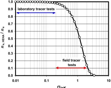
Figure 2 – Variation of the ratio (ne, HEHA / nej) predicted by Equation (21) as a function of μlnK
(from about -11 to -7) and σlnK (from about 0 to 2
0.0 0.1 0.2 0.3 0.4 0.5 0.6 0.7 0.8 0.9 1.0 0.01 0.1 1 10 lnK ne, HE HA / n e
laboratory tracer tests
field tracer tests
4.2. Normal K distribution
We now consider the two problems for the case of a normal K distribution, with a mean μK and
a standard deviation σK. The theoretical development provides:
. , , n and L n K K HEHA L e HEHA e 2 2 2 1 (25)
These results can also be deduced from the classical solution [26], which means that if the K distribution is normal, then ne, HEHA is equal to the single ne within individual sub-layers. However,
a field tracer test gives a ne HEHA value that may be much lower than the ne value within individual
sub-layers. This implies that the interpretation of field tests should assume a lognormal K distribution, which seems to be the usual finding with either small or middle scale K values [2, 9-10]. According to these results, the longitudinal dispersivity αL, HEHA is proportional to the
5. APPLICATIONS 5.1. Laboratory tests
Consider a 1D laboratory tracer test. Uniform sand was poured between two parallel, one meter long clear walls. The sand was compacted as regularly as possible, for example in small layers about 2.5 cm high, using a tamper of defined weight and height of fall. At the end of the process, despite all precaution, the sand layers still have a small variation in K. We must estimate first the K distribution and its variance, and then the resulting dispersivity according to the proposed equations.
The sand is defined by its grain size distribution curve (GSDC) and the roundness factor, RF, of its particles. The minimum and maximum values for the porosity n, nmin and nmax, or the void ratio e, emin and emax, can be determined using standard tests [27, 28] or with the chart of Youd [29]. This chart was transformed into equations linking emax and emin to the sand coefficient of uniformity CU and RF [8]. Some variability in GSDC and compaction method yields some variability for the effective diameter d10 and void ratio e, which can be used to assess the K value. Assume for example that d10 varies between 0.14 and 0.18 mm, thus d10 = 0.16 ± 0.2 mm, and that e varies between 0.46 and 0.58, thus e = 0.52 ± 0.06.
Many equations can be used to predict K. The assessment of the performance of 45 methods [5] lead to the conclusion that the most reliable for natural non-plastic soils are that of Chapuis [4], followed by that of Hazen [30] coupled with Taylor [31], and that of Kozeny-Carman [3]. Here, we employ the predictive Equation (26) which predicts K values between half and twice the experimental K values for tests avoiding all of the common 14 mistakes of laboratory tests [5]:
7825 0 3 2 10 1 4622 2 . . ) / ( e e d s cm K . (26)
Equation (26), where the effective size d10 is in mm, gives a K value of 2.17 x 10⁻² cm/s when
the mean values for d10 and e are considered. Using for simplification a = 2.4622, b = 0.7825, d10 = x and the void ratio e, the logarithmic differential of Equation (26) is:
x dx e e de e de b e e d x dx e de b K dK 2 1 2 3 1 1 2 3 ) ( ) ( . (27)
Equation (27) is then used to assess the relative error (dK/K) resulting from the relative errors on d10 (dx/x) and e (de/e) when these values are small (≤ 10%), and also the relative uncertainty
(ΔK/K), where ΔK is the absolute value of dK. The equation for relative uncertainties is: x x e e e e e b K K 2 1 2 3 ) ( . (28)
The numerical application for the previous sand data yields: 44 0 16 0 02 0 2 52 1 52 0 06 0 52 0 2 06 0 3 7825 0 . . . . . ) . . ( ) . ( . K K . (29)
As a result, K = (2.2 ± 1) x 10–2 cm/s. However, since the variation exceeds 20%, it is better to
use the direct calculation that gives: 1.36 x 10⁻² ≤ K ≤ 3.27 x 10⁻² cm/s. Similar developments
can be made with the Hazen-Taylor and the Kozeny-Carman equations.
We now consider the normal and lognormal K distributions corresponding to the K range, as shown in Fig. 3: with μK = 2.172 x 10⁻⁴ m/s and σK = 4 x 10⁻⁵ m/s, Equation (25) gives αL = 5.75
x 10–4 m = 0.6 mm; with μlnK = -8.435 and σlnK = 0.180, Equation (24) gives αL = 2.3 x 10⁻⁴ m =
0.23 mm. Such small values are regularly observed in laboratory tracer tests. They are also observed in field tracer tests in individual layers [32-33]. The ne, HEHA value is predicted by
Equation (21) for the lognormal K distribution: the factor is 0.984, and thus ne, HEHA = 98.4% n for
homogeneous sand. In practice, the laboratory tracer tests regularly yield ne slightly smaller than
n for sand, or for clay [34], consistent with the lognormal assumption.
Figure 3 – The K range for the example of a laboratory tracer test can be fitted with normal and with lognormal K distributions which are very close, in this case.
0% 10% 20% 30% 40% 50% 60% 70% 80% 90% 100% 1.E-04 1.E-03 x = K (m/s) % c ases lo w er th an x mean min max normal dist lognormal dist.
Consider now a poorly prepared test in which the sand has variations in d10 and e due to poor control of gradation and compaction. This may double the previous standard deviations, and thus multiply by 4 the variances. As a result, the test provides αL values of 2.4 mm for a normal K
distribution and 1 mm for a lognormal K distribution, whereas the ratio of Eq. (21) is 0.937, thus
ne, HEHA equals 93.7% of the average n value. Since the n value was poorly controlled during the
sand placement, and thus is poorly known, the exact difference between n and ne is poorly known, and thus one cannot distinguish a well-prepared from a poorly-prepared laboratory tracer test.
According to previous calculations, a lognormal K distribution gives a very small αL, as
regularly obtained with laboratory test data, and a ne value slightly smaller than the sand mean n value, also as regularly obtained with the laboratory test data. However, the differences resulting from the two assumed K distributions, normal or lognormal, are too small to tell which distribution should be preferred.
5.2. Field pumping tests
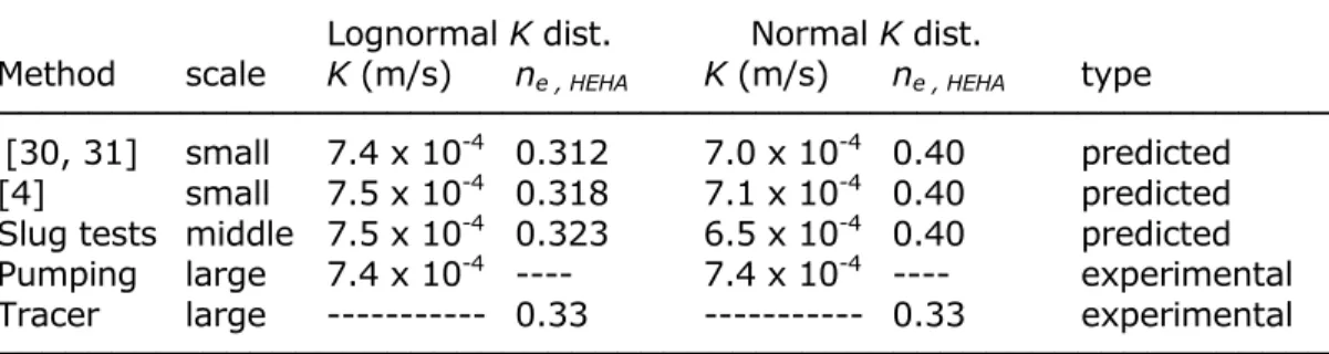
Consider the sand aquifer at Lachenaie (Quebec). Converging tracer tests were performed after steady-state seepage for a constant flow rate pumping test was reached. According to the tracer test data, ne = 33%, whereas n was close to 40%. The field value for ne can be compared here to that derived using the new equations of this Report and the experimental K distributions at small scale (samples) and middle scale (field tests in MWs) presented elsewhere [35–37].
Using the grain size distributions and the porosity, the small-scale K values were predicted using the methods of Hazen-Taylor [4, 30-31] and Chapuis [4]. Each small scale K distribution was fitted with lognormal and normal distributions, which gave the predicted large-scale K and
ne, HEHA for the hydraulically equivalent homogenous aquifer. The results appear in Table 1. The
middle-scale field K values (slug tests in developed monitoring wells) were also adjusted with lognormal and normal distributions (Fig. 4), which gave the predicted large-scale K and ne, HEHA.
All results (Table 1) show that the new equations for a lognormal distribution better predict the large-scale K and ne, HEHA than the normal distribution. However, the differences are small because
the variances are small for this fairly homogenous sand aquifer.
Figure 4 – Experimental K distributions for the Lachenaie sand aquifer, with the lognormal and normal best fits for the slug tests in monitoring wells (MWs) after development.
0% 10% 20% 30% 40% 50% 60% 70% 80% 90% 100%
1.E-03 1.E-02 1.E-01 1.E+00
x = K (cm/s) % of cases lo w er th an x pred. K (samples) K tests in MWs lognormal fit MWs normal fit MWs data pumping
Table 1. Comparison of predicted and experimental values for large-scale K and n, HEHA.
────────────────────────────────────────────────────────── Lognormal K dist. Normal K dist.
Method scale K (m/s) ne , HEHA K (m/s) ne , HEHA type
────────────────────────────────────────────────────────── [30, 31] small 7.4 x 10⁻⁴ 0.312 7.0 x 10⁻⁴ 0.40 predicted
[4] small 7.5 x 10⁻⁴ 0.318 7.1 x 10⁻⁴ 0.40 predicted
Slug tests middle 7.5 x 10⁻⁴ 0.323 6.5 x 10⁻⁴ 0.40 predicted
Pumping large 7.4 x 10⁻⁴ ---- 7.4 x 10⁻⁴ ---- experimental
Tracer large --- 0.33 --- 0.33 experimental ──────────────────────────────────────────────────────────
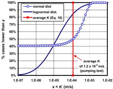
Let us examine now a less homogenous, stratified, sand aquifer (Blainville, Quebec), for which a converging tracer test was performed after reaching steady-state pumping conditions. Unfortunately, there were too few tests to assess the K distributions at middle scale (3 field tests in 3 MWs) and small scale (3 GSDCs for 3 composite samples). However, a trench revealed that the nearly horizontal sub-layers were 1 to 5 cm thick, and varied from pea gravel to silt, which means that K varied roughly from 10-7 to 10-3 m/s. The other data were: Kave = 1.2 x 10⁻⁴ m/s (pumping test), ne, HEHA = 5% (field tracer test), and n = 40% for each sub-layer. A lognormal K
distribution was found which explains the Kave value, the estimated K range and the ne, HEHAvalue
(Figure 5): it has a mean μlnK of -11.107 and a standard deviation σlnK of 2.039, for which Equations (16) and (21) yield Kave = 1.2 x 10⁻⁴ m/s and ne, HEHA= 5% and also a K range similar to
that field estimated. For comparison, a normal K distribution with the same Kave strongly differs from the lognormal distribution (Figure 5), and it predicts that ne, HEHA= 0.40 as for the individual
sub-layers, a much too high value which would not fit the field test value of 5%.
Figure 5 – Blainville field tracer test (steady-state pumping): the normal and lognormal K distributions which fit the average Kave are quite different. The lognormal K distribution is the
only one that also fits the K range and the ne,field of 5% given by the tracer test.
0% 10% 20% 30% 40% 50% 60% 70% 80% 90% 100%
1.E-07 1.E-06 1.E-05 1.E-04 1.E-03 1.E-02
x = K (m/s) % c ases lo w er th an x normal dist lognormal dist. average K (Eq. 16) average K of 1.2 x 10⁻⁴ m/s (pumping test)
5.3. Collected data for αL
The new predictive Equation (24) for the longitudinal dispersivity αL is compared here to the
αL values obtained using field data and collected by Gelhar et al. (1992) [14]. Figure 6 presents
the predicted and collected αL values versus the scale (length) of the problem, which has been the topic of many papers. In the log-log plot of Figure 6, the predicted αL values correspond to a
straight line for a constant value of σlnK. In general, the values of μlnK vary between about -11 and -7 whereas the values of σlnK vary between 0 (e.g., spheres having the same diameter) and about 2. Values of σlnK of 0.05, 0.1, 0.2, 0.5, 1, and 2 are used in Figure 6, where it appears that all field data could be simply due to lognormal K distributions. However, we do not suggest that the μlnK
and σlnK values for the tested aquifer could be surmised from the tracer test data. The field αL values were obtained using different theories and numerical models, and in many cases the 1D advective-dispersive uniform flow solution even though most field problems were 2D or 3D. As a result, most αL values are considered to have a low reliability [14]. Also, those performing field studies did not always recognize the role of uncontrolled or poorly defined tracer inputs. In addition, the local values of concentration C were obtained with groundwater samples taken in monitoring wells (MWs): these are now known to depend upon the sampling protocol, the sub-layers intercepted by the MW screen and filter pack, and may also vary greatly with time for unconfined aquifers.
Figure 6 – Predicted values for the longitudinal dispersivity (Eq. 23) and comparison with the collected field data of Gelhar et al. [14].
1.E-03 1.E-02 1.E-01 1.E+00 1.E+01 1.E+02 1.E+03 1.E+04 1.E+05
1.E+00 1.E+01 1.E+02 1.E+03 1.E+04 1.E+05
scale or distance x (m) long itudi nal di sper si vi ty ( m )
Theory in this paper Gelhar et al. (1992) (lnK ) 2 1 0.5 0.2 0.1 0.05
6. NUMERICAL VERIFICATION OF THE NEW CLOSED-FORM SOLUTIONS
The new solutions for ne, HEHA and αL are valid for stratified aquifers with lognormal K
distribution, but without dispersion, assuming a plug flow in each sub-layer. These solutions can be verified first with a spreadsheet, using first an aquifer comprised of 10, 20, 40 or 100 layers, and then the closed-form solution, to assess the transition between the two representations.
6.1. Verification with a spreadsheet
Consider 1D seepage in a 200-m long aquifer, with a constant gradient of 0.01, μlnK = -8, σlnK = 0.7 (thus Kave = 4.286 x 10⁻⁴ m/s), and n = 38% for each sub-layer. The new equations predict ne, HEHA= 29.7%, and DL = 5.5 x 10⁻⁴ m2/s. Sets of 10, 20, 40 and 100 sub-layers have been used
to see how these approximations define the break-through curve. A set of forty sub-layers is enough to closely fit the closed-form solution for the lognormal K distribution (Figure 7).
Figure 7 – Comparison of break-through curves for a lognormal K distribution without dispersion, and the hydraulically equivalent homogenous aquifer (HEHA). The K distribution is approximated by 10-20-40-100 sub-layers, and the theoretical curve is given by the closed-form
solution. The (C/C0 = 50%) value occurs at an earlier time than that of the plug flow in the HEHA, which means that ne, HEHA is lower than the ne of individual sub-layers.
0% 10% 20% 30% 40% 50% 60% 70% 80% 90% 100%
1.E+06 1.E+07 1.E+08
elapsed time t (s) exi t C / C0 HEHA 10K-LN 20K-LN 40K-LN 100K-LN Theory
plug flow (HEHA)
ne of sub-layers
stratified lognormal aquifer
ne, HEHA < ne (sub-layers)
Equation (19) for 1D advection-dispersion implies a normal (not lognormal) velocity distribution. A simplified form [26] is frequently used for field data, using the three values of time for ratios C/C0 of 15.9%, 84.1% and 50% to calculate ne, σ and DL. If it is used to interpret
the data in Figure 7, it yields inexact values because the data are for a lognormal distribution. It yields σlnK = 0.752, ne, HEHA = 29.4%, and DL = 6.4 x 10⁻⁴ m2/s. The deduced values are
nonetheless close to the correct ones (lognormal K distribution) because for the case of Figure 7 the standard deviation is below unity.
However, the BTC for a lognormal K distribution without dispersion has some distortion when compared to the BTC of the HEHA with an equivalent DL as shown in Figure 7. In particular, the (C/C0 = 50%) value occurs at an earlier time, which may be interpreted also as a homogenous aquifer with a ne, HEHA lower than the ne of each sub-layer and some longitudinal dispersivity.
To complete the verifications, an example is presented for a stratified aquifer of length L = 10 m with a lognormal K distribution of mean μlnK = -8, and standard deviation σlnK = 0.1 (to
approach a plug flow in a homogenous material), 0.3, 0.7 and 1.5. T he break-through curves are given for the output at abscissa x = L = 10 m. Figure 8 shows the closed-form solution for a continuous input at concentration C0, whereas Figure 9 is for an input C0 during a time interval Δt = 120 s. The closed-form for this case is obtained using the superposition method with Equation (20), which gives:
2 2 1 2 2 1 0 K K K K K t t t K C t x t C ln ln ln ln erfc ln ( * *) *) ( ln erfc ) , , ( , (30)Figure 8 – Comparison of theoretical break-through curves for lognormal K distributions with the same mean but different standard deviations. For a continuous injection at concentration C0, an
increased σlnK produces an earlier arrival of the tracer, with more curve distortion.
0% 10% 20% 30% 40% 50% 60% 70% 80% 90% 100%
1.E+04 1.E+05 1.E+06 1.E+07
time t (s) C/ C0 = - 8.0 = 0.1 = - 8.0 = 0.7 = - 8.0 = 1.5 continuous injection L = 10 m, ne = 0.35 gradient = 0.01 = - 8.0 = 0.3
It appears that an increased σlnK produces an earlier arrival of the tracer, more curve distortion,
and also a longer tail (Figure 9). All these features are typical of field tracer tests. Therefore the new closed form-solutions for a stratified aquifer and a lognormal K distribution predict realistic values for the resulting effective porosity, ne, HEHA, and the shape of the break-through curve.
Figure 9 – Comparison of break-through curves for lognormal K distributions with the same mean but different standard deviations. For a continuous injection at concentration C0, an
increased σlnK produces an earlier arrival tracer, more curve distortion, and also a longer tail.
0.E+00 1.E-04 2.E-04 3.E-04 4.E-04 5.E-04 0 500000 1000000 1500000 time t (s) C/ C0 = - 8.0 = 0.1 = - 8.0 = 0.3 = - 8.0 = 0.7 = - 8.0 = 1.5
6.2. Verification with a finite element method
Even with a set of forty sub-layers to represent the lognormal K distribution, the verification of the new equations with a finite element code cannot be rigorous. This happens because the code uses the advective-dispersive equation and cannot take the input αL = 0 as assumed in the new equations. The following paragraphs explain why a verification of the new equations with a finite element code cannot be a real proof. The code can solve the particle tracking problem, which is a case where αL = 0. Unfortunately the particle tracking does not give the masses of non-reactive contaminant and the resulting concentrations, which are needed to verify the new equations.
A numerical solution with αL > 0 contains some numerical dispersion and oscillation. Numerical dispersion spreads out a tracer more than predicted by analytical solutions. Numerical oscillation produces local concentrations that are higher than 100% or negative. T o achieve correct numerical results with minimal numerical dispersion and oscillation, the finite element size and the time steps must respect two criteria, for the Peclet Number (PN ≤ 2) and the Courant
Number (CN ≤ 1).
To try to verify numerically the new equations, with αL = 0, one may try to adopt a very low
αL value. This creates numerical problems, because the PN constraint requires using finite
elements of very small size, which increases the number of nodes and equations to be solved. Consider the definition of PNx for the x direction, where Δx is the nodal x-spacing and Vx the x
component of velocity, and the case here without molecular diffusion, D* = 0: 2 L x L x L x Nx VD x VV xD x P * . (31)
For a 1D case, taking 10-3 m for α
L means that the finite elements must not exceed 2 mm in the
x direction. In addition, the numerical code needs a transverse dispersivity αT, which is usually
taken as 0.1αL, thus 10-4 m in the example. According to Equation (30) the finite elements must
not exceed 0.2 mm in the z direction. The maximum size for the finite elements is then 2 mm x 0.2 mm, which means an aspect ratio of 10, higher than the recommended value of 2 or 3. However, since this is a 1D problem, fully saturated, an aspect ratio of 10 can still give a good numerical solution. As a result, for a 1-m long problem, the grid has rows of 500 elements and columns of 40 elements if a single element is used per sub-layer, but this is known to give a poor numerical solution. A rule of thumb is to use a minimum of 8 elements per sub-layer, which is rarely done in groundwater studies, but is well documented in finite element theory. The coarser grid has thus 500 x 40 x 8 = 160 000 elements, and is borderline to good accuracy, which should be checked using detailed convergence analyses of type h- and p- , which unfortunately are rarely done in groundwater studies.
Let us now examine the conditions for the Courant number, CN:
1 x t V CNx x . (32)
Assume for example Vx = 1 x 10⁻⁵ m/s, whereas Δx must not exceed 2 mm. It means that the
time step Δt must be smaller than 200 s. However, field conditions are rather for K values in the order of 10-4 m/s and field gradients in the order of 10-3 (one m per km), which yields velocities
in the order of 10-6 to 10-7 m/s, and thus the time step must be smaller than 20 or 2 s. Since a field tracer test lasts days, weeks, or months, the finite element calculation requires a very large number of time steps to cover the test duration.
Despite the limitations inherent to finite elements, a partial verification is presented for a low
αL value. A first model gives the BTC for the HEHA, with a low αL, while a second model gives
the BTC for the stratified aquifer with a lognormal K distribution and the same low αL. A finite
element code [38] was chosen, which was previously proven to be reliable in a study assessing the performance of numerical codes for both saturated and unsaturated seepage [39]. In this code, the user can define and use a special finite element, having special properties, to realistically reproduce the hydraulic behavior of pipes or reservoirs, which facilitates the handling of complex boundary conditions linking the hydraulic head and its partial derivatives [40]. In the case of pumping tests, the code provides results identical to theoretical solutions [37]. For unconfined aquifers, the code also gives the seepage face in the well screen [41]. The code was used to solve many problems involving unsaturated and saturated seepage [42, 43].
The result of a finite element calculation appears in Figure 10 for a 2D plane tracer test in an aquifer 1 m long. The lognormal K distribution has a mean of -8.5 and a standard deviation of 0.3. The stratified aquifer is represented by 10 or 20 layers. Each layer has the same ne of 0.40. The numerical code does not accept αL = 0, and thus is given values of 0.01 and 0.001 for αL and
αT respectively. The numerical BTC for the HEHA is nearly symmetrical because the variance is
small. The numerical BTC for the lognormal K distribution is distorted, with an early arrival, and a much longer tail (Figure 10). This corresponds, roughly, to the closed-form solution.
Figure 10 – Numerical models to compare the break-through curves for the HEHA with some dispersion and the stratified aquifer with a lognormal K distribution plus the same dispersion as the HEHA. The lognormal K distribution is approximated by either 10 or 20 homogenous sub-layers. The (C/C0 = 50%) value occurs at an earlier time, which means that ne, HEHA is lower than
ne, and there is more dispersivity with a longer tail.
0.0 0.2 0.4 0.6 0.8 1.0 1.2 1.4 1.6 1.8 2.0 0 3600 7200 10800 14400 18000 elapsed time t (s) m ass flux / Q HEHA - 1 ave. K logN-10K-P2C0.3 logN-20K-P2C0.3 long tail close to symmetry, no long tail earlier arrival thus lower ne
7. DISCUSSION
The main goal of this Technical Report has been to establish new analytical solutions for the effective porosity and break-through curves in stratified aquifers having a lognormal K distribution, under plane flow in a vertical section, or radial flow (pumping well). Stratified models have been widely used, since they provide a useful conceptual framework of transport in aquifers consisting of layered geological bodies. A rapid search of publications revealed that the “web of science” listed 224 papers on the topic [“Tracer test” aquifer dispers*] where dispers* includes dispersivity and dispersion, but only 14 papers on the topic [“Tracer test” aquifer, “effective porosity”].
The missing information about ne is unfortunate for all specialists who need to predict the fate of contaminants and protect drinking water supplies. Despite scholarly progress, there has not been any predictive method for ne, and thus, there has been a gap between theoretical research and field needs. We have presented a predictive method for the effective porosity and the dispersivity of stratified aquifers, when their K distribution is lognormal, as frequently observed.
Field tracer tests are known to be highly influenced by stratification, which may explain early tracer arrivals, increasing values of dispersivity with distance, and the long tail of the break-through curves. When the flow path length increases, the tracer encounters velocities with increased variability, which leads to what is currently presented as a scale effect of dispersion. Various upscaling methods were proposed for dispersion but few methods have taken the real stratification and heterogeneity into account.
Our previous studies have shown that in many aquifers a detailed analysis of small-, middle- and large-scale K values indicates that there is no real scale effect for K. The small- and middle-scale K values follow similar lognormal distributions, which statistically explain the large-scale K values of pumping tests. Here, we have found that a lognormal K distribution can fully explain:
(1) the early arrival of the tracer in field tests, using an equation providing the ne value for the hydraulically equivalent homogenous aquifer (HEHA);
(2) the increase of αL, with distance and also with the variance of lognormal K
distribution; the equations obtained have the capacity to explain all previous field and laboratory results, which had been attributed to some scale effect; and
(3) the long tail of field break-through curves, which was shown here to be related to the variance of the lognormal K distribution.
In short, the equations presented above simply confirm that the supposed scale effects for K or αL are not genuine scale effects in the sense of physics [44].
Closed-form solutions for stratified aquifers are useful for analyzing rapidly a situation; they are valuable tools for investigating transport and dispersion in natural aquifers. They make it easy for users to grasp a problem using easy-to-obtain continuous graphs instead of having to create a numerical model, perform parametric studies to assess the h– and p– convergences and tabulate results, which is time-consuming. Obtaining a closed-form solution, however, usually requires a few simplifying assumptions which may reduce the realism of the solution. Checking whether the closed form is realistic may be done in numerical studies, which do not make any of the simplifying assumptions. However, as shown, the numerical codes cannot accept the input αL
= 0 for individual sub-layers as assumed in the new equations of this Technical Report, and they have limitations.
8. CONCLUSION
We have analyzed stratified aquifers in which the hydraulic conductivity K has a lognormal distribution. Closed-form solutions are obtained for two seepage cases, in a vertical plane, and towards a pumping well. For each case, solutions are provided for a finite number of sub-layers, to help the reader to grasp basic findings, and then, for a lognormal K distribution. The comparison between a stratified case and the hydraulically equivalent homogenous aquifer (HEHA) yields equations for the effective porosity ne, HEHA and the longitudinal dispersivity DL, HEHA of the stratified aquifer.
It is shown that ne, HEHA is smaller than the individual ne of the sub-layers. If the K distribution
is lognormal, ne, HEHA and ne are related by an equation using the mean and variance of ln(K). For
laboratory experiments with homogenized soils, placed and compacted layer after layer, the resulting variability in K is shown to be low. The theory predicts that the large scale ne, HEHA is
very close to ne and thus almost equal to n, as frequently observed in laboratory experiments. For a lognormal K distribution, the break-through curve (BTC) equation is shown to be similar to the classical 1D advection-dispersion equation. When the variance of ln(K) is low ( ),
the assumptions of normal or lognormal distributions when analyzing the BTC yield results which are close. The closed-form equation for the longitudinal dispersivity depends on the variance of ln(K) and the distance traveled. The BTC for a short-duration injection is
automatically asymmetric with early arrival and a long tail, as usually found in field tracer tests. 1 2
K ln
Even if many previous publications have examined stratified flow, none has developed the form solutions that are presented here. We have also presented a verification of closed-form solutions using a spreadsheet, and using the finite element method. As previously explained, the latter has some problems due to its inability to accept the input αL = 0 for sub-layers as assumed in the new equations of this Technical Report, and also to its need for a very detailed grid even for a simple case of regular stratification, due to the constraints of the Peclet number.
Field tracer experiments or pollution cases are more complex than the two problems solved here. The field dispersion depends not only upon the aquifer heterogeneity but also upon less simple geometric conditions and more complex time-variable boundary conditions. Many of the aquifer heterogeneities may be difficult to recognize and quantify. The new findings presented here help us to understand early tracer arrivals, distortion of break-through curves and long tails of BTCs. However, real progress in this research area will require collaboration between different disciplines such as sedimentology, groundwater, geotechnical engineering, geophysics, and numerical modeling, in order to better solve the problems of stratified, heterogeneous, aquifers.
9. ACKNOWLEDGMENTS
This Report results from a research subsidized by the Natural Sciences and Engineering Research Council of Canada (NSERC) to improve the quality of groundwater parameters.
10. REFERENCES
1. Chapuis RP, Dallaire V, Saucier A. Getting information from modal decomposition of grain size distribution curves. Geotechnical Testing Journal 2014; 37(2):282–295.
2. Chapuis RP. Evaluating the hydraulic conductivity at three scales for an unconfined and stratified alluvial aquifer. Bulletin of Engineering Geology and the Environment, 2015; submitted.
3. Chapuis RP. Aubertin M. On the use of the Kozeny–Carman equation to predict the hydraulic conductivity of a soil. Canadian Geotechnical Journal 2003; 40(3):616–628. 4. Chapuis RP. Predicting the saturated hydraulic conductivity of sand and gravel using
effective diameter and void ratio. Canadian Geotechnical Journal 2004; 41(5):787–795. 5. Chapuis RP. Predicting the saturated hydraulic conductivity of soils: a review. Bulletin of
Engineering Geology and the Environment, 2012; 71(3):401–434.
6. Chapuis RP. Overdamped slug test in monitoring wells: review of interpretation methods with mathematical, physical and numerical analysis of storativity influence. Canadian
Geotechnical Journal 1998; 35(5):697–719.
7. Baptiste N, Chapuis RP. What maximum permeability can be measured with a monitoring well? Engineering Geology 2015; 184:111–118.
8. Chapuis RP. Estimating the in situ porosity of sandy soils sampled in boreholes.
Engineering Geology 2012; 141–142:57–64.
9. Chapuis RP. Evaluating the hydraulic conductivity of an unconfined sand-and-gravel aquifer with permeability (slug) tests in monitoring wells. Bulletin of Engineering Geology
and the Environment, 2015; submitted.
10. Chapuis RP. Permeability scale effects in sandy aquifers: a few case studies. Proceedings
of the 18th International Conference on Soil Mechanics and Foundation Engineering,
Paris, France, 2013; 505–510.
11. Chapuis RP. Controlling the quality of groundwater parameters: some examples.
Canadian Geotechnical Journal 1995;32(1):172–177.
12. Lallemand-Barrès A, Peaudecerf P. Recherche des relations entre les valeurs mesurées de la dispersivité macro-scopique d’un milieu aquifère, ses autres caractéristiques, et les conditions de mesure. Bulletin du BRGM 2e série 1978; 3(4):277–284.
13. Anderson MP. Hydrogeologic facies models to delineate large-scale trends in glacial and glaciofluvial sediments. Geological Society of America Bulletin 1989; 101:501–511. 14. Gelhar LW, Welty C, Rehfeldt KR. A critical review of data on field-scale dispersion in
aquifers. Water Resources Research 1992; 28(7):1955–1974.
15. Gelhar LW, Axness CL. Three-dimensional stochastic analysis of macrodispersion in aquifers. Water Resources Research 1984; 19(1):161–180.
16. Schwarze H, Jaekel U, Vereecken H. Estimation of macrodispersion by different approximation methods for flow and transport in randomly heterogeneous media.
Transport in Porous Media 2001; 43:265–287.
17. Dentz M, Le Borgne T, Englert A, Bileljic B. Mixing, spreading and reaction in heterogeneous media: A brief review. Journal of Contaminant Hydrology 2011; 120– 121(SI):1–17.
18. Worthington SRH, Smart CC, Ruland W. Effective porosity of a carbonate aquifer with bacterial contamination: Walkerton, Ontario, Canada. Journal of Hydrology 2012; 464-465:517–527.
19. Fernandez-Garcia D, Rajaram H, Illangasekare TH. Assessment of the predictive capabilities of stochastic theories in a three-dimensional laboratory test aquifer: Effective hydraulic conductivity and temporal moments of breakthrough curves. Water Resources
Research 2005; 41:W04002.
20. Pedretti D, Fiori A. Travel time distributions under convergent radial flow in heterogeneous formations: insight from the analytical solution of a stratified model.
21. Thiem G. Hydrologische Methoden. Gebhardt, Leipzig, 1906; 56p.
22. Hudak PF. Effective porosity of unconsolidated sand: Estimation and impact on capture zone geometry. Environmental Geology 1994; 24:140–143.
23. Stephens DB, Hsu KC, Prieksat MA, Ankeny MD, Blandford N, Roth TL, Kelsey JA. A comparison of estimated and calculated effective porosity. Hydrogeology1998; 6:156– 165.
24. Ogata A, Banks RB. A solution to the differential equation of longitudinal dispersion in porous media. US Geological Survey Professional Paper 1961; 411–A, 13 p.
25. Fleurant C, van der Lee J. Stochastic modelling of tracer transport in three dimensions.
Proceedings of the TraM’2000 Conference, 2000; IAHS Publ. no.262, 109–114.
26. Bear J. Dynamics of Fluids in Porous Media. American Elsevier, New York 1972.
27. ASTM. Test methods for maximum index density and unit weight of soils using a vibratory table (D4253). Annual CDs of Standards, vol. 04.08, ASTM International, West
Conshohocken, PA.
28. ASTM. Test methods for minimum index density of soils and calculation of relative density (D4254). Annual CDs of Standards, vol. 04.08, ASTM International, West
Conshohocken, PA.
29. Youd TL. Factors controlling maximum and minimum densities of sands. ASTM Philadelphia, PA, Selig ET, Ladd RS (eds), 1973; STP 523, pp. 98–112.
30. Hazen A. Some physical properties of sand and gravel, with special reference to their use in filtration. Massachusetts State Board of Health, 24th annual report, Boston, 1892; pp. 539–556.
31. Taylor DW Fundamentals of soil mechanics. John Wiley & Sons, New York 1948.
32. Pickens JF, Grisak GE. Scale-dependent dispersion in a stratified granular aquifer. Water
Resources Research 1981; 17: 1191–1211.
33. Moltynaer, GL, Killey, RWD. Twin Lake Tracer tests: longitudinal dispersion. Water
Resources Research 1988; 24: 1613–1627.
34. Sevee JE. Effective porosity measurement of a marine clay. Journal of Environmental
Engineering, ASCE 2010; 136(7):674–681.
35. Gloaguen E, Chouteau M, Marcotte D, Chapuis R. Estimation of hydraulic conductivity of an unconfined aquifer using cokriging of GPR and hydrostratigraphic data. Journal of
Applied Geophysics 2001; 47(2):135–152.
36. Chapuis RP, Chenaf D, Acevedo N, Marcotte D, Chouteau M. Unusual drawdown curves for a pumping test in an unconfined aquifer at Lachenaie, Quebec: Field data and
numerical modeling. Canadian Geotechnical Journal 2005: 42:1133–1144.
37. Chapuis RP, Dallaire V, Marcotte D, Chouteau M, Acevedo N, Gagnon F. Evaluating the hydraulic conductivity at three different scales within an unconfined aquifer at Lachenaie, Quebec. Canadian Geotechnical Journal 2005; 42:1212–1220.
38. Geo-Slope. Seepage Modeling with Seep/W. Geo-Slope International, Calgary 2007. 39. Chapuis RP, Chenaf D, Bussière B, Aubertin M, Crespo R. A user's approach to assess
numerical codes for saturated and unsaturated seepage conditions. Canadian Geotechnical
Journal 2001; 38(5):1113–1126.
40. Chapuis RP. Numerical modeling of reservoirs or pipes in groundwater seepage.
Computers and Geotechnics 2009; 36: 895–901.
41. Chenaf D, Chapuis RP. Seepage face height, water table position, and well efficiency for steady state. Ground Water 2007; 45:168–177
42. Chesnaux R, Molson JW, Chapuis RP. An analytical solution for ground water transit time through unconfined aquifers. Ground Water 2005; 43:511–517
43. Chesnaux R, Chapuis RP, Molson JW. A new method to characterize hydraulic short-circuits in defective borehole seals. Ground Water 2006; 44:676–681.
44. Panfilov M. Macroscalemodels of flow through highly heterogeneous porous media.