A validation process for CFD use in building physics.

1

A validation process for CFD use in building physics.

Université de Liège, Belgium 2

Université catholique de Louvain, Belgium

*

Corresponding email: mbarbason@ulg.ac.be

ABSTRACT

Due to growing interests in environmental and building energy performance concerns, building physics simulations - and especially Computational Fluid Dynamics (CFD) – are more and more used. Unfortunately, until now, there is no clearly defined method to validate the use of these models by building engineers. This paper describes a validation process of CFD tools dealing with physical phenomena occurring in building physics. The comparison between experimental data and numerical results proves the validity of CFD use and its specific contribution to building physics modelling in comparison with thermal multizonal models. Thanks to this validation process, building engineers can improve their CFD simulations performance and their comprehension of building physics.

KEYWORDS

Building Physics Simulations, CFD, Multizone Simulations, Modelling, Validation.

INTRODUCTION

As a large part of energy consumptions is due to buildings (heating, ventilation, etc.) and because environmental concerns grow, scientists are urged to develop new tools for architects and building engineers. Thanks to growing computer capacities, new solutions are now available. Computational Fluid Dynamics (CFD) is in gestation for decades (Chen and Jiang, 1992). It has first been developed for aerospace applications but it is now getting mature for building physics. CFD permits to get a very precise description of airflows in buildings. There is no doubt that it will permit to improve Heating, Ventilation and Air-Conditioning (HVAC) systems efficiency and Internal Air Quality (IAQ).

Unfortunately, there is no clearly defined method to validate the use of CFD simulations by non-expert users. The main problem is that building physics involve lots of physical phenomena (natural or mechanical convection, radiation, etc.). For this reason, a validation process was created to guide building engineers in their learning of these tools. This validation process is established in the frame of an EDRF project called SIMBA. The aim of this project is to validate various CFD simulation tools, and to confront CFD and multizonal approaches.

METHODS

This validation method of CFD simulations is based on the possibility for new CFD users to compare their simulation results with experimental and numerical results of some typical applications in building physics. Two main axes were identified to create a complete validation process of CFD: 1) physical phenomena encountered are numerous and require different approaches and, 2) building physics applications involve various space scales.

In the first theme, four different cases were identified to cover most classical engineering cases. The first one is simply a mechanical ventilation case. The second case permits to get

2

used to free float case (thermal loads create and keep natural convection going) while the third one deals with natural ventilation case. Eventually, the fourth one approaches radiation devices (cooling ceiling and floor heating). In the second theme, once again, the approach has been separated in four steps. The first scale is a single-room. The second one is a group of partitioned rooms. The third one is an atrium exposed to solar radiation. The fourth is a complete building with open floors and a central atrium.

The two themes define sixteen different cases in a double entry array. A validation process based on 16 different cases should be too long. Moreover, it would be difficult to find complete experimental results for each case. So it is proposed to resolve one complete column and one complete line (Table 1). After having completed this validation process, it is clear that the operator will have a good knowledge of building physics simulations.

Table 1. Validation process diagram.

Single Room Partitioned Rooms Atrium Complete building Mechanical Ventilation Free Float Natural Ventilation Radiation Case 1 Case 2 Case 3 Case 4

Case 5 Case 6 Case 7

In this paper, only the first column will be discussed. The proposed line will be described in a further paper. Note that the single room column and the mechanical ventilation line will be investigated for convenient reasons and because they create a growing complexity, which should help engineers to develop their CFD skills progressively.

This paper is intended to provide a holistic approach for non-expert users to validate their CFD results. Chen and Srebric (2001) have elaborated a procedure to compare experimental and numerical data to validate the use of a CFD code in a specific case. This paper will follow scrupulously this procedure. The whole process is described for one case (the mechanical ventilation case). Note that in their paper, Chen and Srebric (2001) developed the free float case as example of their validation procedure.

Chen and Srebric (2001) described a three step validation (verification, validation and results report). The first step aims to verify that the code is able to model the physical phenomena involved in the studied case, the second step validate the code for mixed case and the ability of the user. The third step aims to report the results in accordance with a precise way.

As the first step is mainly intended for code developers, this article only considers the two last steps.

In the following, each validation case will first be introduced. The result section will be devoted to the detailed description of the mechanical ventilation case and a brief presentation of the results for the three other cases with the software Fluent (ANSYS Inc., 2009). The comparison with experimental data will validate the use of this software for building physics simulations.

Case 1: Mechanical Ventilation Case

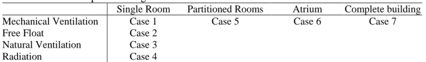
The first studied case comes from a study of Kuznik et al. (2007). It is a basic case without obstacle in the room (see Figure 1.a). The convection cell is created exclusively by the mechanical ventilation. The issue of jet description is approached.

3

Case 2: Free Float Case

This validation step is based on the experimental results obtain by Yuan et al. (1999). It describes the airflow in a typical office (see Figure 1.b). There is a displacement ventilation device but convection is mainly dominated by thermal loads (computers, lights, etc.). Indeed, the air velocity induced by the mechanical ventilation is very low (0.09 m/s).

a) b)

Figure 1. Illustrations of the cases. a) Mechanical Ventilation Case (Kuznik et al. 2007), b) Free Float Case (Yuan et al. 1999).

Case 3: Natural Ventilation Case

This case was first studied by Jiang and Chen (2003). There are two types of natural ventilation: buoyancy-driven and wind-driven ventilation (Jiang et al., 2004). Only the first case was retained because it is the most difficult to model, due to smaller pressure differences. Buoyancy-driven ventilation is also the most interesting case in temperate climate. Indeed, the “worst scenario” that could happen is a warm and windless day (Jiang and Chen, 2003). This case is a room inside another one which reproduces external conditions (see Figure 2.a).

Case 4: Radiation Case

Radiant panels are more and more used in buildings and the aim of this case is to make the operator able to describe correctly this type of installation. The experimental data comes from a study of the University of Liège led by Tang (1998). The test room is composed of two parts separated by an opening (see Figure 2.b). There is a heating wall in the smallest part. This subject is really important for building engineers and architects because radiative heating and cooling is more and more used in new buildings.

a) b)

Figure 2. Illustrations of the cases. a) Natural Ventilation Case (Jiang and Chen, 2003), b) Radiation Case (Tang 1998).

RESULTS

In this section, Fluent, widely used software in CFD, is submitted to our validation process. The first case is deeply analyzed in accordance with Chen and Srebric (2001) while only the graphical results of the three other cases will be presented.

4

Results obtained with Trnsys (dynamic multizone software) are also discussed. The reference papers being based on a CFD validation approach, all needed hypothesis were not available to run dynamic simulation. For example, the surface temperature of wall is sometimes given as a boundary condition for CFD models, while external climatic conditions used for multizonal approach are unknown. Some assumptions were made and are exposed in this section.

Case 1: Forced Convection Case

Geometrical description

This case is based on an experiment led by Kuznik et al. (2007). Geometrical data are available in the related paper so that operator can reproduce this validation case. As figure 1.a) indicates, this case is very basic: there is no obstacle inside the room and temperature are imposed on every wall.

Experiment description

Experimental velocity isovalue lines in the jet region will provide a qualitatively analysis while maximum velocity and maximum temperature decay will allow a quantitative comparison. These values are measured in the median plane (the jet plane, the most interesting one) and two consecutive measurements are separated by a distance of 0.1m. Every thermal measurement has a resolution of ±0.4°C and velocity measurement resolution is the worst of ±0.05m/s and ±3% of the measurement value for a temperature contained between 20°C and 26°C, adding 0.5%/°C outside this range.

Turbulence model

Shear-Stress Transport (SST) k-ω model (Menter, 1994) was chosen. Indeed, it was the one that gave the best results in the original article. It could be noted that two-equations k-ω models do not need special near-wall treatment, which is very appreciable when boundaries are mainly walls. Note that, for this reason, the three other cases use the same model.

Boundary conditions

There are three types of boundary in this case: an inlet, an outlet and walls. The first one was modelled simply by imposing a constant velocity profile. The second boundary type was modelled by a zero pressure outlet. The third one was modelled by imposing the wall surfaces temperature as described in Kuznik et al. (2007) and a no-slip condition.

Numerical methods

The Navier-Stokes equations were discretized by a finite volume method with a cell-based approach. For the velocity-pressure coupling, the SIMPLEC numerical algorithm was used. The derivatives were discretized with a QUICK scheme. To ensure the best convergence, the technique of Cook and Lomas (1997) was used (combination of under-relaxation and false time-stepping). Solution was considered as converged when no further change was noticed in the solution during one hundred iterations. Concerning the mesh, an unstructured approach was chosen because of curved surfaces. Results were obtained with a 600 000 tetrahedral cells mesh. Grid independence was checked with another mesh (two times bigger) and gave satisfactory results.

Results

Chen and Srebric (2001) suggested comparing firstly qualitatively the global aspect of the results with, for example, the velocity field. This is done at Figure 3 and shows a quite good agreement between the two approaches.

5

a) b)

Figure 3. Velocity isovalue lines. a) Experimental data, b) Numerical data

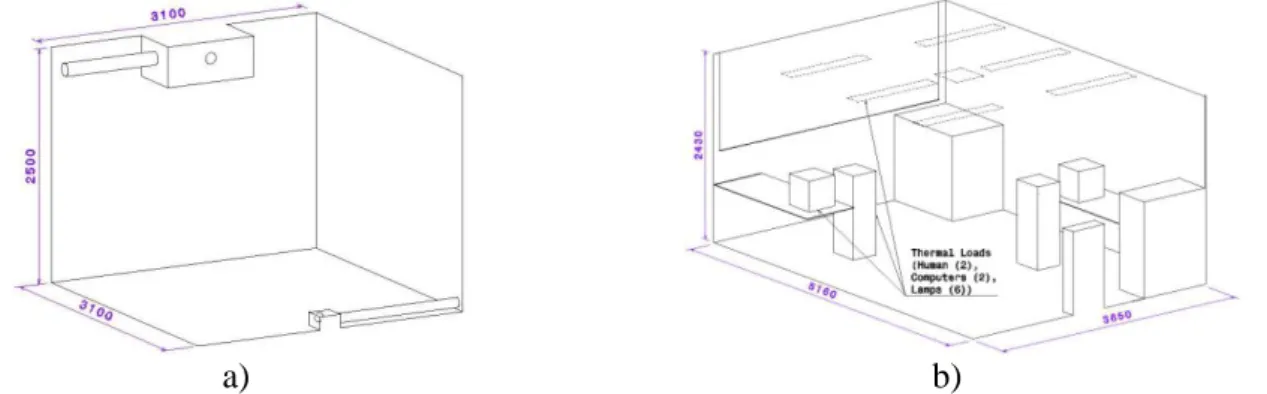
The second step imposes to compare quantitatively results. There is no criterion on the validity; everything depends on user’s expectations. The error should also be compared to the error made experimentally. In our case, results are provided at Figure 4. Agreement is very good, both for maximum velocity and maximum temperature decays. The mean error on velocity is inferior to 0.02m/s and the mean thermal error is 0.16°C. Given the range of these two variables, there is less than 5% of error which is very good. For the two variables, it should be noted that numerical results are always inside measurements incertitude which confirms Fluent’s ability to describe mechanical ventilation.

Figure 4. Mechanical Ventilation Case: Maximum temperature and velocity decay. Conclusions

Even if results are very good, some limitations should not be forgotten. For example, wall surface temperature is here a data but it is an unknown in most industrial cases. These values can be calculated by making the domain of simulation bigger or thanks to other software as multizone approaches. This will introduce more incertitude in the results. Another limitation lies in the fact that contaminant transport was not approached. This aspect is also very important in building physics simulations and needs to be validated prior to be useful. Concerning this case, the CFD code Fluent can give satisfactory results for mechanical ventilation if the operator has enough experience to use it adequately.

Case 2: Free Float Case

The results are drawn at Figure 5. This simulation was done with a k-ω turbulence model and a mesh of 422 544 tetrahedral cells. Numerical and experimental data are very close and two aspects of this simulation must be underlined: thermal stratification and very small velocities. The first aspect has very important implications. Multizone software cannot predict thermal stratification because it gives a mean result over the entire room. With CFD, it is possible to have a precise description of the thermal gradient and to predict temperatures inside the room. The second aspect is inherent to natural convection. This phenomenon is characterized by very small air velocities and body forces which are very critical for calculation stability (Cook and Lomas, 1997). Despite this, we can see that small velocities, on which there is important measure incertitude, are quite well described.

6 Figure 5. Results of the Free Float Case.

For multizonal simulations, every wall is modelled with a constant external temperature of 15°C. Results are in good agreement with experimental data. The mean air temperature is 24.82°C (see Fig. 6). Nevertheless, Yuan et al. (1999) gave an internal surface temperature range of 23.3 to 26°C. As shown in Fig.6, this range could be found with various external temperature hypotheses (from 11°C to 19°C). The impact on the ambient air temperature is around 1.5°C in this range. This proves one of the limitations of multizonal approaches.

Fig 6. Results of Multizonal Simulations for the Free Float Case

Case 3: Natural Ventilation Case

Results of this case are described in Figure 7. They were obtained with a 732 039 cells mesh and a k-ω turbulence model. Once again, even if air velocities are very small, results are very good. Concerning air temperatures, agreement is also reached. Figure 7 shows that temperature gradients are quite well captured even if thermal loads are big.

7

An interesting aspect of this case is the interaction between external and internal airflows. Air exchange rate was measured and the result varied between 6.75 and 7.92 Air Changes per Hour (ACH) in the test-room. CFD gives a slightly overestimating value of 7.95. This result is satisfactory, but it could be improved by using a LES method for turbulence modelling. With Trnflow simulations, the result is 8.47 ACH. This result proves the limitations of multizonal simulations but the very small computing time needed is valuable in a preliminary design. But for other cases described in that paper by Jiang et al. (2004) (the door cases), multizonal simulations do not give satisfactory results. Indeed, 17.05 ACH are simulated with Trnflow while between 9.18 and 12.6 ACH are measured. According to Wang and Chen (2008), this could be explained by thermal stratification which is not correctly considered in a multizonal approach. The dimensionless gradient of temperature τ which should not exceed 0.03 according to Wang and Chen (2008) is 0.117 in both “window” and “door” cases. From these results, it appears that the dimensionless limitations do not exactly indicate the limitations of multizonal approaches and should be considered simultaneously with the size of the opening.

Case 4: Radiation Case

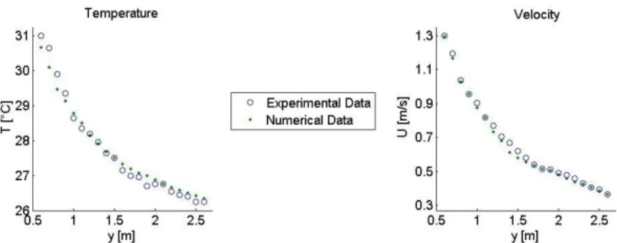
Results for the air temperature for the radiation case are shown in Figure 8. A mesh of 371 824 tetrahedral cells and a k-ω turbulence model were used. As for the other cases, it can be seen that thermal gradients obtained numerically are in good agreement with experimental ones. The air temperature mean error is inferior to 0.2°C. It should be noted that air velocities in the central opening between the two rooms are also well simulated (mean error of 0.01m/s).

Figure 8. Results of the Radiation Case.

DISCUSSIONS

Results for each case prove clearly that CFD represents a new reliable solution. Thanks to numerical simulations, it is now possible to predict correctly airflows in buildings. The good agreement between experimental and numerical data validates the use of Fluent for the four cases. With this methodology, architects and building engineers will be able to compare and calibrate their own results with experimental and numerical results described above. Multizonal simulations also show good agreement. Despite this, it is suspected that further exploration of the test cases will identify specific limitations for both approaches.

The interest of CFD is not to replace older tools (as multizone simulations) but to help to get a better prediction in the design stage for some important parameters like temperature

8

stratification or air velocity in rooms. Indeed, CFD, unlike multizone software, is still unable to predict correctly thermal boundary conditions (wall temperature or heat transfer).

CONCLUSIONS

This paper was made to fill in a void. It aims to create a tool that will help architects and building engineers to become confident in CFD simulations. We proposed a validation process dealing with four physical phenomena occurring in building physics: free float, mechanical ventilation, natural ventilation and radiation. This validation and learning process studies building physics phenomena in a room.

Compared with thermal multizonal simulation tools, CFD simulations provide gradients of temperature, airflows and air velocities in a room. Consequently, occupant’s comfort is predictable. The use of CFD will thus permit to improve projects realization and to prevent classical errors in buildings (lack of ventilation, overheating, etc.). Eventually, one should not forget that numerical simulations can greatly improve building energy performance, one of the main challenges of this century, but also IAQ and occupant’s comfort.

ACKNOWLEDGEMENT

This research is a part of the SIMBA project. It is supported by the European Regional Development Fund (ERDF) and the Walloon Region. We gratefully thank the reviewers for their comments which helped to improve the quality of this paper.

REFERENCES

ANSYS Inc. 2009. ANSYS Fluent 12.0 Documentation (Version 12.0.16).

Cook M.J. and Lomas K.J. 1997. Guidance on the use of computational fluid dynamics for modelling buoyancy driven flows. In: Proceedings of the IBPSA Building Simulation ’97, Prague, Vol. 3, pp. 57-72.

Chen Q. and Jiang Z. 1992. Significant questions in predicting room air motion. ASHRAE Transactions, 98, 929-939.

Chen Q. and Srebric J. 2001. How to verify, validate, and report indoor environment modeling CFD analysis. ASHRAE, ASHRAE RP-1133.

Jiang Y. and Chen Q. 2003. Buoyancy-driven single-sided natural ventilation in buildings with large openings. International Journal of Heat and Mass Transfer, 46, 973-988. Jiang Y., Alloca C. and Chen Q. 2004. Validation of CFD simulations for natural ventilation.

International Journal of Ventilation, 2(4), 359-370.

Kuznik F., Rusaouën G. and Brau J. 2007. Experimental and numerical study of a full scale ventilated enclosure: Comparison of four two equations closure turbulence models. Building and Environment, 42, 1043-1053.

Menter F.R. 1994. Two-equation eddy-viscosity turbulence models for engineering applications. AIAA Journal, 32(8), 1598-1605.

Tang D. and Robberechts B. 1989. Interzone convective heat transfer and air flow patterns. Report of Laboratory of Thermodynamics, University of Liege (Belgium).

Tang D. 1998. CFD modelling and experimental validation of air flow between spaces. In: Proceedings of the 6th International Conference on Air Distribution in Rooms – Roomvent 98, Stockholm, Vol. 2, pp. 547-554.

Wang L. and Chen Q. 2008. Evaluation of some assumptions used in multizone airflow network models. Building and Environment, 43(10), 1671-1677.

Yuan X., Chen Q., Glicksman L.R., Hu Y. and Yang X. 1999. Measurements and computations of room airflow with displacement ventilation. ASHRAE Transactions, 105(1), 340-352.