2018 — Numerical enhancement of a mesoscale model for large-eddy simulation of the wind over steep terrain

WIND OVER STEEP TERRAIN

by

Alex Geovanny FLORES MARADIAGA

MANUSCRIPT-BASED THESIS PRESENTED TO ÉCOLE DE

TECHNOLOGIE SUPÉRIEURE IN PARTIAL FULFILLMENT OF THE

REQUIREMENTS FOR THE DEGREE OF DOCTOR OF PHILOSOPHY

PH.D.

MONTRÉAL, QC, NOVEMBER 05, 2018

ÉCOLE DE TECHNOLOGIE SUPÉRIEURE

UNIVERSITÉ DU QUÉBEC

This Creative Commons licence allows readers to download this work and share it with others as long as the author is credited. The content of this work can’t be modified in any way or used commercially.

BY THE FOLLOWING BOARD OF EXAMINERS

Mr. Robert Benoit, Ph.D., Thesis Supervisor

Department of Mechanical Engineering at École de technologie supérieure Mr. Christian Masson, Ph.D., Thesis Co-Supervisor

Department of Mechanical Engineering at École de technologie supérieure Mr. Francois Brissette, Ph.D., President of the Board of Examiners

Department of Civil Engineering at École de technologie supérieure Mr. Louis Dufresne, Ph.D., Member of the Jury

Department of Mechanical Engineering at École de technologie supérieure Mr. Peter Taylor, Ph.D., External Evaluator

Department of Earth and Space Science and Engineering at York University

THIS THESIS WAS PRENSENTED AND DEFENDED

IN THE PRESENCE OF A BOARD OF EXAMINERS AND PUBLIC AUGUST 24, 2018

FOREWORD

This thesis follows a sequential format of three journal articles, each presenting original work on different but interrelated topics. This work was conducted by myself as the principal author in conjunction with various collaborators who have been duly acknowledged. The referred journal articles are included in the thesis as follows:

Chapter 2 is based on the article entitled “Numerical Stability and Noise Control with a New Semi-Implicit Scheme for Mesoscale Modelling over Steep Terrain”, submitted to the journal Boundary-Layer Meteorology. This work was orally presented at the CanWEA 28th _Annual Conference and Exhibition (Toronto, ON, October 14-17, 2012) and a poster was presented at AWEA 2013 WINDPOWER Conference and Exhibition (Chicago, IL, May 5-7, 2013). Chapter 3 refers to the article entitled “Enhanced Mesoscale Modelling of the Stratified Surface Layer over Steep Terrain for Wind Resource Assessment”, submitted to the journal Boundary-Layer Meteorology. An oral presentation of this work was made at the CanWEA 30th _Annual Conference and Exhibition (Montréal, QC, October 27-30, 2014), and a poster was also presented at the 16th _{Chilean Conference of Mechanical Engineering (Valparaiso, Chile,} November 18-20, 2015).

Chapter 4 presents the article entitled “Wind Modelling over Steep Terrain with Large Eddy Simulation Embedded in a Mesoscale Atmospheric Model”, submitted to the journal Boundary-Layer Meteorology. A poster presentation on the progress of this work was made at the 6th _{TORQUE International Conference “The Science of Making Torque from Wind”} (Munich, Germany, October 5-7, 2016), and the final results were presented at the AWEA 2017 WINDPOWER Conference and Exhibition (Anaheim, CA, May 22-25, 2017).

ACKNOWLEDGMENT

I want to sincerely and gratefully thank Dr. Robert Benoit and Dr. Christian Masson, co-directors of this doctorate, for your mentorship, support and patience throughout this research project. With your constant motivation and guidance I was able to accomplish successfully this endeavour, and from you I have learned significantly how to collaborate with other researchers in scientific projects. Moreover, I wish to thank Dr. Claude Girard and Dr. Nicolas Gasset for your guidance, encouragement and fruitful discussions throughout my doctorate. Your scientific contributions are the cornerstone of this project, and I will always be grateful for all the ideas and time you dedicated to help and teach me.

I greatly thank as well Dr. Louis Dufresne, Dr. François Brissette and Dr. Peter Taylor, for taking time to read and evaluate this thesis. To Fayçal Lamraoui, Philippe Pham, Mary Bautista, Hugo Olivares, Yann-Aël Muller, Hajer Ben Younes, Jörn Nathan, Pascal Doran and many more of my colleagues at the Research Laboratory on the Nordic Environment Aerodynamics of Wind Turbines (NEAT), thank you very much for your help and friendship. In addition, I am truly thankful to my wonderful friends Cristóbal Ochoa, Marthy García, Alejandra Frontana, Virgilio Quintana, Gabriel Astudillo and all the troupe of the Jeunesse X-Cathedra for the greatest memories I keep of my life in Montréal.

I also want to thank the Wind Energy Strategic Network (WESNet) of the Natural Sciences and Engineering Research Council of Canada (NSERC), the École de Technologie Supérieure and the Federico Santa María Technical University for their scholarships, grants and the facilities provided. I believe it is a great honor to belong and work in these remarkable institutions, where one can learn greatly of advanced engineering and innovation. Likewise, I acknowledge the research group Recherche en Prévision Numérique (RPN) from Environment Canada for its technical support, and for sharing the novel version of the Mesoscale Compressible Community (MC2) model source code.

I definitely want to thank my mother Afrodita and dear family for all your love and immense support since my birth and at every step I have taken during this doctorate. Finally, very special thanks to my beloved wife Marina; you have always been my greatest inspiration and supporter in this endeavour.

This work is dedicated to my beloved children, the most amazing blessings of all. To them I wish to underline that, just when you think you know love something so beautiful as family comes along to remind you just how big it really is. The time I spend with you is gold, and your health and well-being are my wealth. Be the best people you can be and always follow your heart and Holy Spirit.

AMÉLIORATION NUMÉRIQUE D'UN MODÈLE MÉSOÉCHELLE POUR LA SIMULATION AUX GRANDES ECHELLES DU VENT SUR TERRAIN ESCARPÉ

Alex Geovanny FLORES MARADIAGA

RÉSUMÉ

La modélisation à mésoéchelle de la couche limite atmosphérique a progressé de manière significative au cours des dernières décades, bien qu'il y ait encore des aspects numériques qui doivent être améliorés pour obtenir des simulations de vent précises sur une topographie escarpé. Ceci est devenu une nécessité puisque de nombreuses applications, telles que l'évaluation des ressources éoliennes, exigent maintenant des résultats de haute fidélité pour l'analyse de la viabilité et la prise de décision. Avec l'arrivée de l'informatique de haute performance et de logiciels plus sophistiqués, l'industrie de l'énergie éolienne s'intéresse de plus en plus aux modèles multi-échelles basés sur des configurations combinées capables de produire des résultats à plus haute résolution. La taille des parcs éoliens modernes nécessite maintenant une analyse multi-échelle qui permet l'évaluation des processus méso- et micro-échelle déclenchés sur topographie complexe. Pour cette raison, les modèles à mésomicro-échelle avec des capacités de large-eddy simulation sont bien adaptés pour devenir la prochaine grande famille de kits de simulation pour l'ingénierie éolienne.

Le modèle MC2 (Mesoscale Compressible Community), sujet de ce travail, est un bon exemple puisqu'il est utilisé comme noyau du Wind Energy Simulation Toolkit (WEST), présentée par le groupe RPN d'Environnement Canada. MC2 se comporte bien pour les simulations du vent sur terrain plat et sur des pentes douces et modérées, ce qui a amené la communauté de l'énergie éolienne à être confiante pour l'utiliser pour générer l'Atlas éolien du Canada. Cependant, comme avec d'autres modèles similaires, plusieurs problèmes numériques tels que la surestimation du vent et des circulation distorsionnées ont été identifiés ces dernières années à partir de simulations d'écoulement orographique en présence de fortes pentes. Par conséquent, l'évaluation des ressources éoliennes au-dessus d'une topographie à fort impact, comme les Montagnes Rocheuses ou l'escarpement du Niagara, ne peut pas être entièrement fiable et nécessite une réévaluation avec une modélisation multi-échelle améliorée.

En appliquant une analyse spectral, nous avons reconnu l'instabilité numérique et mesuré avec précision le bruit parasite inhérent au schéma semi-implicite (SI) classique à trois niveaux de temps de MC2. Avec la redéfinition appropriée des variables thermodynamiques pronostiques, la discrétisation temporelle SI, couplée au schéma semi-lagrangien (SL), est maintenant structurée de façon à permettre à MC2 de résoudre les équations d'Euler (EE) non-hydrostatiques compressibles dans une mode plus stable et précise. MC2 est maintenant capable d'effectuer des simulations du vent sur des pentes abruptes en l'absence de décentrage temporel, de filtre de fréquence et d'autres mécanismes d'amortissement numérique. En outre, la classification de la méthode Statistical Dynamical Downscaling (SDD) est améliorée en incluant la fréquence de Brunt-Väisälä qui tient compte de l'effet de stratification thermique atmosphérique sur le débit du vent par rapport à la topographie. La présente étude fournit une vraie validation orographique de ces améliorations numériques dans MC2, en évaluant leur

contribution individuelle et combinée pour une meilleure initialisation et un calcul du vent de surface en présence de terrain à fort impact.

Enfin, l'adaptation du tenseur métrique de la méthode de simulation aux grandes échelles (LES) implémenté dans MC2, nécessaire à la modélisation du vent sur les terrains montagneux, a été réalisé en préservant la stabilité et la précision numériques améliorées. Les résultats des tests indiquent que le modèle MC2-LES amélioré reproduit efficacement les modèles d'écoulement prévus, la séparation et la recirculation sur terrain escarpé et donne des résultats précis comparables à ceux rapportés par les données expérimentales ou par d'autres chercheurs utilisant des modèles numériques avec des systèmes de fermeture de turbulence plus sophistiqués.

Mots-clés: couche limite atmosphérique, évaluation des ressources éoliennes, modélisation

mésoéchelle, simulation aux grandes échelles, terrain complexe, bruit numérique, stabilité numérique, schéma semi-implicite, écoulement du vent à stratification neutre

NUMERICAL ENHANCEMENT OF A MESOSCALE MODEL FOR LARGE-EDDY SIMULATION OF THE WIND OVER STEEP TERRAIN

Alex Geovanny FLORES MARADIAGA

ABSTRACT

Mesoscale modelling of the atmospheric boundary layer has advanced significantly over the past decades, although there are still different numerical aspects that must be enhanced to achieve accurate wind simulations over steep topography. This has become a necessity since many applications, such as wind resource assessment, now require high fidelity results for viability analysis and decision-making. With the advent of high performance computing and more sophisticated software, the wind energy industry is increasingly interested in multiscale models based on combined configurations capable of yielding higher resolution results. The size of the modern wind farms now requires a multiscale analysis that allows the evaluation of the joint meso- and microscale processes triggered over complex topography. For this reason, mesoscale models with imbedded large-eddy simulation capabilities are well suited to become the next mainstream family of simulation toolkits for wind engineering.

The Mesoscale Compressible Community (MC2) model, subject of this work, is a good example since it is employed as the kernel of the Wind Energy Simulation Toolkit (WEST), introduced by the Recherche en Prévision Numérique (RPN) group of Environment Canada. MC2 performs well for wind simulations over flat, gentle and moderate terrain slopes, which led the wind energy community to be confident enough on employing it to generate the Canadian Wind Atlas. However, as with other similar models, several numerical issues such as wind overestimation and distorted circulation patterns have been identified in recent years from orographic flow simulations in presence of steep slopes. Hence, wind resource assessment over high impact topography, such as the Rocky Mountains or the Niagara Escarpment, cannot be entirely reliable and needs a revaluation with enhanced multiscale modelling.

By applying an eigenmode analysis, we have recognized the numerical instability and precisely measured the spurious noise problem, inherent of MC2’s classical three time-level semi-implicit (SI) scheme. With the appropriate redefinition of the prognostic thermodynamic variables, the SI time discretization, coupled with the semi-Lagrangian (SL) scheme, is now consistently structured in a way that it enables MC2 to solve the compressible non-hydrostatic Euler equations (EE) in a more stable and accurate fashion. MC2 is now able to perform wind simulations over steep slopes in the absence of time decentering, frequency filtering and other numerical damping mechanisms. Additionally, the climate-state classification of the statistical-dynamical downscaling (SDD) method is upgraded by including the Brunt-Väisälä frequency that accounts for the atmospheric thermal stratification effect on wind flow over topography. The present study provides a real orographic flow validation of these numerical enhancements in MC2, assessing their individual and combined contribution for an improved initialization and calculation of the surface wind in presence of high-impact terrain.

Lastly, the metric tensor adaptation of MC2’s imbedded large-eddy simulation (LES) method, necessary for wind modelling over mountainous terrain, has been achieved preserving the enhanced numerical stability and accuracy. Test results indicate that the enhanced MC2-LES model reproduces efficiently the expected flow patterns, separation and recirculation zone over steep terrain, and yields accurate results comparable to those reported from experimental data or by other researchers who use numerical models with similar or more sophisticated turbulence closure schemes.

Keywords: atmospheric boundary layer, wind resource assessment, mesoscale modelling,

large-eddy simulation, complex terrain, numerical noise, numerical stability, semi-implicit scheme, neutrally stratified wind flow

TABLE OF CONTENTS

Page

INTRODUCTION ... 1

CHAPTER 1 ATMOSPHERIC BOUNDARY LAYER FUNDAMENTALS AND MODELLING – CONCEPTUAL FRAMEWORK AND LITERATURE REVIEW ... 11

1.1 Dynamics of the Atmospheric Boundary Layer (ABL) ... 12

1.1.1 Atmospheric Thermal Stratification and the ABL Structure ... 17

1.1.2 Rotational and Topographic Effects on Stratified ABL Flow ... 21

1.1.3 Turbulence and Diffusion in Stratified ABL Flow ... 26

1.2 Numerical Modelling of Stratified ABL Flow over Complex Terrain ... 32

1.2.1 Coupling Large-Eddy Simulation (LES) with Mesoscale Modelling .... 34

1.2.2 The Mesoscale Compressible Community (MC2) Model ... 37

1.2.3 Numerical Stability of the SISL Leapfrog Method ... 42

1.2.4 Model Equations Filtering and Turbulence Parameterization ... 46

1.2.5 Boundary Conditions and Computational Grid ... 49

CHAPTER 2 NUMERICAL STABILITY AND NOISE CONTROL OF A NEW SEMI-IMPLICIT SCHEME FOR MESOSCALE MODELLING OVER STEEP TERRAIN ... 57

2.1 Background and Context... 58

2.2 Basic Semi-discrete Model Equations ... 62

2.3 Stability Analysis of the Original SI (O-SI) Scheme ... 65

2.4 The New Semi-implicit (N-SI) Scheme ... 71

2.5 Validation and Discussion ... 75

2.5.1 Atmosphere-at-rest Simulations with Different Terrain Slopes ... 76

2.5.2 Atmosphere-at-rest Simulations with Different Parametric Combinations ... 83

2.5.3 Atmosphere-at-rest Multi-layer Simulations over Steep Parallel Ridges87 2.6 Summary ... 92

CHAPTER 3 ENHANCED MESOSCALE MODELLING OF THE STRATIFIED SURFACE LAYER OVER STEEP TERRAIN FOR WIND RESOURCE ASSESSMENT ... 95

3.1 Background and Context... 96

3.2 Model Description and Main Issues ... 100

3.3 Model Enhancement ... 104

3.3.1 The New Wind Climate-state Classification for the SDD Method ... 104

3.3.2 The New Semi-Implicit (N-SI) Scheme for Numerical Noise Reduction ... 107

3.4 Validation and Discussion ... 108

3.4.2 Numerical Simulation of Strongly Stratified Wind over the Whitehorse

Valley ... 116

3.5 Summary ... 123

CHAPTER 4 WIND MODELLING OVER STEEP TERRAIN WITH LARGE EDDY SIMULATION EMBEDDED IN A MESOSCALE ATMOSPHERIC MODEL ... 125

4.1 Background and Context... 126

4.2 Model Equations and Numerical Enhancements ... 130

4.3 Validation and Discussion ... 135

4.3.1 Neutral ABL Simulations over Flat Terrain for Model Calibration .... 138

4.3.2 Neutral ABL Simulations over an Isolated Gaussian Ridge ... 146

4.3.3 Neutral ABL Simulations over the RUSHIL H3 Ridge ... 151

4.4 Summary ... 158

CONCLUSIONS ... 161

APPENDIX I Surface Stress Calculation with the Oblique Coordinate System for Complex Terrain ... 165

APPENDIX II Extended Stability Analysis of the 3-TL O-SI Scheme Applied to the EE System in Height Based σ-coordinate ... 167

APPENDIX III Extended Stability Analysis of the 3-TL N-SI Scheme Applied to the EE System in Height Based σ-coordinate ... 171

APPENDIX IV Metric Terms for MC2-LES Turbulent Diffusion Formulae ... 175

LIST OF TABLES

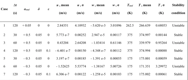
Page Table 2.1 Statistical results after 24 h for isothermal atmosphere-at-rest

experiments with the O-SI scheme over flat terrain, varying the time-step (_{Δ ), surface temperature ratio (}t _{α ), Robert-surf}

Asselin time-filter (δ ) and time decentering coefficient (ε ) ... 69 Table 2.2 Different parametric combinations of terrain slope (ϑ),

time-step (_{Δ ), grid resolution (}t _{Δ Δ}x, z), surface temperature ratio (_{α ), and Brunt-Väisälä frequency ( N ) for atmosphere-at-rest surf}

experiments with the N-SI scheme ... 83 Table 3.1 Description of the wind stations distributed in the Whitehorse

valley ... 112 Table 3.2 Ensemble statistics of the mesoscale simulations of surface wind

LIST OF FIGURES

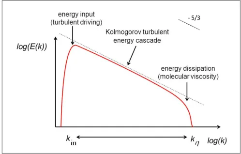
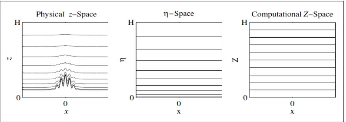
Page Figure 1.1 Energy spectrum of a well-developed turbulent flow ... 27 Figure 1.2 Height of the computational levels in physical z-coordinates

(left), Gal-Chen η-coordinates (middle) and computational

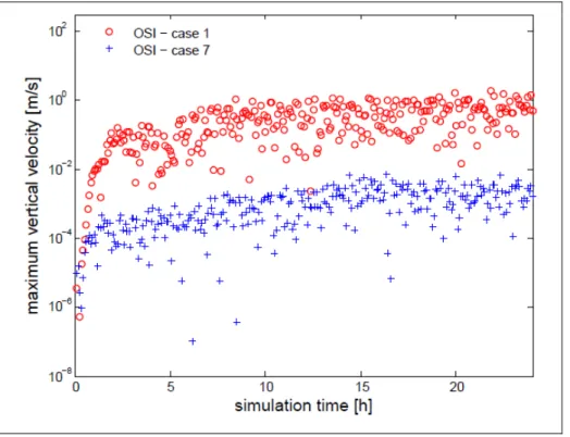
Z-coordinates (right). Leuenberger et al. (2010) ... 52 Figure 2.1 Maximum vertical velocity w_max 24 h evolution for the

resting-atmosphere cases 1 and 7 of Table 2.1, done with the O-SI

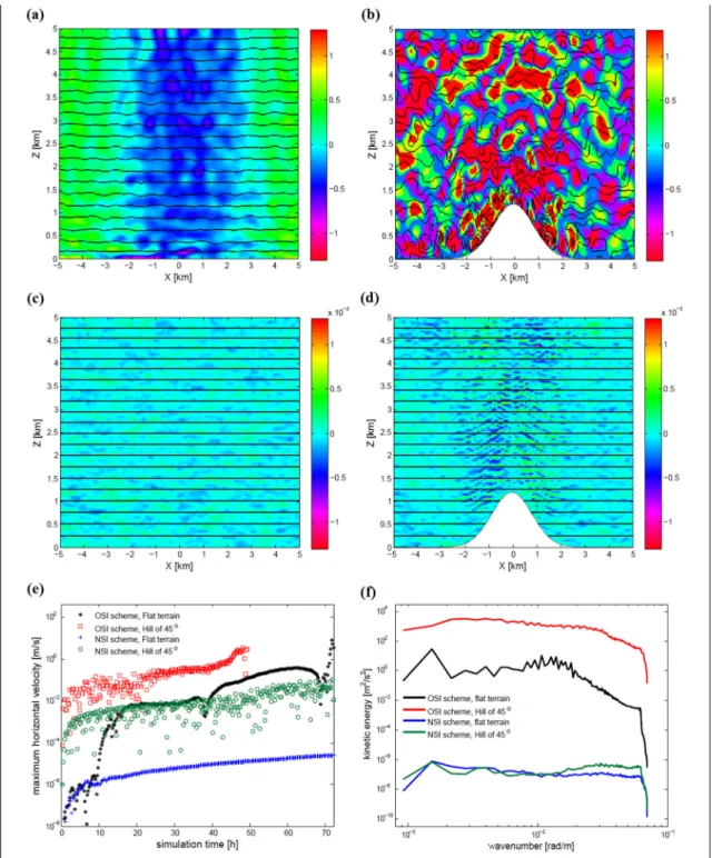
scheme ... 70 Figure 2.2 Horizontal velocity field cross-sections at 42 h, for an isothermal

atmosphere initially at rest over flat terrain and a steep mountain, employing the O-SI scheme in panels (a) and (b) and the N-SI scheme in panels (c) and (d). Solid lines denote potential temperature isentropes (interval of 2.5 K) and color shading the horizontal velocity (ms-1_{). Panels (e) and (f) respectively} illustrate the evolution of the absolute maximum horizontal

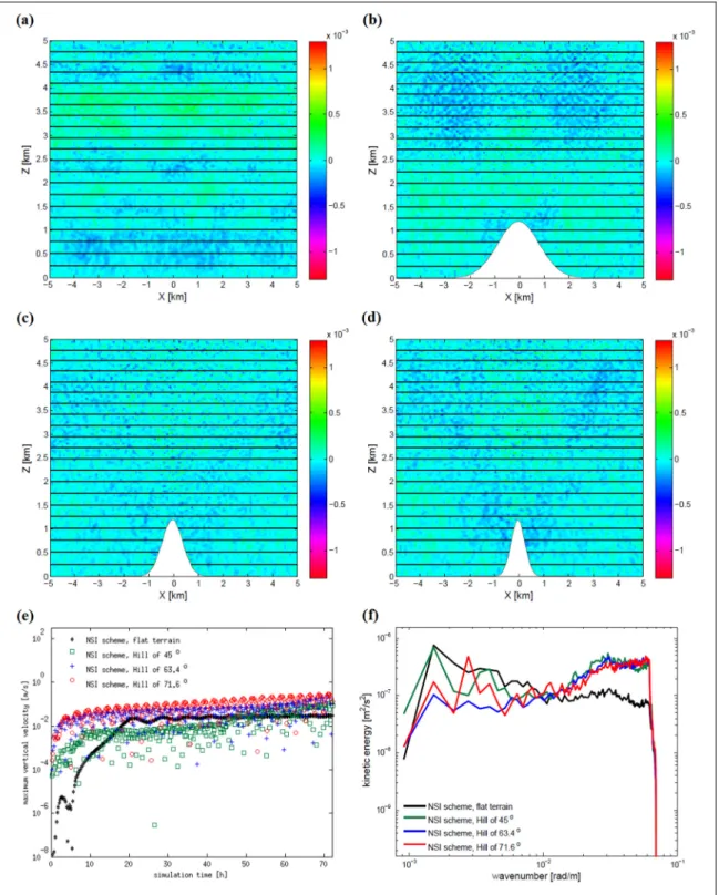
velocity u_max and the 2D kinetic energy spectra of noise ... 78 Figure 2.3 As in Figure 2.2, but comparing the vertical velocity

cross-sections, w_maxevolution and kinetic energy spectra of an isothermal atmosphere initially at rest using the N-SI scheme over (a) flat terrain and a Gaussian hill with maximum slope of

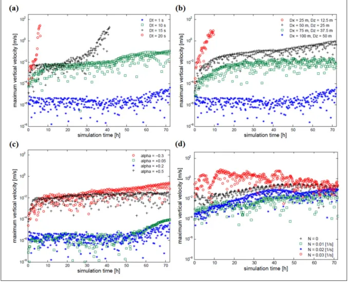
(b) 45 °, (c) 63.4 ° and (d) 71.6 °, respectively ... 80 Figure 2.4 Evolution of the maximum vertical velocity w_max with the N-SI

scheme when varying (a) time-step, (b) grid resolution, (c)

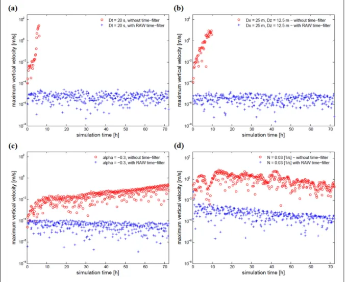
surface temperature and (d) stratification ... 85 Figure 2.5 As in Figure 2.4, but using the combined N-SI scheme and RAW

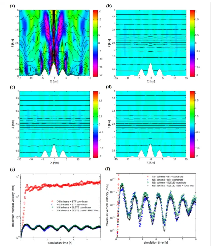
time-filter for the previous unstable resting-atmosphere tests ... 87 Figure 2.6 Vertical velocity cross-sections at t= 6 h for a non-isothermal

resting-atmosphere over the classic Schär mountain tested with the combined (a) O-SI scheme + BTF coordinate, (b) N-SI scheme + BTF coordinate, (c) N-SI scheme + SLEVE coordinate and (d) N-SI scheme + SLEVE coordinate + RAW time-filter. Panel (e) shows the time evolution of w_max, and panel (f)

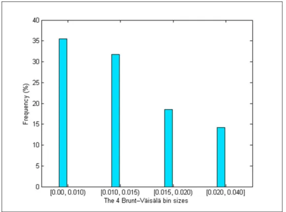
Figure 3.1 Frequency of (a) neutral [0 - 0.01[ s-1_{, (b) slightly stable [0.01 -} 0.015[ s-1_{, (c) stable [0.015 - 0.02[ s}-1 _{and (d) strongly stable}

[0.02 - 0.04] s-1 _{thermal stratification in the Whitehorse area ... 106} Figure 3.2 Three-dimensional illustrations of the (a) Whitehorse area at 5

km resolution and (b) Whitehorse valley at 1 km resolution ... 110 Figure 3.3 Wind stations distributed within the Whitehorse valley, at

Yukon Territory of Western Canada, measuring meteorological

conditions at 30 m above ground level ... 111 Figure 3.4 Vertical velocity cross-sections of four climate-states with the

same mean wind speed of 7 ms-1_{, wind direction of 225 degrees} and positive shear, classified with different Brunt-Väisälä frequencies of (a) 0.0091 s-1_{, (b) 0.0137 s}-1_{, (c) 0.0174 s}-1 _{and (d)}

0.022 s-1_{, respectively ... 114} Figure 3.5 Time evolution of the numerical noise for (a) stream-wise and

(b) span-wise surface wind speeds (ms-1_{) at the Whitehorse # 1}

wind station ... 115 Figure 3.6 Wind speed (ms-1_{) distribution (left panels) and comparison of}

modeled versus observed wind speeds (right panels) over the Whitehorse area, obtained with the OC+OSI combination implemented in (a)-(b) MC2 v4.9.6 and (c)-(d) MC2 v4.9.8,

respectively ... 118 Figure 3.7 Wind speed (ms-1_{) distribution (left panels) and comparison of}

modeled versus observed wind speeds (right panels) over the Whitehorse area, obtained with the (a)-(b) NC+OSI, (c)-(d) OC+NSI and (e)-(f) NC+NSI combinations implemented in

MC2 v.4.9.9 ... 120 Figure 3.8 Mean wind flow patterns at 30 m AGL in the Whitehorse valley,

obtained with the (a) OC+OSI and (b) NC+NSI combinations

implemented in MC2 v.4.9.9 ... 122 Figure 4.1 Spatial distribution of model variables and constants in the

Arakawa C-type grid, for which _φ= f S K K, , _M, _T and , , ,

w T b TKE

ψ = ... 137 Figure 4.2 Evolution of the non-stationarity parameters for the (a)

stream-wise and (b) span-stream-wise velocity components of the EL over flat

Figure 4.3 Ensemble averaged (a) u and v velocity components, (b) wind non-dimensional gradient, (c) resolved and SGS τ₁₃ stresses, (d) resolved velocity variances, (e) resolved TKE and (f) energy

spectra in the flow’s interior and surface layer over flat terrain ... 141 Figure 4.4 Evolution of the non-stationarity parameters for the (a)

stream-wise and (b) span-stream-wise velocity components of the EL over flat

terrain, as function of the time cycles ... 143 Figure 4.5 Ensemble averaged (a) streamwise and spanwise velocity

components, (b) resolved and SGS normalized τ₁₃ stresses, (c)

resolved velocity variances and (d) surface layer energy spectra ... 146 Figure 4.6 (a) Schematic view of the Gaussian ridge geometry and (b)

locations of the [A] hill crest, [B] downslope lee-side and [C]

base valley over the Gaussian ridge ... 147 Figure 4.7 Time and span-wise averaged (a) wind speed and (b) resolved

and SGS parts of the τ₁₃ stress within the surface layer at the [A] hill crest, [B] downslope lee-side and [C] base valley along the

Gaussian ridge ... 148 Figure 4.8 Time averaged wind fields (ms-1_{) at 10 m a.g.l. over the}

symmetric Gaussian ridge with both SI schemes combined with

the Smagorinsky turbulence closure ... 150 Figure 4.9 Schematic view of the RUSHIL H3 ridge with the locations of

the [A] upslope, [B] hill crest, [C] downslope lee-side and [D]

base valley control stations, as in Allen and Brown (2002) ... 152 Figure 4.10 Time and span-wise averaged wind speed at the (a) upslope, (b)

hill crest, (c) downslope and (d) base points of the H3 ridge. As

in AB02, the ordinate is compared to the hill’s full-width 2a ... 153 Figure 4.11 Time-averaged (a) vertical flow field contours and vector

depiction at the transverse centerline, with ∗ representing the observed H3 separation streamline, and (b) horizontal winds

ref

U

u~ at _z≈7×10−3_{m a.g.l., the first internal momentum level ... 155}

Figure 4.12 Time and spanwise averaged normalized τ₁₃ stress at the (a) upslope, (b) hill crest, (c) downslope and (d) base positions of

Figure 4.13 Time and spanwise averaged normalized SGS τ₁₃ stress at the (a) upslope side, (b) hill crest, (c) downslope and (d) base

LIST OF ABREVIATIONS

3TL Three time levels agl Above ground level

ABL Atmospheric Boundary Layer AR-WRF Advanced Research WRF Model ARPS Advanced Regional Prediction System

B03 Bénard (2003)

B04 Bénard et al. (2004) B05 Bénard et al. (2005)

BTF Basic Terrain Following coordinate CFD Computational Fluid Dynamics

CFL Courant–Friedrichs–Lewy number

COAMPS Coupled Ocean/Atmosphere Mesoscale Prediction System CWE Computational Wind Engineering

DES, DNS Detached Eddy Simulation; Direct Numerical Simulation DRM Dynamic Reconstruction Model

EC Environment Canada

EE Euler Equations

EPA Environment Protection Agency FEM Finite Element Method

FVM Finite Volume Method

GEM Global Environment Multiscale unified model GMRES Generalized Minimal Residual iterative solver

GW Gigawatts HAZ High Accuracy Zone

HPC High Performance Computing IOP Intense Observation Period LAM Limited Area Model

LES Large Eddy Simulation LIDAR Light Detection and Ranging

MAP Mesoscale Alpine Programme MC2 Mesoscale Compressible Community Model MC2-LES MC2 model with LES capability

ML Mixed Layer

MM5 Mesoscale Model version 5 MO Monin-Obukhov MW Megawatts

NCAR National Center for Atmospheric Research NH Non-Hydrostatic

NS Navier-Stokes

N-SI New Semi-Implicit scheme NWP Numerical Weather Prediction O-SI Original Semi-Implicit scheme RAMS Regional Atmospheric Modeling System RANS Reynolds Averaged Navier-Stokes RA Robert-Asselin filter

RAW Robert-Asselin-Williams filter

RE Renewable Energy

RMSE Root Mean Square Error

RPN Recherche en Prévision Numérique RSM Reynolds Stress Model

SBL Stable Boundary Layer

SDD Statistical Dynamical Downscaling

SFS Sub-Filtered Scale

SGS Sub-Grid Scale

SHB78 Simmons, Hoskins and Burridge (1978) SI Semi-Implicit

SISL Semi-Implicit Semi-Lagrangian SL Semi-Lagrangian

SLEVE Smooth Level Vertical coordinate SODAR Sonic Detection and Ranging SSL Shear Surface Layer

TKE Turbulent Kinetic Energy TWh Terawatt-hour UKMO United Kingdom Met Office

URANS Unsteady Reynolds Averaged Navier-Stokes

US United States

WAsP Wind Atlas Analysis and Application Program WRF Weather Research and Forecast

LIST OF SYMBOLS Constants

p

c _{Heat capacity at constant pressure (1005 J kg-1 K-1)}

R Ideal gas constant (287.06 J kg-1 K-1)

s

p Surface reference pressure (1013.25 mbar)

g Gravitational acceleration of a fluid particle (9.81 ms-2)

υ Dry air kinematic viscosity (1.568×10-5 m2s-1)

κ Von Kármán non-dimensional constant (0.41)

π Pi number (3.14159)

π Euler number (2.71828)

c

Ri Critical Richardson constant (0.25)

Mathematical Operators and Notation

, ,

i j k Unit directional vectors in Cartesian coordinates

i

e Unit directional vector using Einstein’s notation

( ) ( )

( ) ( )

( )

∂ Local rate of change of a fluid’s quantity

( )

∇ Gradient of a fluid’s quantity

( )

H

∇ Horizontal 2D gradient of a fluid’s quantity

( )

∇ ⋅ Divergence of a fluid’s quantity

( )

2

∇ Lapacian, or gradient of the divergence, of a fluid’s quantity

( )

ρ

∇⋅ v Advection of a fluid’s quantity

( )

d dt Total or material derivative of a fluid’s quantity

( )

Spatial average

Ensemble average

j iu

u′ ′ Sub-filter velocity covariance or momentum flux

i iu

u′ ′ Sub-filter velocity variance

j

u′

′

ij

δ Kronecker delta rank-2 tensor

ijk

ε Levi-Civita spatial orientation rank-3 tensor

Greek Symbols

ρ _{Dry air density}

ρ′ _{Dry air density perturbation}

θ Dry air potential temperature

θ′ Dry air potential temperature perturbation

π Exner equation for pressure and temperature relationship

ψ _{Model variables}

ψ Model variable time average ψ′ _{Model variable perturbation}

t

ψ _{Model variable treated implicitly}

φ Model solution

λ Solution’s asymptotic growth rate

δ Time filtering coefficient

RAW

α _{Robert-Asselin-Williams (RAW) filter strength}

ξ _{Time decentering coefficient}

γ∗ _{Reference ABL height}

γ _{Ekman parametric constant}

Ω Planet Earth’s rotational speed Ω Angular velocity vector

σ _{Total stress tensor}

τ Shear stress tensor

ϕ _{Planet Earth’s latitude angle} η Kolmogorov’s length scale

τ Kolmogorov’s time scale

ν Kolmogorov’s velocity scale ε Rate of energy transfer

U

σ Velocity standard deviation

z y x δ δ

δ , , SISL 3D displacements , ,

χ χ χ∗ Generic atmospheric, reference and basic states (respectively)

Latin Symbols

v Velocity field or vector , ,

u v w Velocity components in Cartesian coordinates

g

v Geostrophic velocity vector ,

g g

u v Geostrophic velocity components

r Displacement or distance vector , ,

x y z Independent distance variables in Cartesian coordinates u_∗ Friction _velocity

p Thermodynamic pressure P Generalized pressure

p′ _{Dry air pressure perturbation} T Absolute temperature b Buoyancy force (conventional)

ˆb Redefined buoyancy force

f _{Body forces}

M

k Dry air momentum diffusivity

T

k Dry air thermal conductivity

0

z Aerodynamic roughness _length

Q _{Heat sources} T_{∗ Reference temperature} f _{Coriolis factor} N Brunt-Väisälä frequency L Length scale H _{Height scale}

H_∗ Reference height scale

H Basic-state height _scale

N

l Natural wavelength

eff

l Effective wavelength

a Mountain’s half width

hill

i

z _{ABL top or capping height} Ro Rosby non-dimensional number Ek Ekman non-dimensional number Re Reynolds non-dimensional number Fr Froude non-dimensional number

⊕

Fr Effective Froude number over an obstacle k Eddy size wavenumber

in

k Eddy wavenumber in the inertial spectral range

η

k Eddy wavenumber in the energy-dissipation spectral range

0

l Eddy spin length scale

0

u Eddy spin velocity scale

TI Turbulence intensity

,

C i

D Turbulent diffusion flux rate

i

k Turbulent diffusivity coefficients C Fluids quantity concentration Pr Prandtl non-dimensional number

Pr_{t Prandtl non-dimensional number for turbulent flow} K Turbulent kinetic energy

B

P _{Buoyancy-dependent turbulence production rate}

S

P Shear-dependent _{turbulence production rate} TR Turbulence redistribution rate

Ri Richardson non-dimensional number

f

Ri Flux Richardson non-dimensional number

b

Ri Bulk Richardson non-dimensional number

c

Ri Critical Richardson non-dimensional number

L MC2’s kernel left-hand-side linear terms

R MC2’s kernel right-hand-side linear terms

F MC2’s kernel source terms t

Δ _{Time step or interval}

A _{Solution’s amplification factor}

∗

 ,  _{Reference and stationary linear operators (respectively)} , ,

ij ij ij

INTRODUCTION Context

Fossil fuels, such as oil, coal, and natural gas, currently provide approximately 85% of all the energy used worldwide. These natural resources are constantly depleted without any chance to be replaced in a reasonable time span, and their remaining amount is foreseen to last respectively 46 years for oil, 58 years for natural gas and 118 years for coal (British Petroleum, 2017). Although fossil-based energy consumption is growing slowly and occasionally new resource deposits are found, the rapid industrialization of countries with high population growth rates (e.g. China, India and Brasil) and the need of developed countries to sustain their economic progress will drive these resources to an inevitable end.

Aside from being finite, the combustion process of fossil fuels yields polluting by-products or emissions that affect adversely our environment due to their greenhouse effect, the main cause of the current climate change. In contrast, renewable energy (RE) resources are naturally regenerated and, thus, allow their usage with a much lower environmental impact than that of fossil-based resources. Additionally, RE can boost local energy security by reducing the strategic dependence on imported fossil fuels. These factors, along with new fiscal incentives in many countries, have turned RE in the fastest growing alternative sources of energy, at a rate of 15% per year globally (U.S. Department of Energy, 2017).

By 2017, wind and solar power provided more than 80% of the RE global growth, accumulating 131 TWh for wind and 77 TWh for solar energy, despite the share of renewable power within the world’s primary energy sources has only reached 3.2% (British Petroleum, 2017). Lately, China has dominated the RE sector with approximately 40% contribution to the global RE installed capacity, in addition to its 20.5% share of the RE global consumption. North America, on the other hand, has added a 21% to the RE global installed capacity and sustained a 23% of the RE global consumption (British Petroleum 2017, U.S. Department of Energy 2017). Although the generalize objective is to reach a 100% penetration of RE sources

in the world’s energy matrix by 2050, the foreseeable RE share in the next 30 to 40 years drops between 45 to 50% (World Wind Energy Association 2015, U.S. Department of Energy 2017). By the end of 2016, wind power reported significant growth worldwide reaching 487 GW of new installed capacity, which represents a development rate of 11.8%. China has added nearly 19.3 GW of new wind power installations (i.e. an annual growth rate of 13%) to its total capacity of 149 GW, which provides about 4% of the Chinese electricity demand. On the other hand, the U.S. and Canada respectively added 8.3 GW and 0.7 GW of wind power installed capacity, amounting 82 GW and 11.9 GW for both countries. Furthermore, 6.3% of U.S. and 5.4% of Canadian electricity demand is met by wind energy, enough to power over 21.3 million homes all together (World Wind Energy Association 2016, American Wind Energy Association 2017, Canadian Wind Energy Association 2017).

Out of the estimated worldwide wind energy potential of 95 TW, the prospective exploitation growth by 2050 is a 40% (World Wind Energy Association, 2015). To achieve this goal, both onshore and offshore wind farms shall augment in number and size. Although there is an increasing interest on offshore wind farms, accessible and less expensive transportation and electric infrastructure have privileged the onshore wind farm developments to deliver electricity to the public. Offshore wind farms are considerably more expensive to build, and turbines must be able to withstand further wear and tear that comes with higher wind speeds and seawater salinity. Additionally, onshore wind energy is very competitive as its current and projected levelized cost is one of the lowest among the available alternatives in the RE market (i.e., between 0.04 and 0.1 USD/MWh) (American Wind Energy Association 2017). However, onshore projects are usually located in complex terrain sites, where wind speed and direction are changing permanently, thus, requiring a highly accurate resource estimation to predict and optimize the potential energy harvest of the wind farms. Thus, the present work aims to contribute to the improvement of wind modelling for resource assessment and RE project engineering.

Problem and Motivation

Wind resource assessment (WRA) is one of the primary and most important aspects of any wind power project. It enables wind farm developers and investors to take fundamental decisions at the initial stages (i.e., project level), in addition of its influence on decision making for operational wind farms oriented by prospective energy production assessments. WRA provides policy makers enough information on the wind energy potential that is likely to be exploited at selected sites under a regulatory framework of large scale power plants. The methodology applied for WRA at project level vary depending on the approach and detail needed regarding the wind energy potential estimation. This process finally yields the baseline data to optimize a layout of wind turbines over a land patch with diverse complexities (e.g., orographic distribution and slopes, multiple vegetation types and sizes, land use, wildlife, urban versus rural populated areas, local microclimates and others) where the power plant must perform at its maximum efficiency and lowest possible cost.

Local microscale and/or regional mesoscale wind evaluations differ significantly as the covered study area can span from hundreds of square meters to thousands of square kilometers. Both boundary-layer multiscale interactions and large mesoscale motions coexist and affect wind power generation (Landberg et al., 2003). Modern wind turbines operate within the first 100 to 200 m above ground level (a.g.l.) of the turbulent atmospheric boundary layer (ABL), where average wind speeds increase logarithmically and wind directions vary rotationally with height influenced by the momentum and energy exchange with the Earth’s surface microscale features, as well as synoptic and mesoscale flow phenomena. The highly fluctuating wind speeds, wind directions and differential momentum exchange must be taken into consideration for turbine design since it generates variable thrust along the disk spanned by its rotating blades upon multiscale flow phenomena. Hence, project level WRA requires a combined multiscale approach that accounts for real physical conditions in which industrial wind turbines operate. Complex terrain, hereon understood as irregular geographic variations, in conjunction with thermal stratification of the airflow usually induce and modify the ABL turbulent circulations.

Modern WRA in complex sites relies on numerical modelling, which becomes a difficult task as the nonlinear interactions of the thermally stratified ABL over steep slopes, hills and escarpments generally cause flow separation and recirculation. The complex character of these flow phenomena and conservation principles is expressed in a simultaneous set of nonlinear partial differential equations that are usually approximated with a numerical model. To obtain solutions for these nonlinear conservation relationships it is common to remove the nonlinearities in the equations, which allows for a general analysis based on a simpler linear formulation. Numerical wind modelling based on simplified linearized equations and low-order turbulence closures is only reliable to predict neutrally stratified flow over gentle and moderate terrain slopes (up to 0.2), due to its poor prediction capabilities of flow separation downstream in the mountain lee sides (Kim and Patel 2000, Palma et al. 2008). Thus, wind simulations carried over multiple hills and/or steep topography represent at stiffer technical challenge that requires more sophisticated solvers capable of addressing nonlinear multiscale flow phenomena.

Topographic effects on mesoscale atmospheric systems combined with highly turbulent flow structures can also affect adversely the wind farm performance if not assessed properly. Thorough field measurements are usually expensive and site dependent, with significant spatial and temporal variability. Hence, the need for models based on boundary layer theory and advanced computational fluid dynamics (CFD), which can simulate the performance of a wind farm over a prescribed time lapse. Advanced CFD models account for ground surface variations and the meandering wake effect between wind turbines in a cluster configuration (Jimenez et al. 2007, Ayotte 2008).

The computational wind engineering (CWE) community has combined mesoscale numerical weather prediction (NWP) models (e.g., WRF, ARPS, RAMS, MM5, MC2, KAMM) with other nonlinear CFD models (e.g. Meteodyn WT, WindSim, MIP, EllipSys, Pheonics) or with simplified linear microscale models (e.g., WAsP, MS-Micro, WindFarmer, OpenWind, WindPRO), to accomplish the desired and necessary multiscale wind modelling. Some of the mesoscale nonlinear CFD combinations yield relatively good results for simulations over moderately sloping and complex topography (Chen et al. 2010, Harris and Durran 2010,

Lundquist et al. 2012), despite their higher computational overhead. On the contrary, mesoscale nonlinear models coupled with linear microscale models perform well only over flat and gently sloping terrain, otherwise numerical errors can reach up to 10% revealed on the wind speed overestimation (Pinard et al. 2009, Sumner et al. 2010, Gasset et al. 2012). Apart from the round-off and truncation errors, and the possible coupling mismatch due to differences in model algorithms, the intrinsic weakness of many mesoscale models is their un-damped computational mode. This characteristic spurious signal allegedly produces a time-splitting instability, which is amplified for simulations of nonlinear systems and can enhance the numerically generated noise (Durran, 2010).

Consequently, to bridge the meso-microscale gap in order to exploit all the multiscale modelling benefits and features, CWE researchers have harnessed mesoscale models with imbedded high-resolution capabilities with techniques such as unsteady Reynolds averaged Navier-Stokes (URANS), large-eddy simulation (LES) or detached-eddy simulation (DES) (Pielke and Nicholls 1997, Cuxart et al. 2000, Chow et al. 2005, Spalart et al. 2006, Moeng et al. 2007, Shur et al. 2008, Churchfield et al. 2010, Bechmann and Sørensen 2010, Gasset et al. 2014). Independent of the model employed, the reported results demonstrate that this embedded hybrid approach accounts for the multiscale unsteady physical processes that transition effectively between different space and time scales in turbulent ABL flows, capturing correctly the thermal stratification effect on the wind and the conservation of mass, momentum and energy transport. Still, with exception of a few, most of these implementations have only been introduced and validated for flat terrain or gentle slopes, which represents an opportunity to contribute to this innovative method with further adaptations for steep terrain. Gasset (2014) upgraded and refined the Canadian Mesoscale Compressible Community (MC2) model, subject of this particular research, not only with a LES-capable 3D turbulence modelling method with several subgrid scale (SGS) schemes but also with a new vertical discretization for the “physics” parameterization package, which corrects the errors due to model levels mismatch through the standard dynamics-physics interface. In addition, the MC2-LES model counts with a new “dynamics + physics” standalone version that allows all the 3D

turbulence diffusion terms to be calculated at the same time avoiding the fractional-step separation during the calculations. These and other complementary features for MC2-LES are thoroughly explained and validated in Gasset (2014).

Objectives, Methodology and Contributions

The main objective of the present study is to continue the enhancement and adaptation of the numerical methods of the Mesoscale Compressible Community (MC2) model, in order to obtain a robust and stable multiscale simulation tool capable of performing high-resolution turbulent ABL realizations over steep terrain.

To accomplish this continuous refinement process, the following three particular issues are addressed in this work:

1. The numerical instability and spuriously generated noise during wind simulations over steep terrain;

2. Thermal stratification disregard in the original wind-climate classification for statistical dynamic downscaling initialization scheme; and

3. The necessity to adapt the Reynolds stress tensor with appropriate metric transformations to correct terrain forcing for the 3D turbulence diffusion calculations.

Firstly, the model’s semi-implicit semi-Lagrangian (SISL) discretization scheme is analysed to assess its inherent numerical instability and noise problem for wind simulations over steep terrain, detected long before the LES technique was implemented (Benoit et al. 1997, Bonaventura 2000, Benoit et al. 2002a, Bénard 2003, Girard et al. 2005, Pinard et al. 2009). After applying an eigenmode analysis to identify the root of this spurious computational instability, a proper restructuration of the nonlinear terms relating the generalized buoyancy and pressure gradient is adopted to recover and enforce the hydrostatic balance in presence of steep topographic slopes. Additionally, a new energy-conserving frequency filter (Williams, 2011) is implemented to strengthen the SISL leapfrog scheme’s numerical stability for long-term simulations of thermally stratified airflow over complex terrain.

Secondly, following Pinard et al. (2009) diagnosis of MC2’s performance for cold-climate high-shear ABL flow over mountainous orography in the western Canadian Yukon Territory, the original wind-climate classification is examined in combination with the recently introduced numerical enhancements to assess the influence of thermal stratification for initializing real case simulations. As a result of several simulations employing different scheme combinations (Pham, 2012), the Brunt-Väisälä buoyancy frequency is added to account effectively for the initial climatological thermal stratification along with wind speed, direction and shear. For these steep terrain tests, the SLEVE vertical coordinate (Schär et al., 2002) is also employed to ensure smoother terrain-conforming grid levels aloft so the irregular surface signal do not propagate unnecessarily into the free atmosphere.

Thirdly, a specific adaptation of the Reynolds stress tensor with the corresponding metric transformations is implemented in the 3D turbulence parameterization scheme, aimed to integrate the corrected terrain-induced forcing considering MC2-LES employs a monotonic terrain-following vertical coordinate. This adaptation requires a detailed study of the staggered Arakawa C-type grid, to ensure the 3D gradients of prognostic and diagnostic variables are correctly computed. In the end, these changes enable the model to recognize the digital terrain signal that directly interacts with the wind in the momentum and energy multiscale transport processes. This last implementation is validated and discussed thoroughly in the framework of neutrally stratified ABL flow over both flat and steep terrain.

The main contributions of this research work are, firstly, the thorough assessment of the numerical instability and spurious noise generated by MC2 in presence of steep topography, along with a detailed verification and validation of the new semi-implit scheme’s performance, as the proposed solution, for wind flow over both ideal and real terrain. Secondly, the implementation assessment of the Brunt-Väisälä frequency as the fundamental parameter that accounts for the influence of the thermal stratification in the new wind-climate classification. And, lastly, the development, implementation and detailed assessment of the metric transformations needed to adapt the Reynolds stresses and heat fluxes for terrain conforming grids used over steep slopes.

Supplementary model adaptations and enhancements were put in place, although these are not discussed in this thesis report. Amongst these, the main numerical modifications are:

1. A new suite of idealized cases to run verification and validation tests with isothermal and non-isothermal initially at-rest atmospheres, for diverse terrain configurations and multi-layer thermal stratifications (i.e., NOFLOW and NOFLOW-MLAY routines); 2. A special uncoupling of the pressure and temperature for neutrally stratified ABL tests,

to ensure the momentum and energy calculations are calculated independently and without influencing each other. Namely, the Exner function is disabled through the local initialization routine in both the dynamical kernel and physical parameterization package;

3. A new version of the wall stress (calculated in the physical parameterization package), now expressed as a 3D function of the tangential wind modulus that includes the three velocity components as the flow conforms to the terrain slopes, ensuring the bulk aerodynamic formulation is adequately calculated;

4. An ideal analytical test initialized with polynomial temperature, pressure and velocity fields to verify that the metric terms are correctly introduced in the LES turbulent horizontal diffusion calculation for complex terrain (i.e., modified MICRO routine); 5. An adapted data postprocessing routine for ABL simulations over 2D and 3D terrain.

Thesis Overview and Structure

Chapter 1 of this work presents a comprehensive literature review of the state-of-the-art scientific knowledge of both the atmospheric flow phenomena (boundary layer dynamics, turbulence and diffusion mechanisms), CFD modelling techniques and the advancements on the numerical methods particularly applicable to geophysical non-hydrostatic compressible flow multiscale models. Then, the detailed numerical stability and noise control analysis accomplished with a new semi-implicit time discretization is presented in Chapter 2, which constitutes the fundamental enhancement to enable an efficient performance for thermally stratified wind simulations over high-impact topography. Extensive testing of the upgraded

model, based on stringent idealized cases, is discussed to prove that the proposed combined solutions are sufficiently robust and well suited to overcome these inherent issues.

An intermediate solution for wind-climate classification and thermally stratified ABL simulation initialization is discussed in Chapter 3, as a complement to the previous solutions. A strongly stratified ABL flow over real terrain is simulated, replicating the test reported in Pinard et al. (2009), for which a broad modelling error analysis is presented. Based on multiple model combinations and scenarios, a preliminary diagnosis of the numerical upgrades is drawn, revealing a promising reduction of the long-standing wind overestimation.

Chapter 4 presents the adaptation of the embedded LES method for terrain-induced turbulent forcing and diffusion calculation. After reporting a suite of canonical tests over both flat and moderately steep terrain compared with other similar models, focused on achieving a correct model setup and transition between the former and latest model versions, the interaction and influence of the new semi-implicit scheme on the LES turbulence modelling is examined with a neutral ABL flow simulation over the steep RUSHIL H3 ridge. The results are compared against both the experimental results and the UKMO mesoscale-LES model results. Based on the on-par outcomes obtained and the overall performance assessment, we arrived to the general conclusion that the MC2-LES multiscale model is indeed capable of attaining accurate high-resolution wind simulations over steep terrain.

CHAPTER 1

ATMOSPHERIC BOUNDARY LAYER FUNDAMENTALS AND MODELLING – CONCEPTUAL FRAMEWORK AND LITERATURE REVIEW

The Earth’s atmosphere is a complex fluid system in which chaotic motions and transport phenomena take place. These physical complexities of the air mass circulation (wind) are described and analysed with a subdiscipline of the classical Newtonian fluid mechanics known as dynamic meteorology. The complexity of the atmosphere results from all the interactions between diverse physical processes acting at different space and time scales.

As the Earth receives the solar radiation its irregular surface exchanges heat with the air aloft, generating temperature variations and pressure differences that drive the wind with velocities and directions directly influenced by the interaction with the underlying orography and other planetary motions. At the same time, the wind displaces moisture and other tracers causing mass, momentum and energy exchange with the surrounding air masses and natural obstacles. Such dynamic transport phenomena are nonlinear in nature and, generally, occur in a coherent and multiscale fashion, which are fundamental characteristics of turbulent flow.

The atmospheric structure can be understood as the state of the air masses at different heights, which varies constantly due to changing weather conditions and solar activity. This vertical structure is usually divided into the following four macrolayers (Haltiner and Williams 1980, Stull 2000):

• Troposphere, 0_{≤ z≤}11km; • Stratosphere, 11_{< z≤}47 km; • Mesosphere, 47_{< z≤}85km; • Thermosphere, z_<85 km.

In general terms, the forces that influence wind flow are the pressure-gradient force due to thermodynamic variations of the air masses, the Coriolis and centripetal apparent forces due

to the Earth’s rotational effect, the friction or drag force due to the constraining effect of the surface’s roughness and orographic irregularities. This influence can be characterized at different spatial and temporal scales, typically classified as (Stull, 2000):

• Synoptic scale, with length and time scales of ~106 m _{and several days, respectively;} • Mesoscale, with length and time scales of ~102 106 m

− and a few hours, respectively; • Microscale, with length and time scales of _≤104 m _{and a few minutes (or less),}

respectively.

Since the main atmospheric phenomena that affect the wind energy industry take place close to the Earth’s surface, the scope of this study concentrates in the dynamical meteorology and numerical modelling of the atmospheric boundary layer (ABL) that is generated within the first 3 km of the troposphere. Nonetheless, let us not forget that the global wind circulations are connected to the surface winds through what is known as the entrainment zone, which allows the free atmosphere aloft and boundary layer to behave as a continuous medium. Namely, the entrainment zone is a transport layer of intermittent turbulence where the free atmosphere exchanges physical quantities with the top of the atmospheric boundary layer (Stull, 1988). Consequently, this work adopts a multiscale (meso-microscale) approach that covers a large part of the spectrum of wind motions, but mostly in the ABL.

1.1 Dynamics of the Atmospheric Boundary Layer (ABL)

The ABL comprises the first portion of the troposphere, extending from the Earth’s surface to a height of 1₋3km depending on the local climate conditions. The ABL, essentially, constitutes the zone where the surface directly and strongly influences the wind patterns through molecular viscosity and turbulent transport of physical quantities with timescales near to an hour or less. The Earth’s differential surface absorption of solar energy during the day causes the diurnal and nocturnal cycles that, in turn, yield a deeper or shallower ABL. These transient processes are unique characteristics of the ABL, not necessarily felt by the rest of the atmosphere (Stull, 1988).

The ABL flow generally can be studied with directional separation of the physical phenomena. It is mainly, but not exclusively, dominated in the horizontal direction by the mean wind transport and in the vertical direction by turbulent transport. Mean or bulk flow is mainly responsible for horizontal advection of physical quantities, at a speed on the order of

-1

s m 10

1− . Although vertical mean wind is usually one or two orders of magnitude smaller than horizontal mean winds, the vertical velocity component can reach similar or higher magnitudes when the air masses exchange momentum and heat with underling complex topography (Holton, 2012). However, as the ABL interacts with the Earth’s rough surface, turbulence becomes its dominant characteristic, generating 3D diffusion through rotational flow structures known as eddies (or vertical structures). These irregular swirls close to the surface, superimposed on each other and characterized with different length, time and velocity scales, are responsible for transfering the frictional forcing and heat transfer to the ABL’s interior flow. The complete spectrum of life span, energy contents, and momentum flux rates of these eddies give the multiscale nature to the turbulent ABL flow.

The fundamental conservation laws of momentum (Newton’s second law of motion), energy (first law of thermodynamics) and mass (continuity) govern the ABL fluid system. Defined in terms of the velocity (v₌ui_{+ +}vj wk ), static pressure ( p ), absolute temperature (T ) and

dry air density (ρ) fields, the conservation laws without mass exchange are written in flux form and Cartesian coordinates as (Stull 1988, Holton 2012):

(

)

(

)

( )

where ∂

( )

( )

forces (e.g. buoyancy, Coriolis force, external forcing, etc.), cp the specific heat at constant

pressure and k the thermal conductivity of dry air. In this scenario, the surface forces _{T ∇⋅σ} include both _∇p and ∇⋅τ due to normal and shear stresses, respectively. Additionally, based on the Fourier’s law for heat conduction, the thermal energy term is replaced by

(

)

T

Q= k

_ρ

chapter, the absolute temperature is conveniently replaced by the potential temperature

[

(

)

s

T T p p

θ = π = ] to underline the importance of thermal stratification on the shear-driven ABL. With the application of the ideal gas law valid for dry air (p_=ρRT ), equation system (1.1) can be alternately redrafted in the advective form as (Stull 1988, Holton 2012):

d p g dt ρ ρ ∇ ∇⋅ = − + − + v k f τ _, (1.2a) π θ p c Q dt d = , _(1.2b)

(

)

where d

( )

( )

( )

(

)

s

p p

π = the Exner function, with R as the gas constant for dry air and p as a reference standard pressure (generally fixed to _s 103 hPa _{or mbar). Based on the} previous definitions, the heat redistribution term becomes

(

)

0

p

c R T

Q= k p Rρ ∇ π .

The complete set of equations (1.2) describes a highly complex nonlinear and unclosed mathematical system that is very challenging to solve with any numerical model. Therefore, in order to simplify its understanding and solution, different approximations are usually

employed, such that specific terms and associated processes (e.g. sound waves) are removed from the primary set of equations. The most common are (Stull 2000):

• The hydrostatic pressure approximation, which is based on the assumption dwdt= g and reduces the vertical momentum budget to a balance between the vertical pressure-gradient and gravity terms ∂p ∂z=−ρg. Scale analysis shows that this approximation is valid for synoptic scales, but it may fail for meso- and microscales less than ₁₀4_m.

For this reason, it is preferable to perform ABL simulations with non-hydrostatic multiscale models for high resolution terrain cases;

• The Boussinesq approximation, which allows a decoupling of the density and pressure perturbations (_ρ′ and p′, respectively) by retaining the former only in the alternative buoyancy term of the vertical momentum budget such that b= gρ′ ρ, along with the definition of the generalized pressure P=γ∗RT∗ lnp′, where γ∗=g cpT∗ and T ∗

denotes a reference basic-state temperature sounding (Haltiner and Williams, 1980); • Flow incompressibility assumption, which is a consequence of negligible density

variations of the stratified air masses subject to hydrostatic pressure. Then, the hydrostatic balance and the Boussinesq approximation allow the mass budget to become ∇⋅ =v 0. This is not applicable if the density field is intensely perturbed due to non-hydrostatic effects induced by microscale terrain. Then, the mass budget should account for density variations as a compressibility condition (cf. eqn. 1.2c);

• The Newtonian fluid assumption, which implies the viscous stresses are linearly proportional to the velocity gradients. Along with flow incompressibility, the friction forces can be expressed as _{∇⋅ = ∇ vτ μ} 2 _{, where μ ρυ= represents the air’s dynamic}

viscosity (Stull, 2000); and

• The geostrophic balance assumption, which occurs when the relative acceleration, nonlinear advection and friction terms are negligible in the horizontal momentum budget. It requires that the inertial and vertical friction forces are at least one order of magnitude smaller than rotation-induced Coriolis force, thus, resulting in the

geostrophic wind approximation vg = ×k

(

)

the Coriolis parameter, based on the Earth’s rotational speed _{Ω and latitude ϕ}). • The f – plane approximation, which allows the variation of the Coriolis parameter to

be neglected, and to assign the same value of f at particular latitude throughout the domain. This approximation can be visualized as a tangent plane touching the surface of the sphere at this latitude. In microscale modelling of the wind over topography, the

f – plane approximation can be enforced since the Coriolis effect is negligible and does not provoke the effective rotation rate as in cyclones (Warner, 2011).

• The Monin-Obukov similarity, which is a generalization of the mixing length theory for non-neutral conditions employing the universal functions of the mean velocity and temperature as function of dimensionless height. By applying the Obukov length scale, the surface layer turbulence can be non-dimensionalized as a proponality measure of the relative contributions to turbulent kinetic energy from the buoyant and shear production rates.

Whenever needed, these assumptions can be enforced on the general system (1.2) to cast a resolvable subset of the Navier-Stokes (NS) equations for the ABL. For example, by applying the Newtonian fluid and geostrophic balance assumptions the resulting system for compressible non-hydrostatic flow is (Haltiner and Williams 1980, Stull 1988):

2 d p g f dt _ρ υ ∇ = − + ∇ − − × + v v k k v f , (1.3a) π θ p c Q dt d = , _(1.3b) ln 0 d dt ρ _{+ ∇ ⋅ =v . (1.3c)}

In most turbulent flow analysis the model variables (_{ψ =}u,v,w,p,_θ,_ρ) are usually separated into mean and fluctuating parts based on the Reynolds decomposition (ψ ψ ψ= + ), where the ′

overbar ⋅ represents the time average and the prime ′⋅ represents the instantaneous variation. This procedure allows the identification of important new terms such as the turbulent momentum fluxes, velocity variances and energy fluxes (u_i′u′_j, u′ and _iu_i′ θ′u′j, respectively).

To this effect, the NS system (1.3) can be redrafted in its expanded form using Einstein’s tensor notation (i.e., v₌u_ie ) and the Reynolds averaging assumptions (_{i ψ′ = ,} 0 _{ψ ψ= , ∂ ∂ = ∂ ∂} t t and ∂ ∂ = ∂ ∂x_i x_i) as the Unsteady Reynolds Averaged Navier-Stokes equations:

3 3 1 1 f i i i j i ij j i i j j du p u u u g f u dt ρ x ρ x μ x ρ δ ε  _∂  ∂ ∂ _{′ ′} = − + _ − _− − + ∂ ∂ _ ∂ _ , (1.4a)

(

)

Here _{δ represents the Kronecker delta tensor and ij ε the third order permutation Levi-Civita ijk} tensor (Arfken et al., 2013). With the emergence of the turbulence induced Reynolds stress tensor (τ_ij′ =ρu_i′u′_j ) and heat fluxes (Q′_j =ρθ′u′_j), evidently, equation system (1.4) needs to be closed considering the parameterization of the twelve new variables (one for each Reynolds stress and heat flux component). As explained later in this chapter, these turbulent diffusion terms are frequently two or more orders of magnitude stronger than the molecular diffusion terms, which can then be neglected to simplify the model’s equations (Blackadar 1997, Pope 2000). These concepts will be employed in the following subsections, modifying system (1.4) according to the physical or numerical principles required for the analysis.

1.1.1 Atmospheric Thermal Stratification and the ABL Structure

The dynamic behaviour and structure of the ABL is primarily controlled by its thermal stratification or density layering, which directly affects the wind and temperature profiles. Atmospheric thermal stratification, also known as static stability, is defined as the stability of