Stock Market Overreaction to Management Earnings Forecasts

(1)

Michel: Assistant Professor of Finance, HEC Montréal and CIRPÉE, Montréal, Québec, Canada

jean-sebastien.michel@hec.ca

I would like to thank Ling Cen, Alexandre Jeanneret, and seminar participants at the 2013 CIRPÉE Annual

Cahier de recherche/Working Paper 13-19

Stock Market Overreaction to Management Earnings Forecasts

Jean-Sébastien Michel

Mars/March 2014

(2)

Abstract:

I hypothesize that the stock market overreacts to management earnings forecasts. I find that negative management forecast surprises lead to a -5.9% abnormal return around the forecast and a 1.9% correction in the 2-month period after earnings are announced. Positive surprises work in the opposite direction, with a 1.9% abnormal return and a -1.7% correction. The level of the stock market overreaction varies depending on forecast and firm characteristics, but the marginal impact remains the same: a 1% change in the stock market reaction around the forecast is associated with a 0.4% correction. These findings are consistent with the idea that investors overweight their recent experience in situation of increased uncertainty, leading to stock market overreaction.

Keywords: Overreaction, Information uncertainty, Market efficiency, Management forecasts, Analyst forecasts

(3)

1 Introduction

The stock market reaction to management earnings forecasts has been well documented. Notably, Patell (1976) and Penman (1980) find that management earnings forecast surprises are positively correlated with the stock market reaction to these forecasts. Moreover, this stock market reac-tion is asymmetric due of the timing of management forecasts, with nega-tive surprises garnering larger reactions than posinega-tive surprises (Kothari,

Shu, and Wysocki, 2009).1 Management earnings forecasts also increase

short-term uncertainty, and this increased uncertainty only declines after earnings are announced (Rogers, Skinner, and Van Buskirk, 2009). How-ever, when making judgments under uncertainty, Tversky and Kahneman (1974) finds that a representativeness heuristic is employed, in which probabilities are evaluated by the degree to which an object resembles a class. Using this heuristic method, theories about the market drawn from recent investment experience may cause overreaction (Hirshleifer, 2001).

Based on the above arguments, I hypothesize that the stock market overreacts to management earnings forecasts. Indeed, I find that man-agement quarterly earnings forecasts that are considered to be negative surprises lead to an abnormal return of –5.9% on average. In the 2-month period after actual quarterly earnings are announced, part of the original reaction is reversed as stocks experience a positive abnormal return of 1.9%, consistent with stock market overreaction. Positive surprises work

(4)

in the opposite direction, experiencing an initial abnormal return of 1.9% and a –1.7% reversal after the earnings announcement. While the level of overreaction and correction are much higher prior to the enactment of regulation Fair Disclosure in the year 2000, which prohibits management from disclosing material information to some investors before others, it is still present and significant thereafter. Interestingly, after the year 2000, the stock market also begins overreacting to management earnings forecasts that are not surprises, although to a lessor extent than they do for forecasts that are surprises.

Management forecast characteristics, such as whether to provide a range forecast or a point forecast, whether to supply forecasts sporadically or regularly, and whether to issue forecasts shortly or a long time before the end of the fiscal quarter, represent important management decisions

which may affect the level of overreaction. I find the stock market

overre-acts for each of these subsamples, although there are differences in the

levels. Specifically, overreaction is greatest when managers give point forecasts, sporadic forecasts, and forecasts late in the quarter. Firm char-acteristics also impact the level of stock market overreaction, although the impact is quite varied. For example, small value firms with more analyst coverage experience more overreaction for negative surprises, while large growth firms with less analyst coverage experience more overreaction for positive surprises. Remarkably, while the level of stock market overreaction varies depending on forecast and firm characteristics, the marginal impact remains almost constant. In all twelve forecast and

(5)

firm characteristic subsamples, a 1% increase in the stock market reac-tion around the management earnings forecast is associated with a 0.4% decrease in the stock market reaction after earnings are announced.

Still, Cotter, Tuna, and Wysocki (2006) provide evidence that about 60% of analysts revise their forecasts within five days of management

earnings forecast. As such, it is difficult to see analyst forecasts as being

independent of the stock market’s overreaction to management earnings

forecasts. Analysts may mitigate/exacerbate the extent of the stock market

overreaction by providing forecasts that reduce/increase the amount of

uncertainty. Debondt and Thaler (1990) presents evidence consistent with analyst overreaction, and suggests that analyst overreaction may be linked to investor overreaction. However, Abarbanell and Bernard (1992) find that the extreme analyst forecasts that Debondt and Thaler (1990) consider to overreact cannot be viewed as overreaction to earnings and are not clearly linked to stock price overreaction. Easterwood and Nutt (1999) settle the debate by providing evidence that analysts underreact to negative information and they overreact to positive information. This analyst behavior appears to be optimal not only for analysts’ careers, but also for the brokerage firm they represent (Lim, 2001; Hong and Kubik, 2003; Jackson, 2005).

Therefore, I examine how analyst forecasting behavior in response

to management earnings forecasts affects the stock market overreaction.

For management range forecasts, negative surprises are associated with overreaction when analysts are cautiously pessimistic or neutral, while

(6)

positive surprises are associated with overreaction when analysts are neu-tral or cautiously optimistic. Economically, negative surprises followed by cautiously pessimistic analyst forecasts have an initial abnormal return of –10.1% and a 4.4% reversal after the earnings announcement, while positive forecasts followed by cautiously optimistic analyst forecasts have an initial abnormal return of 2.0% and a –2.7% reversal. For management point forecasts, negative surprises are associated with overreaction when analysts are neutral, while positive surprises are associated with overre-action when analysts are neutral or optimistic. Economically, negative surprises followed by neutral analyst forecasts have an initial abnormal return of –8.9% and a 3.3% reversal after the earnings announcement, while positive forecasts followed by neutral analyst forecasts have an initial abnormal return of 3.3% and a –4.8% reversal. In general, the stock market overreaction found in this paper is present mainly when analyst forecasts corroborate management forecasts. Overreaction is also present when there are mixed forecasts, suggesting that analyst disagreement is

insufficient to eliminate this anomaly. In order to eliminate overreaction,

analysts must provide a signal that is clear to investors, but distinct from management’s signal.

The rest of this paper is structured as follows. Section 2 presents a review of the related literature. The stock market reaction to management earnings forecasts is presented in section 3, along with a subsample analysis of these results. Section 3 also examines how analyst forecasts

(7)

Conclusions are drawn in section 4.

2 Related Literature

2.1 Overreaction

Stock market overreaction gained popularity in the 80s with the work of De Bondt and Thaler (1985, 1987). These authors conjecture that, “as a consequence of investor overreaction to earnings, stock prices may tem-porarily depart from their underlying fundamental values.” Empirically, they show that past losers significantly outperform past winners,

con-sistent with the overreaction hypothesis.2 Subsequent work casts doubt

on and confirms the validity of Debondt and Thaler’s original work. In particular, Chan (1988) and Ball and Kothari (1989) argue that return re-versals are due to systematic changes in equilibrium required returns, not captured in the Debondt and Thaler papers. Zarowin (1990) argues that

the return reversals are due to size or January effects. However, Chopra,

Lakonishok, and Ritter (1992) address the issues of systematic changes

in equilibrium required returns, size and the January effect, and find that

stock return reversals persist.

Other empirical papers sought to explain the drivers of stock market overreaction. Debondt and Thaler (1990) present evidence consistent with analyst overreaction, and suggest that analyst overreaction may be

2_{Empirically, a number of papers have found that returns are negatively autocorrelated over a 3-5 year} horizon in various markets (e.g. Fama and French, 1988; Poterba and Summers, 1988; Cutler, Poterba, and Summers, 1991).

(8)

linked to stock market overreaction. Abarbanell and Bernard (1992) re-visit the Debondt and Thaler (1990) analyst overreaction finding. They find that the extreme analyst forecasts that Debondt and Thaler (1990) consider to overreact cannot be viewed as overreaction to earnings and are not clearly linked to the stock price overreactions in De Bondt and Thaler (1985, 1987) and Chopra, Lakonishok, and Ritter (1992). How-ever, a number of studies show that contrarian strategies have predictive power because they capture systematic errors in investor expectations

about future returns and because stock markets are not fully efficient. (e.g.

Lakonishok, Shleifer, and Vishny, 1994; La Porta, 1996; La Porta, Lakon-ishok, Shleifer, and Vishny, 1997)

Several models have been proposed to explain the overreaction phe-nomenon. Barberis, Shleifer, and Vishny (1998) develop a model of investor sentiment which is consistent with overreaction of stock prices to a series of good or bad news. Hong and Stein (1999) model a market

pop-ulated by news watchers and momentum traders. If information diffuses

gradually across investors and momentum traders only implement simple

strategies, then the overall effect is for investors to overreact to stock

prices. In the Daniel, Hirshleifer, and Subrahmanyam (1998) model, over-confident and informed investors overweight their private signal, causing the stock price to overreact. Moreover, Ko and Huang (2007) find that the degree of overreaction in prices is increasing in overconfidence in their model.

(9)

long-run return reversals. On the one hand Klein (2001) and George and

Hwang (2007) find that long-run return reversals are driven by the effect

of capital gains taxes on the utility-maximizing behavior of rational indi-viduals. On the other hand, Chan (2003) finds that no news drives stock market reversals, consistent with the overreaction hypothesis. Cooper, Gulen, and Schill (2008) find that asset growth may explain return rever-sals and that their result is consistent with overreaction, however Cooper and Priestley (2011) find that this result is driven by risk.

While most papers testing the overreaction hypothesis examine long-run return reversals, a few papers have provided evidence of short-long-run return reversals. In particular, Tetlock (2011) finds that investors overreact to stale news in the short-run, and reversals occur within one week of the event. Chopra, Lakonishok, and Ritter (1992) also provide evidence of short-run reversals by showing that the abnormal returns of winners and losers for the 3-day period in which quarterly earnings announcements occur, are reversed at the subsequent earnings announcement. Short-run

return reversals are more difficult to attribute to bad model problems since

the model misspecification is less likely to overturn the return reversal result over a short period of time. This paper contributes to this literature by documenting overreaction to management earnings forecast over a relatively short horizon.

(10)

2.2 Information Uncertainty

This paper also contributes to the growing literature on the impact of information uncertainty on stock market returns. Jiang, Lee, and Zhang (2005) show that high information uncertainty firms earn lower future returns than low information uncertainty firms on average. They note that their findings are consistent with analytical models in which high informa-tion uncertainty exacerbates investor overconfidence and limits rainforma-tional arbitrage. Zhang (2006b) finds greater price drift when there is greater information uncertainty, consistent with the idea that short-term price continuation is due to investor behavioral biases. Zhang (2006a) further finds that information uncertainty exacerbates analyst behavioral biases, by showing that analysts have more positive (negative) forecast errors following good (bad) news. Using implied volatilities from exchange-traded options prices, Rogers, Skinner, and Van Buskirk (2009) find that management earnings forecasts increase short-term volatility, but in the longer run, market uncertainty declines after earnings are announced.

Uncertainty can also affect stock market returns indirectly through

volatility feedback (e.g. Pindyck, 1984; French, Schwert, and Stam-baugh, 1987; Campbell and Hentschel, 1992). The idea is that volatility-increasing events increase expected returns, which leads to a decrease

in stock prices. This volatility feedback effect dampens the stock

mar-ket reaction to good news and exacerbates the stock marmar-ket reaction to bad news, thus generating asymmetric returns. Bekaert and Wu (2000)

(11)

and Wu (2001) find that covariance asymmetry explains the volatility

feedback effect at the firm level. Given the results in Rogers, Skinner,

and Van Buskirk (2009), it is possible that the results documented in this paper are driven by a volatility feedback mechanism, whereby increased volatility around the management earnings forecast increases expected returns, leading to an asymmetric response to positive versus negative sur-prises, and that this process is reversed after the earnings announcement when volatility declines. However, it would still be the case that stock markets overreact, since the earnings announcements and their associated decline in volatility are predictable.

3 Results

3.1 Research Design and Data

The primary source of data used in this paper is the company issued EPS guidance from First Call. I use data on analyst EPS forecasts from

the I/B/E/S unadjusted detail database, data on standardized unexpected

earnings surprises from the I/B/E/S surprise database, and data on

real-ized EPS from the I/B/E/S actual database. Returns, prices, and shares

outstanding are obtained from CRSP and book values are obtained from Compustat. Finally, the Fama and French (1993) three factors are

ob-tained from Professor Kenneth French’s website.3

Since I examine the immediate reaction to management earnings

(12)

forecasts as well as the subsequent reaction in the 2-month period starting on the day of the earnings announcement, I retain only the firm’s first management earnings forecast of the quarter. This allows me to avoid two potential issues. Firstly, unlike the first management earnings forecast of the quarter, subsequent management earnings forecasts within a quarter may contain additional information with regards to the manager’s ability to correctly predict that quarter’s earnings. Secondly, I avoid counting firms multiple times, which may introduce noise in the results.

The stock market reaction to management earnings forecasts is

ac-cumulated over the first three days (i.e. over the [0,+2] management

earnings forecast event window). I choose this window because, as noted before, analyst forecasts in response to management earnings forecasts

affect the stock market reaction to management earnings forecasts. As

such, I include the days around the management earnings forecast which

capture the joint management/analyst effect. Increasing or decreasing the

window size does not change the results qualitatively.

The stock market reaction to the subsequent earnings announcement

is accumulated over the first sixty-one days (i.e. over the [0,+60]

earn-ings announcement event window). This window is often used in the literature on reactions to earnings announcements and the associated post-earnings announcement drift (e.g. Ball and Brown, 1968; Foster, Olsen, and Shevlin, 1984). I do not examine the stock market return between day 3 after the management earnings forecast and day 1 before the earnings announcement since the length of this time period is highly variable.

(13)

Furthermore, since the earnings announcement is, in most cases, the first material information released by management since its earnings forecast, any correction in stock market returns should be observed around this event.

Standard event-study methodology is used to quantify the stock market reaction associated with management earnings forecasts and subsequent earnings announcements. Specifically, I use a Fama and French (1993) three-factor model to estimate normal returns from 250 to 31 trading days prior to the management earnings forecast date. The estimated

coefficients from this model are then used to calculate expected returns

during the event window. The abnormal return is the difference between

the realized return and the expected return.

Finally, when examining the impact of analyst forecasts issued in response to the management earnings forecast, I only categorize analyst forecasts on the first day subsequent to the management earnings forecast when analyst forecasts are given, within three days. The drawback to doing this is that analyst forecasts on later days are omitted, and may also have an impact stock markets. The advantages to doing this are twofold. First, it allows me to avoid counting the stock market reaction to the earnings announcement multiple times. Indeed, a firm with more analysts would tend to be systematically overrepresented in the sample if all analyst forecasts were taken instead of the first analyst forecasts. Second, the first analyst forecasts in response to the management earnings forecast should be the ones that are the most closely tied to the management

(14)

earnings forecast and therefore have the most impact on stock markets.

3.2 Management Earnings Forecasts

In this section, I examine whether the stock market overreacts to man-agement earnings forecasts. To do this, I split the sample into three sub-samples: negative surprise, positive surprise and no surprise and look at the abnormal returns surrounding the management earnings fore-cast as well as the abnormal returns following the subsequent earnings announcement. Figure 1 shows the yearly frequency of management earnings forecasts as well as the breakdown by negative, positive, and no surprise sub-samples. The sample begins in 1994 since data on man-agement earnings guidance is quite sparse before that year, and ends in 2011. From 1994 to 2000, the sample increases gradually, but the bulk of the observations from this sample become available starting in 2001. There are fewer observations in 2011 because the sample ends in July of that year. The impact of the financial crisis is quite clear in this figure as negative surprises increase until 2007, at which point analyst expectations plummet, leading to many positive surprises thereafter.

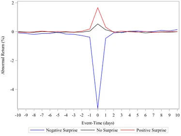
Figure 2 shows the stock market reaction to management earnings forecasts. Figure 2a looks at the average abnormal return for each day

in the [–10,+10] management earnings forecast event window. A clear

stock market reaction is discernible with an abnormal return of almost –6% on the day of the forecast for negative surprises and 2% for positive surprises. The asymmetric reaction is consistent with findings in the

(15)

literature. Figure 2b looks at the average cumulative abnormal return

for the subsequent [0,+60] earnings announcement event window. The

negative surprises, which experienced a large negative abnormal return on the day of the management earnings forecast, show a positive drift after the earnings announcement for an average cumulative abnormal return of almost 2% after two months. Positive surprises show a negative drift of almost –2%.

I examine the statistical significance of the abnormal returns in table 1. The results in this table echo what is obvious from figure 2. Negative sur-prises are associated with a –5.86% cumulative abnormal return around the management earnings forecast, and a reversal of 1.88% after the earnings announcement. Positive surprises are associated with a 1.93% cumulative abnormal return around the management earnings forecast, and a reversal of –1.72% after the earnings announcement. These abnor-mal returns are all statistically significant at the 1% level. No surprises show a pattern that is similar to that of positive surprises, but with a lower magnitude.

The robustness of the prior results is assessed in a multivariate regres-sion framework. Table 2 presents OLS regresregres-sions of the cumulative abnormal returns on control variables as well as firm and year fixed

effects. Specifically, I add the mean analyst forecast and management

earnings forecast to control for the level of expected earnings from both the analysts’ and managers’ point of view, respectively. I also control for the size of the firm and amount of coverage it receives using the number

(16)

of analysts following the firm in the past year. Finally, I control earn-ings uncertainty using book-to-market, prior standardized unexpected

earnings, and the size of the management earnings forecast range.4 The

t-statistics are calculated using heteroskedasticity consistent standard errors. Model 1 in columns 1 and 2 confirm the results from figure 2 and table 1. In particular, management earnings forecasts that are associated with negative surprises have a cumulative abnormal return of –6.23% and a reversal after the earnings announcement of 3.90%. Management earn-ings forecasts that are associated with positive surprises have a cumulative abnormal return of 3.05% and a reversal after the earnings announcement of –2.09%. I also test if the cumulative abnormal returns around the

management earnings forecasts affect the cumulative abnormal returns

after the earnings announcement directly in column 3 (Model 2). This

would provide evidence not only of semi-strong form market inefficiency,

but also weak form market inefficiency. Indeed, a management earnings

forecast cumulative abnormal return increase of 1% is associated with a subsequent correction of –0.39%, everything else being equal.

3.3 Regulation Fair Disclosure

Regulation Fair Disclosure (Reg-FD) was approved by the U.S. Securities and Exchange Commission on August 10, 2000. Reg-FD is intended to level the playing field by reducing information disparities between indi-vidual and institutional market participants (Bailey, Li, Mao, and Zhong,

(17)

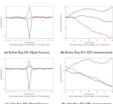
2003). Reg-FD prohibits selective disclosure of material information and requires broad, non-exclusionary disclosure of such information. I sepa-rate the sample into two sub-periods covering the years before and after Reg-FD in order to see what impact this regulation has had, if any, on the stock market reaction to management earnings forecasts. Figure 3 shows the stock market reaction to management earnings forecasts for each sub-period. Figures 3a and 3c look at the average abnormal return for

each day in the [–10,+10] management earnings forecast event window,

before and after Reg-FD, respectively. The stock market reaction before Reg-FD is about –10% on the day of the forecast for negative surprises and 5% for positive surprises. This is more than twice the size of the stock market reaction after Reg-FD, which is about –4% for negative surprises and 2% for positive surprises. Figures 3b and 3d look at the

average cumulative abnormal return for the subsequent [0,+60] earnings

announcement event window, before and after the passing of Reg-FD, respectively. Before Reg-FD, the negative surprises that are associated with a large negative abnormal return on the day of the management earnings forecast show a positive drift after the earnings announcement for an average cumulative abnormal return of about 5% after two months. After Reg-FD, this correction is just over 1%. Positive surprises show a negative drift of almost –10% before Reg-FD, and a negative drift of about –1.5% after.

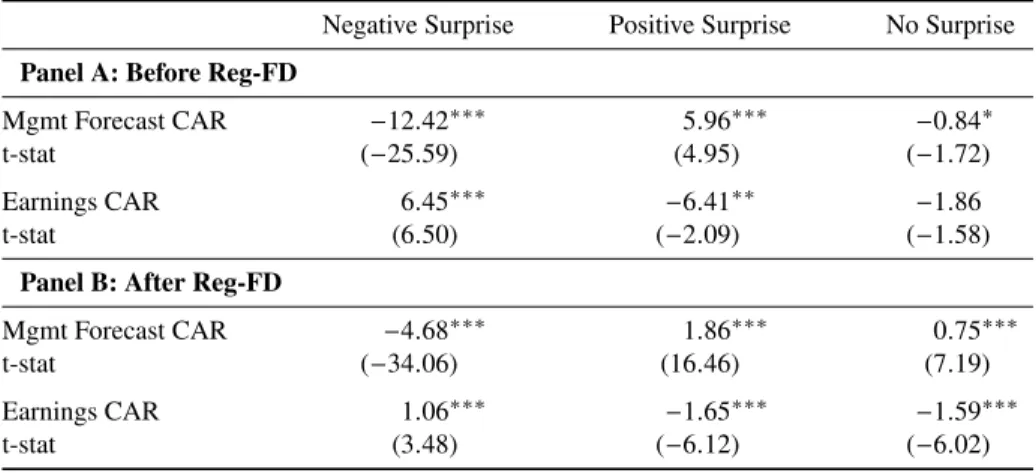
Table 3 reports the statistical significance of the abnormal returns. Before Reg-FD, negative surprises are associated with a –12.42%

(18)

cumu-lative abnormal return around the management earnings forecast, and a reversal of 6.45% after the earnings announcement. After Reg-FD, negative surprises are associated with a –4.68% cumulative abnormal return around the management earnings forecast, and a reversal of 1.06% after the earnings announcement. Before Reg-FD, positive surprises are associated with a 5.96% cumulative abnormal return around the man-agement earnings forecast, and a reversal of –6.41% after the earnings announcement. After Reg-FD, positive surprises are associated with a 1.86% cumulative abnormal return around the management earnings forecast, and a reversal of –1.65% after the earnings announcement. No surprises show no overreaction before Reg-FD. After Reg-FD,no sur-prises show a pattern that is similar to that of positive sursur-prises, but with a lower magnitude.

The robustness of the sub-period results is assessed in a multivariate regression framework. Table 4 presents OLS regressions of the cumula-tive abnormal returns on the control variables described above as well

as firm and year fixed effects. The t-statistics are calculated using

het-eroskedasticity consistent standard errors. The first three columns report results for the period before Reg-FD, while the last three columns report the results for the period after Reg-FD. Model 1 in columns 1 and 2 indicate that before Reg-FD, overreaction was mainly driven by nega-tive surprises. Management earnings forecasts that are associated with negative surprises have a cumulative abnormal return of –10.53% and a re-versal after the earnings announcement of 7.50%. Management earnings

(19)

forecasts that are associated with positive surprises have a cumulative abnormal return of 6.03%, but no reliable reversal after the earnings announcement. I also test if the cumulative abnormal returns around the

management earnings forecasts affect the cumulative abnormal returns

after the earnings announcement directly in column 3 (Model 2). A management earnings forecast cumulative abnormal return increase of 1% is associated with a subsequent correction of –0.20%. Model 1 in columns 4 and 5 indicate that after Reg-FD, overreaction occurs for both negative and positive surprises. Management earnings forecasts that are associated with negative surprises have a cumulative abnormal return of –5.88% and a reversal after the earnings announcement of 3.50%. Management earnings forecasts that are associated with positive surprises have a cumulative abnormal return of 2.96%, and a reversal after the earnings announcement of –1.91%. I also test if the cumulative abnormal

returns around the management earnings forecasts affect the cumulative

abnormal returns after the earnings announcement directly in column 3 (Model 6). A management earnings forecast cumulative abnormal return increase of 1% is associated with a subsequent correction of –0.41%.

The results in this subsection show that while the level of stock market overreaction was greater before Reg-FD, the marginal impact is greater after Reg-FD. Moreover, overreaction after Reg-FD is more balanced, in the sense that it occurs not only for negative surprises, but also for positive surprises.

(20)

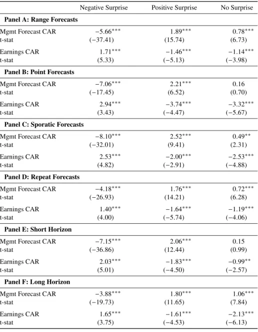
3.4 Management Forecast Characteristics

Management has discretion over certain aspects of the earnings forecasts they make. In particular, management can decide whether to issue a point forecast (i.e. one estimate) or a range forecast (i.e. a low and high estimate). In the literature, this is known as the forecast form. They can also decide whether to supply forecasts to market participants repeatedly or sporadically, and whether to provide a forecast early in the quarter or late in the quarter. The former is referred to as forecast frequency, while the latter is referred to as forecast timing. The impact of these forecast characteristics on stock market overreaction is examined in this subsection. The statistical significance of the abnormal returns by forecast form, frequency and timing is investigated in table 5. For range (point) forecasts, negative surprises are associated with a –5.66% (–7.06%) cu-mulative abnormal return around the management earnings forecast, and a reversal of 1.71% (2.94%) after the earnings announcement. The positive surprises of range (point) forecasts are associated with a 1.89% (2.21%) cumulative abnormal return around the management earnings forecast, and a reversal of –1.46% (–3.74%) after the earnings announcement. For sporadic (repeat) forecasts, negative surprises are associated with a –8.10% (–4.18%) cumulative abnormal return around the management earnings forecast, and a reversal of 2.53% (1.40%) after the earnings announcement. The positive surprises of sporadic (repeat) forecasts are associated with a 2.52% (1.76%) cumulative abnormal return around the

(21)

management earnings forecast, and a reversal of –2.00% (–1.64%) after the earnings announcement. Finally, for short (long) horizon forecasts, negative surprises are associated with a –7.15% (–3.88%) cumulative ab-normal return around the management earnings forecast, and a reversal of 2.03% (1.65%) after the earnings announcement. The positive surprises of short (long) horizon forecasts are associated with a 2.06% (1.80%) cumulative abnormal return around the management earnings forecast, and a reversal of –1.83% (–1.61%) after the earnings announcement.

I examine the robustness of the prior results in a multivariate regres-sion framework. Table 6 presents OLS regresregres-sions of the marginal impact of the cumulative abnormal return around the management earnings fore-cast on the cumulative abnormal return after the earnings announcement

and on control variables as well as firm and year fixed effects, for each

subsample separately. The control variables are the same as those used in table 2 and 4 regressions. The t-statistics are calculated using het-eroskedasticity consistent standard errors. Interestingly, the marginal impact of the stock market reaction to management earnings forecasts is fairly constant across subsamples. In particular, a management earnings forecast cumulative abnormal return increase of 1% is associated with a subsequent correction of between –0.38% and –0.44%, depending on the subsample.

The results in this subsection confirm that forecast characteristics do

not qualitatively affect the abnormal return pattern documented in the

(22)

sporadic forecasts and short horizon forecasts are all associated with more stock market overreaction than range forecasts, repeat forecasts and long horizon forecasts, respectively. Even though the level of stock market

reaction is different in different subsamples, the marginal impact of the

market’s initial reaction to management’s forecast barely changes.

3.5 Firm Characteristics

Firm characteristics may also impact the stock market overreaction. For example, small firms, growth firms and firm with low analyst coverage are all associated with greater uncertainty, and may therefore illicit a greater stock market reaction as a result. While I control for these firm characteristics in the table 2 and 4 regressions, the level of overreaction

may nevertheless be different in subsamples based on these characteristics.

The impact of firm characteristics on stock market overreaction is reported in this subsection. The statistical significance of the abnormal returns by firm size, book-to-market and analyst coverage is shown in table 7. For small (large) firms, negative surprises are associated with a –6.71% (–4.66%) cumulative abnormal return around the management earnings forecast, and a reversal of 2.54% (0.96%) after the earnings announce-ment. The positive surprises of small (large) firms are associated with a 2.78% (1.22%) cumulative abnormal return around the management earnings forecast, and a reversal of –1.16% (–2.18%) after the earnings announcement. For growth firms, negative surprises are not associated with any overreaction, but positive surprises are associated with a 2.01%

(23)

cumulative abnormal return around the management earnings forecast, and a reversal of –4.01% after the earnings announcement. The reverse is true of value firms. That is, positive surprises are not associated with any overreaction, but negative surprises are associated with a –5.22% cumulative abnormal return around the management earnings forecast, and a reversal of 3.48% after the earnings announcement. Finally, for low (high) analyst coverage firms, negative surprises are associated with a –6.38% (–5.18%) cumulative abnormal return around the management earnings forecast, and a reversal of 1.81% (2.05%) after the earnings an-nouncement. The positive surprises of low (high) analyst coverage firms are associated with a 2.60% (1.41%) cumulative abnormal return around the management earnings forecast, and a reversal of –2.39% (–1.17%) after the earnings announcement.

The prior results are reexamined in a multivariate regression frame-work. Table 8 presents OLS regressions of the marginal impact of the cumulative abnormal return around the management earnings forecast on the cumulative abnormal return after the earnings announcement and on

control variables as well as firm and year fixed effects, for each subsample

separately. The control variables are the same as those used in table 2, 4 and 6 regressions. The t-statistics are calculated using heteroskedasticity consistent standard errors. Again, the marginal impact of the stock mar-ket reaction to management earnings forecasts is fairly constant across subsamples. Specifically, a management earnings forecast cumulative abnormal return increase of 1% is associated with a subsequent correction

(24)

of between –0.40% and –0.43% depending on the subsample.

The results in this subsection show that small firms and low coverage firms are associated with more stock market overreaction than large firms and firms with high analyst coverage, respectively. The level of stock

market reaction is different in different subsamples, but the marginal

impact of the initial market reaction to management forecasts does not change materially. One notable finding in this subsection is that the stock market does not overreact to growth firms that announce bad news or to value firms that announce good news. If book-to-market captures

recent winners (low B/M) and losers (high B/M), it may be that the stock

market overreaction I document is related to the short-run continuation

and long-run return reversal patters found in the literature.5

3.6 Relative Analyst Forecasts

In this subsection, I examine whether the analyst forecasts given in re-sponse to the management earnings forecast impact the stock market reaction. Figures 4a and 4b show the distribution of relative analyst forecasts for range and point forecasts, respectively. The relative analyst forecast measure for range forecasts is the analyst forecast minus the midpoint of the management earnings forecast range, divided by the size of the forecast range. Analyst forecasts exactly equal to the management earnings forecast range low, mid and high points have a value of –0.5,

5_{Overreaction followed by undercorrection would lead to positive autocorrelation in the short-run, while} subsequent overreaction followed by overcorrection would lead to negative autocorrelation in the long-run.

(25)

0 and 0.5, respectively. A striking feature of this figure is that analysts predominantly issue forecasts equal to the management forecast range low, mid and high points. In fact, 85% of analyst forecasts are on the reference points for management earnings range forecasts. The relative analyst forecast measure for point forecasts is the analyst forecast minus the management earnings point forecast, divided by the the management earnings point forecast. Analyst forecasts exactly equal to the manage-ment earnings point forecast have a value of 0. This figure shows that the distribution of analyst forecasts for management earnings point forecasts is much less dispersed than for range forecasts. Nevertheless, analysts predominantly issue forecasts equal to the management point forecast. Indeed, 35% of analyst forecasts are exactly equal to the management earnings point forecast.

Given the above description of the analyst forecast distribution around management earnings forecasts, I create categorical variables to classify analyst forecasts relative to management forecasts as follows. For man-agement earnings range forecasts, analyst forecasts are either above the range high point (optimistic), at the range high point (cautiously opti-mistic), between the range high and low points (neutral), at the range low point (cautiously pessimistic), or below the range low point (pessimistic). For management earnings point forecasts, the number categories is re-duced to three (optimistic, neutral, or pessimistic). I then aggregate at the management forecast level. For management earnings range forecasts, an-alysts are considered optimistic, cautiously optimistic, neutral, cautiously

(26)

pessimistic, or pessimistic if all analysts on that day were in the same category. Otherwise, analyst forecasts are considered to be “mixed”. The same methodology is used with management earnings point forecasts.

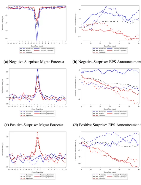
Figure 5 shows how relative analyst forecast impact stock market over-reaction for range forecasts. As one might expect when there is a negative surprise, all categories of relative analyst forecasts experience negative stock market reactions. However, cautiously pessimistic analyst forecasts experience much more negative reactions than the other four categories, with an abnormal return of about –8%. After the earnings announcement, cautiously pessimistic analyst forecasts also experience a more positive drift than the other four categories, with a correction of almost 4%. For positive surprises, all categories of relative analyst forecasts experience positive stock market reactions. There is little to distinguish the five categories, although cautiously pessimistic, neutral, and cautiously opti-mistic forecasts have slightly more positive reactions. However, after the earnings announcement, pessimistic, cautiously pessimistic and neutral analyst forecasts experience very little downward drift, while cautiously optimistic and optimistic analyst forecasts experience a more negative drift, with a correction of about –4%. Figure 6 shows how relative analyst forecast impact stock market overreaction for point forecasts. In terms of the stock market reaction to management earnings forecasts, neutral analyst forecasts appear to have the largest impact for both negative and positive surprises, although pessimistic and optimistic analyst forecasts also have strong stock market reactions. However, the subsequent stock

(27)

market correction shows a similar pattern for all three categories (i.e. positive corrections for negative surprises and negative corrections for positive surprises). Therefore, although the three categories mimic the trend for the overall sample of management earnings point forecasts, the

difference between them is slight.

The statistical significance of the abnormal returns by relative analyst forecast category is investigated in tables 9 and 10 for range and point forecasts, respectively. The results in table 9 are similar to those in fig-ure 5. For negative management forecast surprises, cautiously pessimistic and neutral analyst forecasts experience stock market overreaction, while the other three categories do not. Cautiously pessimistic (neutral) fore-casts are associated with management earnings forecast abnormal returns of –10.08% (–5.42%), and subsequent earnings announcement drift of 4.38% (1.66%). For positive management forecast surprises, neutral and cautiously optimistic analyst forecasts experience stock market overre-action, while the other three categories do not. Cautiously optimistic (neutral) forecasts are associated with management earnings forecast abnormal returns of 1.96% (2.03%), and subsequent earnings announce-ment drift of –2.68% (–1.68%). For point forecasts, the results in table 10 are more telling than those in figure 6. For negative surprises, neutral analyst forecasts are the only forecasts to experience overreaction, with an abnormal return of –8.93% and a subsequent correction of 3.26%. For positive surprises, neutral and optimistic analyst forecasts experi-ence overreaction, with an abnormal returns of 3.32% and 2.16%, and

(28)

subsequent corrections of –4.82% and –6.88%, respectively.

The evidence in this subsection shows that the stock market over-reaction found in this paper is present mainly when analyst forecasts corroborate management forecasts. Overreaction is also present when

there are mixed forecasts, suggesting that analyst disagreement is insu

ffi-cient to eliminate this anomaly. What is required to eliminate overreaction

is a clear analyst signal that is clear to investors, but different from

man-agement’s signal.

4 Conclusion

This paper examines whether the stock market overreacts to management earnings forecasts. I find that this is in fact the case for both positive and negative surprises, but more so for negative surprises. This overreaction still persists after the introduction of Regulation Fair Disclosure, although the level of the overreaction has decreased since this legislation was intro-duced. The level of stock market overreaction to management earnings forecasts changes depending on the forecast form, frequency and timing of management earnings forecasts, as well as the size, growth prospect and analyst coverage of the firm. However, the reaction to management earnings forecasts has almost the same marginal impact on the subse-quent reaction to earnings announcement, regardless of the forecast or firm characteristic examined. I also investigate whether analyst forecasts

(29)

market reaction. Return reversals appear strongest in situations when analysts provide confirmatory forecasts in response to the management earnings forecast. This evidence is consistent with the idea that in situa-tion of increased uncertainty, behavioral biases may cause investors to overweight their recent investment experience, leading to stock market overreaction.

This paper has implications in terms of information dissemination

and its impact on market efficiency. The results show that the

imple-mentation of Regulation Fair Disclosure has helped to reduce the level of stock market overreaction to management forecasts, suggesting that

a even playing field does improve informational efficiency. Through

their forecasts, analysts appear to have the power to reduce stock market reaction even further. For the most part however, analysts provide incre-mentally uninformative forecasts in the sense that their forecasts are not

(30)

References

Abarbanell, J.S., and V.L. Bernard, 1992, Tests of analysts’ overreaction/

underreaction to earnings information as an explanation for anomalous stock price behavior, Journal of Finance 47, 1181–1207.

Bailey, W., H. Li, C.X. Mao, and R. Zhong, 2003, Regulation fair dis-closure and earnings information: Market, analyst, and corporate re-sponses, Journal of Finance 58, 2487–2514.

Ball, R., and P. Brown, 1968, An empirical evaluation of accounting income numbers, Journal of Accounting Research 6, 159–178.

Ball, R., and S.P. Kothari, 1989, Nonstationary expected returns:

Impli-cations for tests of market efficiency and serial correlation in returns,

Journal of Financial Economics25, 673–717.

Barberis, N., A. Shleifer, and R. Vishny, 1998, A model of investor sentiment, Journal of Financial Economics 49, 307–343.

Bekaert, G., and G. Wu, 2000, Asymmetric volatility and risk in equity markets, Review of Financial Studies 13, 1–42.

Campbell, J.Y., and L. Hentschel, 1992, No news is good news: An asymmetric model of changing volatility in stock returns, Journal of

Financial Economics31, 565–590.

Chan, K.C., 1988, On the contrarian investment strategy, Journal of

(31)

Chan, W.S., 2003, Stock price reaction to news and no-news: Drift and reversal after headlines, Journal of Financial Economics 70, 223–260. Chopra, N., J. Lakonishok, and J.R. Ritter, 1992, Measuring abnormal

performance, Journal of Financial Economics 31, 235–268.

Cooper, I., and R. Priestley, 2011, Real investment and risk dynamics,

Cooper, M.J., H. Gulen, and M.J. Schill, 2008, Asset growth and the cross-section of stock returns, Journal of Finance 63, 1609–1651. Cotter, J., I. Tuna, and P.D. Wysocki, 2006, Expectations management and

beatable targets: How do analysts react to explicit earnings guidance?,

Contemporary Accounting Research23, 593–624.

Cutler, D.M., J.M. Poterba, and L.H. Summers, 1991, Speculative dy-namics, Review of Economic Studies 58, 529–546.

Daniel, K., D. Hirshleifer, and A. Subrahmanyam, 1998, Investor psychol-ogy and security market under- and overreactions, Journal of Finance 53, 1839–1885.

De Bondt, W., and R. Thaler, 1985, Does the stock market overreact?,

Journal of Finance40, 793–805.

, 1987, Further evidence on investor overreaction and stock market seasonality, Journal of Finance 42, 557–581.

(32)

Debondt, W.F.M., and R.H. Thaler, 1990, Do security analysts overreact?,

American Economic Review80, 52–57.

Easterwood, J.C., and S.R. Nutt, 1999, Inefficiency in analysts’ earnings

forecasts: Systematic misreaction or systematic optimism?, Journal of

Finance54, 1777–1797.

Fama, E.F., and K.R. French, 1988, Permanent and temporary compo-nents of stock prices, Journal of Political Economy 96, 246–273.

, 1993, Common risk factors in the returns on stocks and bonds,

Foster, G., C. Olsen, and T. Shevlin, 1984, Earnings releases, anomalies, and the behavior of security returns, Accounting Review 59, 574–859. French, K.R., G.W. Schwert, and R.F. Stambaugh, 1987, Expected stock

returns and volatility, Journal of Financial Economics 19, 3–29. George, T.J., and C.-Y. Hwang, 2007, Long-term return reversals:

Over-reaction or taxes?, Journal of Financial Finance 62, 2865–2896. Hirshleifer, D., 2001, Investor psychology and asset pricing, Journal of

Finance56, 1533–1597.

Hirst, D.E., L. Koonce, and S. Venkataraman, 2008, Management earn-ings forecasts:a review and framework, Accounting Horizons 22, 315– 338.

(33)

Hong, H., and J.D. Kubik, 2003, Analyzing the analysts: Career concerns and biased earnings forecasts, Journal of Finance 58, 313–351.

Hong, H., and J.C. Stein, 1999, A unified theory of underreaction, mo-mentum trading, and overreaction in asset markets, Journal of Finance 54, 2143–2184.

Hughes, J., and S. Pae, 2004, Voluntary disclosure of precision informa-tion, Journal of Accounting and Economics 37, 261–289.

Jackson, A.R., 2005, Trade generation, reputation, and sell-side analysts,

Jiang, G., C.M.C. Lee, and Y. Zhang, 2005, Information uncertainty and expected returns, Review of Accounting Studies 10, 185–221.

King, R., G. Pownall, and G. Waymire, 1990, Expectations adjustments via timely management forecasts: Review, synthesis, and suggestions for future research, Journal of Accounting Literature 9, 113–144.

Klein, P., 2001, The capital gain lock-in effect and long-horizon return

reversal, Journal of Financial Economics 59, 33–62.

Ko, J.K., and Z. Huang, 2007, Arrogance can be a virtue: Overconfidence,

information acquisition, and market efficiency, Journal of Financial

Economics84, 529–560.

Kothari, S.P., S. Shu, and P.D. Wysocki, 2009, Do managers withhold bad news?, Journal of Accounting Research 47, 241–276.

(34)

La Porta, R., 1996, Expectations and the cross-section of stock returns,

, J. Lakonishok, A. Shleifer, and R.W. Vishny, 1997, Good news

for value stocks: Further evidence on market efficiency, Journal of

Finance52, 859–874.

Lakonishok, J., A. Shleifer, and R.W. Vishny, 1994, Contrarian invest-ment, extrapolation, and risk, Journal of Finance 49, 1541–1578. Lim, T., 2001, Rationality and analysts’ forecast bias, Journal of Finance

56, 369–385.

Patell, J.M., 1976, Corporate forecasts of earnings per share and stock price behavior: Empirical test, Journal of Accounting Research 14, 246–276.

Penman, S.H., 1980, An empirical investigation of the voluntary disclo-sure of corporate earnings forecasts, Journal of Accounting Research 18, 132–160.

Pindyck, R.S., 1984, Risk, inflation, and the stock market, American

Economic Review74, 335–351.

Poterba, J.M., and L.H. Summers, 1988, Mean reversion in stock prices,

Rogers, J.L., D.J. Skinner, and A. Van Buskirk, 2009, Earnings guidance and market uncertainty, Journal of Accounting and Economics 48, 90–109.

(35)

Tetlock, P.C., 2011, All the news that’s fit to reprint: Do investors react to stale information?, Review of Financial Studies 24, 1481–1512. Tversky, A., and D. Kahneman, 1974, Judgment under uncertainty:

Heuristics and biases, Science 185, 1124–1131.

Wu, G., 2001, The determinants of asymmetric volatility, Review of

Financial Studies14, 837–859.

Zarowin, P., 1990, Size, seasonality, and stock market overreaction,

Jour-nal of Financial and Quantitative AJour-nalysis25, 113–125.

Zhang, X.F., 2006a, Information uncertainty and analyst forecast behavior,

Contemporary Accounting Research23, 565–590.

, 2006b, Information uncertainty and stock returns, Journal of

(36)

199₄199₅199₆ 199₇199₈ 199₉200₀200₁200₂200₃200₄ 200₅200₆ 200₇ 200₈200₉201₀201₁ Year 0 2000 4000 6000 8000 10000 12000 F re qu en cy Positive Surprise No Surprise Negative Surprise

Figure 1: Yearly Frequency of Management Forecasts by Forecast Surprise

This figure reports the yearly frequency of management forecasts by the type of surprise which the forecast represents. A Negative Surprise occurs when the management forecast estimate is below the current analyst forecast consensus. No Surprise occurs when the management forecast estimate is equal to the current analyst forecast consensus. A Positive Surprise occurs when the management forecast estimate is above the current analyst forecast consensus.

(37)

-10 -9 -8 -7 -6 -5 -4 -3 -2 -1 0 1 2 3 4 5 6 7 8 9 10 Event-Time (days) -4 -2 0 2 A bn or m al R et ur n ( % ) Positive Surprise No Surprise Negative Surprise (a) Mgmt Forecast 0 10 20 30 40 50 60 Event-Time (days) -2 -1 0 1 2 C um ul at iv e A bn or m al R et ur n ( % ) Positive Surprise No Surprise Negative Surprise (b) EPS Announcement

Figure 2: Management Forecast Average Abnormal Returns

This figure reports the average abnormal return for the [-10,+10] management forecast window (Mgmt Forecast) and average cumulative abnormal returns for the subsequent [0,+60] earnings announcement window (EPS Announcement) for various subsamples. A Negative Surprise occurs when the management forecast estimate is below the current analyst forecast consensus. No Surprise occurs when the management forecast estimate is equal to the current analyst forecast consensus. A Positive Surprise occurs when the management forecast estimate is above the current analyst forecast consensus. Abnormal return is calculated using a Fama-French 3-factor model to estimate the expected return.

(38)

-10 -9 -8 -7 -6 -5 -4 -3 -2 -1 0 1 2 3 4 5 6 7 8 9 10 Event-Time (days) -10 -5 0 5 A bn or m al R et ur n ( % ) Positive Surprise No Surprise Negative Surprise

(a) Before Reg-FD: Mgmt Forecast

0 10 20 30 40 50 60 Event-Time (days) -10 -5 0 5 C um ul at iv e A bn or m al R et ur n ( % ) Positive Surprise No Surprise Negative Surprise

(b) Before Reg-FD: EPS Announcement

-10 -9 -8 -7 -6 -5 -4 -3 -2 -1 0 1 2 3 4 5 6 7 8 9 10 Event-Time (days) -4 -2 0 2 A bn or m al R et ur n ( % ) Positive Surprise No Surprise Negative Surprise

(c) After Reg-FD: Mgmt Forecast

0 10 20 30 40 50 60 Event-Time (days) -2 -1 0 1 C um ul at iv e A bn or m al R et ur n ( % ) Positive Surprise No Surprise Negative Surprise

(d) After Reg-FD: EPS Announcement

Figure 3: Management Forecast Average Abnormal Returns by Subperiod

This figure reports the average abnormal return for the [-10,+10] management forecast window (Mgmt Forecast) and average cumulative abnormal returns for the subsequent [0,+60] earnings announcement window (EPS Announcement) for various subsamples. Before Reg-FD refers to the calendar period up until the year 2000, while After Reg-FD refers to the calendar period after the year 2000. A Negative Surprise occurs when the management forecast estimate is below the current analyst forecast consensus. No Surprise occurs when the management forecast estimate is equal to the current analyst forecast consensus. A Positive Surprise occurs when the management forecast estimate is above the current analyst forecast consensus. Abnormal return is calculated using a Fama-French 3-factor model to estimate the expected return.

(39)

-2.0 -1.5 -1.0 -0.5 0.0 0.5 1.0 1.5 2.0 Analyst Forecasts Relative to Management Forecasts

0 5 10 15 20 25 P er ce nt

(a) Range Forecast

-2.0 -1.5 -1.0 -0.5 0.0 0.5 1.0 1.5 2.0

Analyst Forecasts Relative to Management Forecasts 0 20 40 60 80 100 P er ce nt (b) Point Forecast

Figure 4: Distribution of Analyst Forecasts Relative to Management Forecasts

This figure reports the percentage frequency distribution of analyst forecasts relative to the management forecast. The relative measure for range forecasts in figure (a) is the Analyst Forecast minus the management forecast range midpoint, divided by the management forecast range high point minus the low point. The relative measure for point forecasts in figure (b) is the Analyst Forecast minus the management forecast, divided by the management forecast. Analyst Forecast is the analyst quarterly EPS forecast.

(40)

-10 -9 -8 -7 -6 -5 -4 -3 -2 -1 0 1 2 3 4 5 6 7 8 9 10 Event-Time (days) -8 -6 -4 -2 0 A bn or m al R et ur n ( % )

Optimistic Cautiously Optimistic

Neutral Cautiously Pessimistic

Pessimistic

(a) Negative Surprise: Mgmt Forecast

0 10 20 30 40 50 60 Event-Time (days) -2 0 2 4 C um ul at iv e A bn or m al R et ur n ( % )

Pessimistic

(b) Negative Surprise: EPS Announcement

-10 -9 -8 -7 -6 -5 -4 -3 -2 -1 0 1 2 3 4 5 6 7 8 9 10 Event-Time (days) -0.5 0.0 0.5 1.0 1.5 2.0 A bn or m al R et ur n ( % )

Pessimistic

(c) Positive Surprise: Mgmt Forecast

0 10 20 30 40 50 60 Event-Time (days) -4 -2 0 2 C um ul at iv e A bn or m al R et ur n ( % )

Pessimistic

(d) Positive Surprise: EPS Announcement

-10 -9 -8 -7 -6 -5 -4 -3 -2 -1 0 1 2 3 4 5 6 7 8 9 10 Event-Time (days) -0.5 0.0 0.5 1.0 A bn or m al R et ur n ( % )

Pessimistic

(e) No Surprise: Mgmt Forecast

0 10 20 30 40 50 60 Event-Time (days) -3 -2 -1 0 1 C um ul at iv e A bn or m al R et ur n ( % )

Pessimistic

(f) No Surprise: EPS Announcement

Figure 5: Management Range Forecast Average Abnormal Returns by Relative Analyst Forecast

This figure reports the average abnormal return for the [-10,+10] management forecast window (Mgmt Forecast) and average cumulative abnormal returns for the subsequent [0,+60] earnings announcement window (EPS Announcement) for various subsamples. A Negative Surprise occurs when the management forecast estimate is below the current analyst forecast consensus. No Surprise occurs when the management forecast estimate is equal to the current analyst forecast consensus. A Positive Surprise occurs when the management forecast estimate is above the current analyst forecast consensus. Pessimistic is day on which all analyst forecasts of quarterly EPS are less than the management forecast low point. Cautiously Pessimistic is a day on which all analyst forecasts of quarterly EPS are equal to the management forecast low point. Neutral is a day on which all analyst forecasts of quarterly EPS are between the management forecast low and high points. Cautiously Optimistic is a day on which all analyst forecasts of quarterly EPS are equal to the management forecast high point. Optimistic is a day on which all analyst forecasts of quarterly EPS are

(41)

-10 -9 -8 -7 -6 -5 -4 -3 -2 -1 0 1 2 3 4 5 6 7 8 9 10 Event-Time (days) -8 -6 -4 -2 0 A bn or m al R et ur n ( % ) Optimistic Neutral Pessimistic

(a) Negative Surprise: Mgmt Forecast

0 10 20 30 40 50 60 Event-Time (days) 0 2 4 6 C um ul at iv e A bn or m al R et ur n ( % ) Optimistic Neutral Pessimistic

(b) Negative Surprise: EPS Announcement

-10 -9 -8 -7 -6 -5 -4 -3 -2 -1 0 1 2 3 4 5 6 7 8 9 10 Event-Time (days) 0 1 2 3 A bn or m al R et ur n ( % ) Optimistic Neutral Pessimistic

(c) Positive Surprise: Mgmt Forecast

0 10 20 30 40 50 60 Event-Time (days) -6 -4 -2 0 C um ul at iv e A bn or m al R et ur n ( % ) Optimistic Neutral Pessimistic

(d) Positive Surprise: EPS Announcement

-10 -9 -8 -7 -6 -5 -4 -3 -2 -1 0 1 2 3 4 5 6 7 8 9 10 Event-Time (days) -1.0 -0.5 0.0 0.5 A bn or m al R et ur n ( % ) Optimistic Neutral Pessimistic

(e) No Surprise: Mgmt Forecast

0 10 20 30 40 50 60 Event-Time (days) -4 -2 0 C um ul at iv e A bn or m al R et ur n ( % ) Optimistic Neutral Pessimistic

(f) No Surprise: EPS Announcement

Figure 6: Management Point Forecast Average Abnormal Returns by Relative Analyst Forecast

This figure reports the average abnormal return for the [-10,+10] management forecast window (Mgmt Forecast) and average cumulative abnormal returns for the subsequent [0,+60] earnings announcement window (EPS Announcement) for various subsamples. A Negative Surprise occurs when the management forecast estimate is below the current analyst forecast consensus. No Surprise occurs when the management forecast estimate is equal to the current analyst forecast consensus. A Positive Surprise occurs when the management forecast estimate is above the current analyst forecast consensus. Pessimistic is day on which all analyst forecasts of quarterly EPS are less than the management forecast. Neutral is a day on which all analyst forecasts of quarterly EPS are equal to the management forecast. Optimistic is a day on which all analyst forecasts of quarterly EPS are greater than the management forecast. Abnormal return is calculated using a Fama-French 3-factor model to estimate the expected return.

(42)

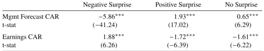
Table 1: Management Forecast Abnormal Returns

This table reports the management forecast average 3-day cumulative abnormal returns (Mgmt Forecast CAR) and subsequent earnings announcemet average 61-day cumulative abnormal returns (Earnings CAR), in percentage on various subsamples. A Negative Surprise occurs when the management forecast estimate is below the current analyst forecast consensus. No Surprise occurs when the management forecast estimate is equal to the current analyst forecast consensus. A Positive Surprise occurs when the management forecast estimate is above the current analyst forecast consensus. Abnormal return is calculated using a Fama-French 3-factor model to estimate the expected return. The numbers in parentheses are simple t-statistics. ***, ** or * signify that the test statistic is significant at the 1, 5 or 10% two-tailed level, respectively.

Negative Surprise Positive Surprise No Surprise

Mgmt Forecast CAR −5.86∗∗∗ 1.93∗∗∗ 0.65∗∗∗

t-stat (−41.24) (17.02) (6.29)

Earnings CAR 1.88∗∗∗ −1.72∗∗∗ −1.61∗∗∗

(43)

Table 2: Management Forecast Abnormal Return Multivariate Regressions

This table reports the coefficients from a regression of management forecast 3-day cumulative abnormal returns (Mgmt Forecast CAR) and subsequent earnings announcemement 61-day cumulative abnormal returns (Earnings CAR) on multiple variables. A Negative Surprise occurs when the management forecast estimate is below the current analyst forecast consensus. A Positive Surprise occurs when the management forecast estimate is above the current analyst forecast consensus. Mean Analyst Forecast is the average analyst quarterly EPS forecast on the event day. Mgmt Forecast is the forecast point or middle point of the management quarterly EPS forecast range. Range is the difference between the Mgmt Forecast high and low points, divided by the stock price at the end of the prior month. Market Cap is the number of shares outstanding multiplied by the price, in millions of dollars. Book-to-Market is the book value of common equity divided by the market capitalization. Analyst Coverage is the number of analysts that have provided an EPS forecast for the firm over the past year. SUE is the ratio of the quarterly earnings surprise to the standard deviation of earnings surprises over the past four quarters. Abnormal return is calculated using a Fama-French 3-factor model to estimate the expected return. The numbers in parentheses are t-statistics based on heteroscedasticity consistent standard errors. ***, ** or * signify that the test statistic is significant at the 1, 5 or 10% two-tailed level, respectively.

Mgmt Forecast CAR Earnings CAR

Model 1 Model 1 Model 2

Mgmt Forecast CAR −0.39∗∗∗ (−23.50) Negative Surprise −6.23∗∗∗ 3.90∗∗∗ (−32.10) (8.64) Positive Surprise 3.05∗∗∗ −2.09∗∗∗ (13.40) (−3.94)

Mean Analyst Forecast 3.07∗∗∗ −1.22 −0.22

(4.07) (−0.70) (−0.13) Mgmt Forecast −0.98 2.51 1.79 (−1.38) (1.52) (1.09) Range 0.18 2.77∗∗∗ 2.94∗∗∗ (0.72) (4.75) (5.11) Ln(Market Cap) −3.89∗∗∗ −13.75∗∗∗ −15.26∗∗∗ (−19.00) (−28.88) (−32.15) Book-to-Market −0.02 −0.02 −0.02 (−0.76) (−0.23) (−0.31) Analyst Coverage 0.07∗∗∗ 0.49∗∗∗ 0.53∗∗∗ (3.13) (8.94) (9.86) SUE 0.07∗∗∗ −0.07∗∗∗ −0.04∗∗∗ (10.47) (−4.36) (−2.81) Intercept 44.24∗∗∗ 159.41∗∗∗ 176.59∗∗∗ (11.32) (17.53) (19.59) Adj. R2(%) 21.1 12.7 14.8 N 19,869 19,868 19,868

Firm Fixed Effects Y Y Y

(44)

Table 3: Management Forecast Abnormal Returns by Subperiod

This table reports the management forecast average 3-day cumulative abnormal returns (Mgmt Forecast CAR) and subsequent earnings announcemet average 61-day cumulative abnormal returns (Earnings CAR), in percentage on various subsamples. Before Reg-FD refers to the calendar period up until the year 2000, while After Reg-FD refers to the calendar period after the year 2000. A Negative Surprise occurs when the management forecast estimate is below the current analyst forecast consensus. No Surprise occurs when the management forecast estimate is equal to the current analyst forecast consensus. A Positive Surprise occurs when the management forecast estimate is above the current analyst forecast consensus. Abnormal return is calculated using a Fama-French 3-factor model to estimate the expected return. The numbers in parentheses are simple t-statistics. ***, ** or * signify that the test statistic is significant at the 1, 5 or 10% two-tailed level, respectively.

Panel A: Before Reg-FD

Mgmt Forecast CAR −12.42∗∗∗ 5.96∗∗∗ −0.84∗

t-stat (−25.59) (4.95) (−1.72)

Earnings CAR 6.45∗∗∗ −6.41∗∗ −1.86

t-stat (6.50) (−2.09) (−1.58)

Panel B: After Reg-FD

t-stat (−34.06) (16.46) (7.19)

Earnings CAR 1.06∗∗∗ −1.65∗∗∗ −1.59∗∗∗

(45)

T able 4: Management F or ecast Abnormal Retur n Multi v ariate Regr essions by Subperiod This table reports the coe ffi cients from a re gression of management forecast 3-day cumulati v e abnormal returns (Mgmt F orecast CAR) and subsequent earnings announcemement 61-day cumulati v e abnormal returns (Earnings CAR) on multiple v ariables. Before Re g-FD refers to the calendar period up until the year 2000, while After Re g-FD refers to the calendar period after the year 2000. A Ne g ati v e Surprise occurs when the management forecast estimate is belo w the current analyst forecast consensus. A Positi v e Surprise occurs when the management forecast estimate is abo v e the current analyst forecast consensus. Mean Analyst F orecast is the av erage analyst quarterly EPS forecast on the ev ent day . Mgmt F orecast is the forecast point or middle point of the management quarterly EPS forecast range. Range is the di ff erence between the Mgmt F orecast high and lo w points, di vided by the stock price at the end of the prior month. Mark et Cap is the number of shares outstanding multiplied by the price, in millions of dollars. Book-to-Mark et is the book v alue of common equity di vided by the mark et capitalization. Analyst Co v erage is the number of analysts that ha v e pro vided an EPS forecast for the firm o v er the past year . SUE is the ratio of the quarterly earnings surprise to the standard de viation of earnings surprises o v er the past four quarters. Abnormal return is calculated using a F ama-French 3-f actor model to estimate the expected return. The numbers in parentheses are t-statistics based on heteroscedasticity consistent standard errors. ***, ** or * signify that the test statistic is significant at the 1, 5 or 10% tw o-tailed le v el, respecti v ely . Before Re g-FD After Re g-FD Mgmt F orecast CAR Earnings CAR Mgmt F orecast CAR Earnings CAR Model 1 Model 2 Model 1 Model 2 Mgmt F orecast CAR − 0 .20 ∗ − 0 .41 ∗ ∗ ∗ (− 1 .89) (− 23 .65) Ne g ati v e Surprise − 10 .53 ∗ ∗ ∗ 7 .50 ∗ ∗ − 5 .88 ∗ ∗ ∗ 3 .50 ∗ ∗ ∗ (− 8 .27) (2 .32) (− 29 .92) (7 .60) Positi v e Surprise 6 .03 ∗ ∗ ∗ − 7 .23 2 .96 ∗ ∗ ∗ − 1 .91 ∗ ∗ ∗ (2 .87) (− 1 .36) (13 .02) (− 3 .60) Mean Analyst F orecast 7 .61 ∗ − 8 .19 − 8 .68 2 .54 ∗ ∗ ∗ − 0 .51 0 .39 (1 .74) (− 0 .74) (− 0 .78) (3 .23) (− 0 .28) (0 .22) Mgmt F orecast − 6 .44 0 .66 − 1 .08 − 0 .64 2 .28 1 .74 (− 1 .49) (0 .06) (− 0 .10) (− 0 .85) (1 .31) (1 .01) Range 1 .60 12 .79 13 .67 ∗ 0 .12 2 .68 ∗ ∗ ∗ 2 .81 ∗ ∗ ∗ (0 .51) (1 .59) (1 .70) (0 .48) (4 .54) (4 .84) Ln(Mark et Cap) − 5 .16 ∗ ∗ ∗ − 16 .41 ∗ ∗ ∗ − 18 .06 ∗ ∗ ∗ − 4 .06 ∗ ∗ ∗ − 14 .76 ∗ ∗ ∗ − 16 .41 ∗ ∗ ∗ (− 4 .38) (− 5 .48) (− 5 .96) (− 18 .78) (− 29 .18) (− 32 .54) Book-to-Mark et − 0 .30 0 .36 − 0 .51 − 0 .03 − 0 .04 − 0 .05 (− 0 .28) (0 .13) (− 0 .18) (− 1 .00) (− 0 .60) (− 0 .74) Analyst Co v erage − 0 .01 0 .17 0 .31 0 .09 ∗ ∗ ∗ 0 .53 ∗ ∗ ∗ 0 .58 ∗ ∗ ∗ (− 0 .05) (0 .37) (0 .68) (3 .65) (9 .31) (10 .26) SUE − 0 .28 ∗ 0 .11 − 0 .09 0 .08 ∗ ∗ ∗ − 0 .07 ∗ ∗ ∗ − 0 .04 ∗ ∗ (− 1 .76) (0 .28) (− 0 .21) (11 .10) (− 4 .32) (− 2 .55) Intercept 30 .35 205 .12 ∗ ∗ ∗ 223 .68 ∗ ∗ ∗ 55 .08 ∗ ∗ ∗ 195 .11 ∗ ∗ ∗ 216 .79 ∗ ∗ ∗ (1 .61) (4 .28) (4 .67) (16 .37) (24 .76) (27 .70) Adj. R 2(%) 52.7 20.2 19.3 15.7 11.2 13.6 N 1,349 1,349 1,349 18,520 18,519 18,519 Firm Fix ed E ff ects Y Y Y Y Y Y Y ear Fix ed E ff ects Y Y Y Y Y Y

(46)

Table 5: Management Forecast Abnormal Returns by Forecast Characteristic

This table reports the management forecast average 3-day cumulative abnormal returns (Mgmt Forecast CAR) and subsequent earnings announcemet average 61-day cumulative abnormal returns (Earnings CAR), in percentage on various subsamples. For Repeat Forecasts, management has provided at least three other forecasts in the past four quarters. Otherwise, forecasts are Sporatic Forecasts. A Short Horizon forecast is a forecast given within 60 days of the fiscal period end date. Otherwise, the forecast has a Long Horizon. A Negative Surprise occurs when the management forecast estimate is below the current analyst forecast consensus. No Surprise occurs when the management forecast estimate is equal to the current analyst forecast consensus. A Positive Surprise occurs when the management forecast estimate is above the current analyst forecast consensus. Abnormal return is calculated using a Fama-French 3-factor model to estimate the expected return. The numbers in parentheses are simple t-statistics. ***, ** or * signify that the test statistic is significant at the 1, 5 or 10% two-tailed level, respectively.

Panel A: Range Forecasts

t-stat (−37.41) (15.74) (6.73)

Earnings CAR 1.71∗∗∗ −1.46∗∗∗ −1.14∗∗∗

t-stat (5.33) (−5.13) (−3.98)

Panel B: Point Forecasts

Mgmt Forecast CAR −7.06∗∗∗ 2.21∗∗∗ 0.16

t-stat (−17.45) (6.52) (0.70)

Earnings CAR 2.94∗∗∗ −3.74∗∗∗ −3.32∗∗∗

t-stat (3.43) (−4.47) (−5.67)

Panel C: Sporatic Forecasts

Mgmt Forecast CAR −8.10∗∗∗ 2.52∗∗∗ 0.49∗∗

t-stat (−32.01) (9.41) (2.31)