Design and analysis of the ICRF antenna with active cooling

Design and Analysis of the ICRF Antenna

With Active Cooling

by

Dwight D. Caldwell

B.S. Mechanical Engineering, University of Waterloo (1988)

Submitted to the Department of Aeronautics and Astronautics in partial fulfillment of the requirements for the degree of

MASTER OF SCIENCE IN AERONAUTICS AND ASTRONAUTICS at the

Massachusetts Institute of Technology

September 1991

o Massachusetts Institute of Technology 1991 All rights reserved

Signature of Author

Department of Aeronautics and Astronautics SeDtember 1991

Certified by

Professor Miklos Porkolab Professor of Physics, Thesis Supervisor

Certified by _____

Professor 1Aniel Hastings Associate Professor of Aeronautics and Astronautics

Accepted by ...

PrQ'ssor Harold Y. Wachman

Chairman, Depa tment Graduate Committee

MASSACHUSETTS INSTITUTE OF TECHNOLOGY

SEP

2

4.

1991

UBRARIES

.-Design and Analysis of the ICRF Antenna

With Active Cooling

by

Dwight D. Caldwell

Submitted to the Department of Aeronautics and Astronautics on August 26, 1991 in partial fulfillment of the

requirements for the Degree of Master of Science in Aeronautics and Astronautics

ABSTRACT

A thermal finite element analysis was performed for the rf

antenna of the Alcator C-MOD tokamak. Alcator will be used for experimental tests on plasma which may lead to the harnessing of fusion power. The rf antenna will heat up as it emits electro-magnetic waves into the plasma. Pulses of at least 10 seconds duration were simulated followed by a twenty minute cooling period. The cooling effectiveness of liquid water, nitrogen gas, and no active cooling (radiation only) was tested and compared for the antenna.

The maximum pulse length without active cooling should not exceed 12 seconds when the tokamak is run for an eight hour day. The pulse length should be limited to 25 seconds with nitrogen cooling although the antenna will be cooled to its original temperature following the cooling period. Liquid water cooling would allow a pulse of indefinite length assuming that the tokamak walls do not heat to excessive temperatures. If the pulse is to be limited to under 12 seconds, then active cooling is not required, assuming that structural demands are met.

The use of rf heating as a means of propulsion was also examined. The tandem mirror rocket would expel a controlled amount of heated plasma in order to maintain a small constant

acceleration for a long period of time. In this way, the plasma rocket could be more fuel efficient and take less travel time for interplanetary voyages. The promise of full fusion powered

spacecraft was also explored for both interplanetary and interstellar journeys.

Thesis Supervisor: Professor Miklos Porkolab

Acknowledgements

For his support and guidance in the progress of this report, I would like thank my friend, Yuichi Takase. I would also like to express my appreciation to my advisors, Professor Porkolab and Professor Hastings, and to Dr. Yang, for making it possible for me to work on this project.

Table of Contents

1. Introduction ... 2. The Fusion Rocket

2.1 Fusion Rocket Performance

3. The Tandem Mirror Rocket ...

3.1 Antenna Cooling Analysis 3.2 Ideal Tandem Mirror Rocket 4. The Alcator C-MOD Tokamak

4.1 The RF Antenna ...

5. The Finite Element Model ... 5.1 Loading ...

5.2 Two-Dimensional Modelling

5.3 Faraday Shield Parameters

a5-... ee...e*0

Performance

Strategy ...

646406494096

5.3.2 Conduction ...

5.3.3 Convection ...

5.3.4 Faraday Shield Transverse Heat

5.4 Fluid Flow Elements ...

5.5 Faraday Shield Support Parameters 5.6 Solid Rod Properties ... 5.7 Radiation ... ...

5.8 Heat Loading ... ... 6. Material Properties ...

6.1 Convection Heat Transfer Coefficie 6.1.1 Laminar Flow ... 6.1.2 Turbulent Flow ... 6.2 Model Properties ... 7. Results ...0 .... ... 7.1 No Active Cooling ...

7.1.1

7.1.2

7.1.3

Radiation Cooling Effect Extended Pulse Length

Stress Evaluation ...

0000

0000

7.2 Active Cooling With Water

...

83

9 10 12 16 21 24 29 29 33 35 38 40 40 41 42 43 46 47 48 49 50 51 52 52 53 53 57 58 68 77 80 Flow 00000 oooe.0000 00000 00000 ooooo nt ... 00 00000 .0... 00... 0.0o. .... 0 nt . ...

7.3 Active Cooling With Nitrogen ... 91

8. Results Verification ... ... 97

8.1 Temperature Results

...

.

97

8.2 Three-Dimensional Model ... 100

8.2.1 Three-Dimensional Results Comparison ... 100

8.3 Radiation Check ... 1.g.

113

10. Conclusions and Recommendations ... 120

11. References ... ... .. .... .... .. 122

List of Figures

Plasma Flow ... ..

Magnetic Coil Configuration ....

Magnetic Field and Electric Field .... O. .. 600*0000

ICRF Antenna Schematic Diagram ... Antenna Model and Parameters ...

Variable and Constant Ip Rocket Comparison ... Variable and Constant Ip Rocket Voyage Profiles .. RF Antenna Assembly ... ... .. .,.. .

Torus Plasma Parameters .... ... RF Antenna Finite Element Model ... Pulse Input Power ...

Antenna Loading ... Equivalent Model ... Temperature Profile Comparison ...

Tube Wall Parameters .... ... .

Temperature Distribution in Tube Model ... Shape Factor Model ... ... ... .

Representative Nodes Temperature Response Temperature Response Temperature Response Maximum Temperature D Internal Temperature Temperature Responses Temperature Distribut Temperature Response Temperature Temperature Variable Temperature Temperature Temperature at Node 281 at Node 281 at Node 266 at Node 493 (NAC) ... (NAC) ... (NAC) ...

istribution at Final Pulse ...

Distribution ... ... ... for Final Pulse

ion at Final Pulse (Cooled) ... at Node 299 (No Radiation) ..,.

Responses for First Pulse (] Responses for First Pulse

-Wall Temperature ...

Responses for First Pulse (] Response at Node 266 (NAC, Response at Node 493 (NAC,

No Rad.) ... NAC) 200") 200")

3.4

3.5

3.6

3.7

4.1

4.2

5.1

5.2

5.3

5.4

5.5

5.6

67

69

70

7.1

7.2

7.3

7.4

7.5

7.6

7.7

7.8

7.9

Temperature Responses for 30 Second Pulse ...

Temperature Response at Node 266 (NAC, 12.5 sec) .. Maximum Stress Distribution at Final Pulse ...

Temperature Responses - Turbulent Water Cooling ...

7.19 Maximum Temperature Distribution

Temperature Temperature Temperature Temperature Temperature Temperature Temperature Temperature (TW)

Distribution after Cooling (TW) Distribution after Cooling (LW) Responses for 2 Minute Pulse (TW) Response at Node 493 - 10 Minute Responses (Turbulent Nitrogen) Responses - Nitrogen at 80' ....

Responses (Laminar Nitrogen) ... Responses to 2 Minute Pulse (TN)

...

S...

oooooo

oooooo

go90on

Faraday Shield Equivalent Circuit Diagram ... s Wall Temperature Distribution ... ...

Three-Dimensional Model ... ... Two and Three-Dimensional Model Comparison (TW) ... Temperature Distribution After 2 Minute Pulse 2D ... Temperature Distribution After 2 Minute Pulse 3D ... Two and Three-Dimensional Model Comparisons (NAC) .. Maximum Temperature Distribution (NAC, 3D) ... Maximum Temperature Distribution (NAC, 2D) ...

Temperature Distribution After Cooling (NAC, 3D) Temperature Distribution After Cooling (NAC, 2D)

78 79 81

84

.

8.12 Radiation Cooling Curves

.20

.21

.22

.23

.24

.25

.26

.27

8.1

8.2

8.3

8.4

8.5

8.6

8.7

8.8

8.9

8.10

8.11

85

86

87

88

90

92

93

94

95

98

101

102

104

105

106

107

109

110

111

112

List of Tables

6.1 Fluid Properties ..., ... ... 55

7.1 Node Maximum Temperatures (One Pulse) ... 73

8.1 Model Results and Hand Calculation Comparison ... 99

1. Introduction

The process of fusion promises mankind an environmentally benign and virtually inexhaustible source of energy. The deuterium fuel would be extracted from sea water and burned in a fusion reactor, releasing massive amounts of energy and minimal amounts of radiation.

When considered as a propulsion system, fusion incites similar enthusiasm. The energy would be channelled into an acceleration unit, allowing spacecraft to reach a velocity many times that currently possible. The low mass of fuel required would allow larger payloads to travel to more distant destinations. The increased velocity would begin to open up the galaxy to inter-stellar spacecraft.

This thesis briefly explores the potential and promise of fusion for spacecraft. It then examines a plasma rocket currently being constructed at MIT. The plasma rocket would use ICRF heating to control the exhaust velocity in order to operate at maximum efficiency.

The bulk of the thesis analyzes the cooling of a similar ICRF antenna being designed for the Alcator C-MOD tokamak. The tokamak will be used to investigate properties of plasma at extreme conditions. The results of these experiments may aid in the eventual confinement of fusion reactions which could result in the construction of both fusion electrical ground stations and fusion powered spacecraft.

2. The Fusion Rocket

A fusion rocket's engines would most likely be based on

tech-nology developed for ground-based fusion electrical generating stations. _{Currently under development, a fusion reactor will} utilize a small amount of fuel probably consisting of deuterium nuclei (deuterons). The deuteron, which is composed of a proton and neutron, may react with another deuteron by capturing the neutron from it during a forced collision. This forms a tritium nucleus (one proton and two neutrons) while the free proton is released, and nearly 4 MeV of energy is generated. Alterna-tively, a deuterium and tritium nuclei may fuse together, producing a helium-4 nucleus plus a proton and 17.5 MeV of energy.

A fusion reactor would offer several important advantages over

currently operating nuclear fission reactors. They would operate with a low-cost fuel which is available in almost unlimited quantities from sea water. The amount of this fuel being used at any given time, however, would be so small that there would be no possibility of a melt-down. In addition, the radiation level associated with fusion is 100 times less than fission, dramatically reducing the serious radioactive waste disposal problem.

For the spacecraft designer, fusion offers a similar amount of promise, but for different reasons. In spacecraft, where mass restrictions are critical, the ability to extract large amounts of energy from a very small mass may make possible the construction of extremely powerful and efficient propulsion systems.

Since the fusion rocket will be so reliant on the funding and research of ground-based systems, one might expect that fusion

energy stations would precede the fusion rocket. This, however, may not be the case. Studies indicate that based on per unit of power output, fusion energy stations may be more expensive to operate than current fission reactors. If the difference were large and if environmental issues did not outweigh economic realities, then there may not be sufficient motivation to begin construction. Public concern over anything 'nuclear' would also have to be alleviated. Studies of space applications, however, have estimated that fusion propulsion may be superior (by a factor of at least five in terms of power output) to alter-natives which are currently being developed [Roth, p.127].

It may also be easier to build a fusion propulsion system than a fusion ground station [Dooling, p.26]. It is extremely difficult to contain the plasma during a fusion reaction. The magnetic field which surrounds the plasma allows diffusion of energy across it which may prevent a sustained nuclear reaction from being achieved. A fusion rocket, however, must expel

plasma in order to generate thrust. The plasma would be contained by a magnetic bottle which would have magnetic mirrors on either end to reflect the particles back and forth. The plasma would still leak through the bottle, but by making one mirror weaker than the other, a preferred direction would be established. Although plasma may still leak in all directions, the plasma could be channelled in a certain direction producing the required thrust.

Another advantage of space-based fusion reactors is the vacuum condition. Space is the "natural place for a fusion reactor because there the high vacuum required to sustain a thermonuclear plasma is free." [Mallove, p.48] Care must be taken, however, to shield the plasma from any contaminating

2.1 Fusion Rocket Performance

Rocket performance is expressed in terms of exhaust velocity and thrust. These concepts are related by the measure of specific impulse (Isp) where Isp=exhaust velocity/gravity. The specific impulse can also be considered to be the product of the thrust and burn time, divided by the propellant weight.

With the temperature of a fusion reaction being up to a million times that of chemical propellants, the fusion rocket would be much more efficient than conventional rockets. If the particles formed in the fusion reaction could be effectively directed through a magnetic nozzle, a range of specific impulses from 50 to 1 million seconds could be produced [Lewis, p.147]. This is tens of thousands times the specific impulse for chemical rockets.

The specific impulse could be controlled to customize the rocket for specific missions by adding matter to lower the temperature of the exhaust plasma. This would allow the rocket to travel in the optimal trajectory (minimum energy orbit) with the most efficient acceleration. It would also allow for the necessary deceleration period (in lieu of or in addition to aerobraking) so that an orbit or adequate observation time would be possible. A fusion rocket could reduce the flight time from Earth to Mars from the 260 days required by chemical rockets to 80 days while carrying twice the cargo. The flight time to Jupiter would be reduced from approximately 3 years to 8 months with six times the payload [Lewis, p.147].

Reducing the flight time for manned missions is important for a variety of reasons ranging from spacecraft component reliability to crew boredom. The main concern, however, is in reducing the crew exposure to solar and galactic radiation.

Although fusion drives may not be absolutely necessary for missions inside the Solar System, they are essential for inter-stellar flight. It can be shown that the optimum exhaust velocities are much smaller than the limiting speed of light, unless the propulsion system mass/exhaust power ratios are very low. Since the reduction in flight time caused by lower than optimum exhaust velocities are small, fusion drives would be adequate for interstellar missions [Powell, p.59].

With a mass/exhaust power ratio greater than 100 kg/MW, the optimal exhaust velocity for flights to the nearest stars would not exceed 8000 km/sec. A fusion drive should deliver exhaust velocities of several thousands km/hr which could be adjusted to the required level.

In addition to the magnetic-mirror design, a fusion propulsion system could also be based on a toroidal reactor, more closely resembling current fusion efforts. In fact, the escaping energy from a magnetic-mirror system is so high that a large proportion of the energy would need to be directed back to the plasma. The systems required to do this may be too massive to be used in space [Powell, p.60].

Plasma could be removed from the toroidal reactor by using special diverters and accelerated in a diverging magnetic field which would create the magnetic nozzle. As before, the exhaust velocity could be regulated by the controlled injection of reaction mass into the exhaust flow.

Although deuterium is the most likely fuel to be used in ground-based fusion stations, those who have considered fusion for space propulsion favor the deuterium/helium-3 reaction [Mallove,

p.48]:

3He + D - 4He + neutron + 18.3 MeV

This reaction greatly reduces the flux of hazardous neutrons that cannot be safely redirected by magnetic fields into the exhaust flow. As compared to 75% for deuterium-tritium, deuterium-helium-3 releases only about 1% of the reaction energy in the neutrons. _{In addition, the helium-3 reaction produces} 18.3 MeV of energy, more than 41 times the energy from deuterium.

Whereas deuterium is available in a virtually inexhaustible supply from sea water, helium-3 is a rare isotope on Earth, with total quantities measuring perhaps no more than one thousand kilograms [Lewis, p.140]. _{Most of the helium-3 has diffused} from the Earth and has been lost through the atmosphere. Abundant quantities, however, are believed to exist on the Moon. Helium-3 is produced by the sun in deuterium-deuterium fusion reactions. _{The isotope is carried by the solar wind and has} been accumulating on the Moon for billions of years. Without an atmosphere, the Moon has no magnetic field to deflect the solar wind as happens with the Earth. _{Analysis of lunar samples} indicate that as much as a million metric tons of helium-3 are trapped in the lunar solar.

Scientists studying the problems of recovering helium-3 from the Moon have concluded that "Preliminary investigations show that obtaining helium-3 from the Moon is technically feasible and economically viable." [Lewis, p.144] A profit in terms of energy payback could be as high as 266 to 1 over a period of twenty years. The estimate is based on a value for helium-3 of at least $1 billion per ton. As a fuel, helium-3 has an energy potential 10 times that of currently used fossil fuels and 100 times that of uranium burned in light water reactors. Only an approximate amount of 25 metric tons of helium-3 reacted with deuterium would be required to provide a full year's worth of electricity for the United States [Lewis, p.142].

Many other potential fusion propulsion systems have been proposed, each with their own exciting promises and technical problems. _{Chief among these may be the interstellar fusion} ramjet which first came to prominence in the 1960's. Instead of carrying fuel for the entire journey, the fuel would be 'mined' on route. A huge 'scoop' consisting of a magnetic or electric field with a diameter anywhere from 100 to 4000 kilometers in diameter would collect interstellar hydrogen and funnel it into a fusion reactor. At a proposed constant acceleration of one G, the ramjet would pass the nearest star within four shipboard years [Mallove, p.112].

3. The Tandem Mirror Rocket

While the fusion rocket holds promise for the future of rocket propulsion pending the successful harnessing of fusion power, nuclear fusion technology is currently being incorporated into a new generation of plasma rockets. A specific version called a tandem mirror plasma rocket is being developed at MIT. The rocket will be able to reach distant targets in less time than chemical rockets by accelerating at a constant rate over a long period of time, as opposed to the large initial acceleration and coasting method of current interplanetary satellites. It is planned to build a prototype which would be deployed from the space shuttle and tested in orbit. The ultimate long term goal is to produce a rocket with a specific impulse variable from

1000 seconds to 30,000 seconds and a power conversion efficiency

greater than 50%.

The rocket will use electron cyclotron resonance heating (ECRH) to ionize hydrogen gas. The plasma is then injected into the magnetic bottle with a low temperature, high density plasma gun or with a microwave heated gas cell (fig. 3.1). Within the mirror field coils, the plasma is subsequently heated to high temperatures using ion cyclotron resonance frequency heating (ICRF). The hot plasma is exhausted from the back of the rocket to produce thrust.

High Field Thermal Barrier

I Mirror F~iel Coils

re

Figure 3.1 Plasma Flow [Chang-Diaz, 1985]

After the plasma is ejected from the magnetic bottle, it is surrounded by a cold annular gas jet. The interaction of the plasma and jet aids in detaching the plasma from the magnetic field. The gas also provides an insulation barrier for the

material wall from the hot plasma. The temperature at the core

of the exhaust is extremely hot while the surrounding gas remains cool forming a hybrid plume. The difference in temperature from the core to the outer edge can be several orders of magnitude. The hot core maintains the allowable power density and specific impulse of the rocket while the cooler surrounding gas protects the nozzle structure.

The magnetic bottle is maintained with a tandem mirror which is a linear magnetic plasma confinement device. The device has been scaled down from much larger mirrors which were developed for fusion reactors. The magnetic coil configuration (fig. 3.2) consists of end, transition, and central coils. The mirror coils anchor the plasma and confine it axially. The mirror coil

at the rear of the rocket is made to be weaker than the front coil so that a preferred flow direction is established. The saddle coils form a transition area for the plasma into the main central cell where the bulk of the plasma is confined by the central cell coils. The plasma maintains a cylindrical shape in the central cell, but it is compressed as it passes through the rear magnetic mirror. Since the plasma is allowed to expand after it passes the Ioffe coil, the anchor effectively produces a magnetic nozzle.

Mirmnr rn,-. Saddle coils

IUII4 LUBl

Da .I

Central ceU coils

Figure 3.2 Magnetic Coil Configuration _{[Yang, 1989]}

In the magnetic bottle, the plasma is heated to hundreds of electron volts by rf antennas (fig. 3.3). The electrostatic

ambipolar potentials *1 and 42 are generated by the antennas in

mirror coils is also shown in figure 3.3 magnitude of 16 kilogauss,

The peaks have a

SOUTH END

Anchor (lofte coll)

Gas

Central cell _feed

0 Ono a co

I

Figure 3.3 _{Magnetic Field and Electric Field} [Chang-Diaz, 1989]

A computer simulation recommended using two half loop antennas (fig. 3.4) in order to obtain the highest heating efficiency of 55%. _{The ions receive 96% of the transmitted power while the} electrons absorb the remaining 4%. Since the energy transfer

from the ions to the neutrals is more efficient than from the electrons, this is a desirable result.

I, V,

RI Antenoa

Figure 3.4 ICRF Antenna Schematic Diagram [Chang-Diaz, 1988]

20

3.1 Antenna Cooling Analysis

For a heating analysis, the tandem mirror rocket's antenna can be modelled as a flat plate (figure 3.5).

.00635 A=.00032 a* p=1.7E-5 On Vol= Axl

k=400 W/sK

Figure 3.5 Antenna Model and Parameters

The antenna is designed to generate 3 MW of power with a voltage of 13,800 volts. Thus a current of I=P/V=217.4 amps is required. The current will create an internal heat generation via ohmic heating.

The resistivity of the copper antenna is given by

R -

₁

₌

_3.057x10-

A

The internal heat generation is then

4 M R = 7970 W/m3

Vol

(3.2)

Since the edges of the antenna are effectively insulated, the heat only flows in the longitudinal direction and the problem is one dimensional. Under steady state conditions,

(3.3)

d2 + k 0

dx2 k

The solution to this equation, with x referenced from the center of the antenna and both ends held at temperature Te is

T(x)

--

+ To

2k

(

12

)

The maximum temperature occurs at the middle of the antenna (x=O) where

Tr _a = _2k +T o 0.8* + T_* (3.5)

There is less than a 1' difference between the wall temperature and the maximum antenna temperature.

Since the ohmic heating of the antenna is not significant, the radiation heating from the plasma can be evaluated indepen-dently. The radiation heating is conservatively estimated to be

10 kW over the entire containment area. For this 2 meter long

area, the 5 centimeter wide antenna will receive (.05/2)xl00=2.5% of the radiation heating, so that each antenna half receives

125 W. _{If the heating is assumed to remain constant, then} similarly to above, the temperature distribution can be solved and simplified to

T T r.d Pl (3.6)

Tmax T + kA (3.6)

where P is the perimeter around A. The result for the antenna

is

T T 125 2(.05+.00635) (.286)2

(.05)(.571) (401)(.00032)

2

or Taxz=Te+190 ° .

Thus the maximum antenna temperature would be almost 200" hotter than the rocket walls. If the maximum temperature allowed for the antenna is one half of the antenna's melting temperature, then the wall temperature should not exceed 340"C. _{If this temperature can not be maintained, then active} cooling in the antenna may be required.

3.2 Ideal Tandem Mirror Rocket Performance

The rocket propulsive efficiency (q) in free space and in the absence of gravitational effects can be expressed as a function of the rocket velocity (v) and the exhaust velocity (u) [Chang-Diaz, 1988], whereby

2

u

= • (3.7)

1+

--This equation represents the fuel efficiency for a rocket with a variable exhaust velocity. The velocities are evaluated with respect to the frame in which the rocket was loaded with fuel. The maximum value for the efficiency is q=1 when u=v.

The exhaust velocity is the same as the thermal velocity which is proportional to the square root of the ion temperature. Since the ion temperature can be controlled by the rf heating, the exhaust velocity can be regulated. The exhaust velocity can also be controlled by the gas flow, the mirror magnetic field intensity, and the ambipolar electric field in the anchor at the exit end. _{By matching the exhaust velocity to the rocket} velocity, the tandem mirror rocket will operate at maximum efficiency at all times. As a result of this optimal tuning, the fuel requirements are reduced as compared to a chemical rocket.

Since the specific impulse is equal to the exhaust velocity divided by the gravitational value and the exhaust velocity can be controlled, the tandem mirror rocket is considered to be a rocket with a variable Isp.

For a rocket where u=v, it can be shown that

VW.

(3.8)

where vo is the initial velocity and y is the mass fraction (mf/mo) [Chang-Diaz, 1988, p.2]. This function is shown in figure 3.6 as a solid curve. The dashed curve represents a chemical rocket with u/vo=.5 and a constant specific impulse. For the same mass fraction, the tandem mirror rocket is shown to reach a much higher terminal velocity. Alternatively, for the same terminal velocity, a lower mass fraction is required for the variable Isp rocket. This would allow the tandem mirror rocket to carry a larger payload.

6 OPTlIMALLY TIUNEO NYBAIO CONVE~Nt IONAL IWITH u l Vol.23 1 2 3 4 5 6 7 a 9 to

Figure 3.6

Variable and Constant I Rocket Comparison

[Chang-Diaz, 1988]

The velocity that a tandem mirror rocket will obtain as a function of time is expressed as

2PC

v(

t)

where P is the rocket exhaust power flow [Chang-Diaz, 1988,

p.3]. Differentiation of this equation reveals that the

acceleration for the variable Isp rocket is a constant.

2P

a - (3.10)

Vo o

The benefit of the slow but steady acceleration is shown in figure 3.7 . The optimally tuned tandem mirror rocket is compared to a conventional chemical rocket with equal fuel loads and essentially the same weights. The mass (45,000 kg.) and power level (100 MW) are typical of the space shuttle's orbital maneuvering engines. The conventional rocket accelerates quickly until it runs out of fuel. It then cruises at the same velocity for the remainder of the journey. The tandem mirror rocket uses its fuel more efficiently as it maintains a small acceleration over a long period of time.l When the tandem mirror rocket finally runs out of fuel, it has achieved a velocity ten times its initial velocity and over four and a half times the velocity of the chemical rocket. By comparing areas under the velocity functions in figure 3.7 (note the logarithmic time scale), it can be seen that the variable Isp rocket will pass the constant Ip rocket 'soon' (approximately 45 days in this case) after matching its cruising velocity.

1. The constant acceleration principle is also the driving force

in the development of solar sails.

13 12 II 7 4 3 I

Figure 3.7 Variable and Constant I Rocket Voyage Profiles [Chang-DOaz, 1985]

From the above discussion, it is clear that for short missions, a conventional rocket with a high specific impulse would be preferred (in terms of trip length) over the tandem mirror rocket. There will be a certain distance, however, where the tandem mirror rocket becomes the more efficient design. As the specific impulse of the chemical rocket decreases, this theoretical distance will also decrease.

Due to the low acceleration of the tandem mirror rocket (and plasma rockets in general), the tandem mirror rocket would not be able to reach orbit from the Earth on its own. Thus it would be expected that chemical and plasma rockets would work together in a single mission. The chemical rocket would boost the plasma rocket into orbit. Then the plasma rocket would separate and continue the journey alone to the distant destination.

4. The Alcator C-MOD Tokamak

The Alcator C-MOD tokamak is an experimental device being built at the Plasma Fusion Center at MIT. It will be used in the investigation of the stability, heating, and transport proper-ties of plasmas at high densiproper-ties, temperatures, and magnetic fields. The results of these experiments may aid in the development of fusion reactors to generate electricity and to possibly power spacecraft.

4.1 The RF Antenna

The Alcator tokamak will use the same ICRF principles to heat plasma as the tandem mirror rocket. In ICRF heating, plasma is heated by means of the resonance between the natural cyclotron motion of an ion and an electromagnetic wave at the same frequency.

The electromagnetic wave is launched in the plasma by an rf antenna (fig. 4.1) when an rf current is induced in the current strap of the antenna. (The tandem mirror rocket would use a simplified version of the Alcator antenna.) The current oscillates in the strap at a specific frequency which produces a magnetic wave with a frequency of 80 MHz. The wave passes by and through a Faraday shield which correctly orients the wave polarization with respect to the magnetic field in the plasma.

The ions in the plasma move with a natural cyclotron frequency (wion/2x) which varies inversely with the distance from the ion to the center of the torus (fig. 4.2).

Figure 4.2 Torus Plasma Parameters

(ion i qB(R)

_m

; B(R) = O

where q = magnetic charge

F₀ = R Bo is the magnetic field constant m = mass of ion

R = major radius to the position of the ion.

Resonance occurs on the plane in the plasma where wion/2x=80 MHz. As the ions pass through the plane of resonance, they absorb

31

Thus,

power which increases their energy. The increase in kinetic energy results in an increase in temperature upon collisional randomization.

5. The Finite Element Model

The rf antenna was analyzed in order to determine the length of time that the antenna could operate before overheating. The analysis was completed using finite elements with the ANSYS92 program. ANSYS is a general purpose finite element code used to solve a wide variety of engineering problems. It contains an extensive library of two and three-dimensional thermal elements

including radiation and pipe flow elements which were useful for this project.

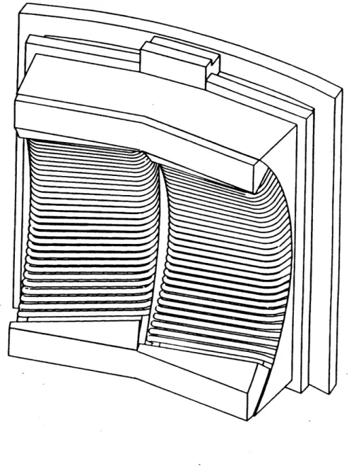
The model of the antenna was composed of one horizontal section of the antenna. The model included the Faraday shield, protection tile, side wall, back plate, and septum (fig. 5.1). It was not necessary to model the current strap since it can be treated separately from the rest of the antenna structure.

Since the major areas of concern were the temperatures of the Faraday shield and protection tiles, a reasonably fine mesh of these elements was created. The mesh was reduced for the side wall and back plate as the temperature gradient decreases in these areas.

The temperature on the base of the back plate is held constant at room temperature (27"C) since the back plate is effectively cooled. The input temperature is also fixed for the cooling fluid (27' for water and -150' for nitrogen gas). Radiation is allowed from the faraday shield and protection tile as noted in figure 5.1 to a wall at room temperature. All other nodes of the model are free to change in temperature.

2. ANSYS® _{is a is a registered trademark of Swanson Analysis} Systems, Inc.

Radiation Elements T=27*C nm.-4 - . m r v Faraday Shield T=27'C Septum Coolant Channel 27'C L1 T=27"C

RF Antenna Finite Element Model

uaua r~au~

The septum, Faraday shield, side wall, and back plate are manufactured from Inconel 625 and are plated with a .001" layer of copper. The protection tile is made of a molybdenum alloy (TZM). The tile and shield also have a titanium carbide (TiC) coating of .0005" depth. The properties (and equivalent properties) used in the rf antenna analysis are summarized in Appendix A.

5.1 Loading

The rf antenna loading constitutes a transient thermal analysis. It consists of a thermal pulse of a certain length of time followed by a cool-down period. During the pulse, the antenna produces electromagnetic waves which heat the plasma as described in section 4.1 . In the course of heating the plasma, the antenna itself is also heated. The resistive rf losses and heat fluxes from the plasma will combine to heat the antenna assembly. One of the functions of the protection tile is to protect the Faraday shield from the plasma heat flux which will cause the tile to rise in temperature.

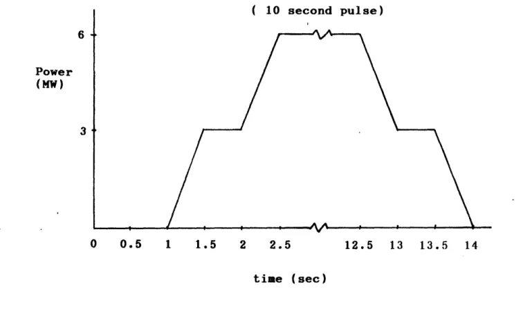
The magnitude of the heat fluxes caused by the plasma and electromagnetic waves was estimated based on the input power and knowledge of the plasma. The input power can be represented as a ramped graph (fig. 5.2) where the maximum power is 6 MW. The length of the pulse is defined in this report as the length of time that the pulse acts at this 6 MW level and is 10 seconds unless otherwise stated. It is assumed that 30% of the input power is uniformly radiated.

6 Power (MW) 3 0 0.5 1 1.5 2 2.5 12.5 13 13.5 14 time (sec)

Figure 5.2 Pulse Input Power

The heat loading on the antenna is shown in figure 5.3 . The Faraday shield has a constant face load of 30 W/cm2 and 25 W/cm2 on each side. The face load is produced by direct radiation from the plasma. The side load is a result of eddy currents induced by the magnetic wave as it passes by and through the Faraday shield. The eddy currents dissipate from the point on the shield where the rf magnetic field intersects the shield.

Since the side loads must be applied to the model at the exterior nodes, the two loads combine on the antenna along a line in a two-dimensional model. In a three-dimensional model,

a more accurate loading distribution is possible since the flux can be evenly distributed on the proper face of the shield.

25

W/c

I

I

I

dOs

7

Figure 5.3 Antenna Loading

The protection tile experiences a parallel heat flux of 1 kW/cma at the leading edge. The flux then decays exponentially. The flux is integrated over the element to determine the flux per element:

(5.1)

S= W er/Adr =--1000JL(e-z/ 1 -e- 1 /A)

where A is a constant which can be scaled from experiments and is set to 1=.002 meters for this analysis.

37

i Bm

1 1

5.2 Two-Dimensional Modelling Strategy

Two-dimensional finite element models offer several important advantages over the three-dimensional alternative. They are usually easier to build since only two dimensions must be considered. This typically results in much fewer elements being needed to construct the model. Fewer elements result in shorter run times. Since three-dimensional elements have more degrees of freedom, the analysis time is longer for each element as compared to the equivalent two-dimensional element which further

increases the overall running time. The additional degrees of freedom, which require a larger stiffness matrix for the solution, also require more memory space to store and solve the intermediate calculations. Thus for simpler, faster, and memory efficient runs, two-dimensional models are greatly preferred. Two-dimensional models should also give identical results to three-dimensional models, assuming that the case is a purely two-dimensional problem.

For the rf antenna model, it was necessary to simulate 8 hours of continuous operation, with a pulse every 20 minutes. In order to obtain reasonable results, a relatively fine mesh was

required resulting in a large model. These considerations made it apparent that a two-dimensional model was desirable. In fact, it was probable that a three-dimensional model would not be able to meet system memory and time limitations.

Unfortunately the rf heating of plasma using cooled tubular heating rods is inherently a three-dimensional problem. The heat enters the rod and is conducted through the tube to the cooled base. In addition, heat is convected to the coolant and carried out of the rod. However, heat is also conducted in the tube around the cooling fluid and then conducted or convected

out the other side. It is this heat flow which causes difficulties in the two-dimensional model.

In order to simulate the circumferential heat flow in the two-dimensional model, the heat flow input parameters were adjusted so that the two-dimensional 'block' would give the same results as a tube. This was done in such a way that the model could be visualized as a three-dimensional problem with an 'equivalent depth' used instead of the actual depth. As a result, the model appeared as an exact cross-section of the real model, with the

same dimensions as the actual antenna (fig. 5.4).

t r. Three-Dimensional Model deq Two-Dimension Figure 5.4

Sr

5.3 Faraday Shield Parameters

The Faraday shield parameters were derived in a general manner. Thus they may be used to convert any three-dimensional tube heat flow problem to two dimensions. Most of the equations were derived from two-dimensional radial heat flow models. The resulting parameters also produced accurate results, however, for loading which was not purely radial.

5.3.1 Cooling Rate

In order to match the cooling rate of the two-dimensional model to that of the actual heating tube, an equivalent depth deq was defined. The cooling rate is

dT

P dT (5.2)

where q is the heat flow, p is the material density, V is the volume, and cp is the specific heat.

In order to maintain the same cooling rate (dT/dt) as well as the same material constants (p and c), the volume of the model is made to equal that of the tube.

V

d = V-cy

(5.3)

21 (ro-r) d, - x (r2-r2) 1

(5.4)

d=

'g (ro+rx

(5.5)

(ro and r_i are the tube outer and inner radii respectively; 1 is the element length.)

The two-dimensional model of the tube is now considered to be a 'block' with a depth into the page of deq. This depth will be maintained for all subsequent calculations.

5.3.2 Conduction

Radial conduction through a hollow cylinder is

q 2lk(T-TI) _(5.6)

In (r/rt)

where k is the material conductivity and To and Ti are the

temperatures at the outer and inner surfaces respectively.

The conduction through a block is

T-T

q = kA

-

(5.7)

ro-ri

where A=deq l.

For the same heat flow (q=qr) the model should have the same temperatures at the boundaries (r0 and ri). The area has been

defined by the geometry and dq . As a result, it is necessary to modify the conduction constant (k). This k will be called the 'equivalent k' and is defined as

k 2(ro

)k

*d. d in (r./ry)

When running a model with keq and purely radial conduction the temperatures at the boundaries will be exact as compared to

theory. The internal temperature profile will not be correct, however, as the profile will be linear instead of curved

(fig. 5.5).

I I I

1T.1

*

Ti

4

t4 t

t

4-Figure 5.5 Temperature Profile Comparison

5.3.3 Convection

The convection coefficient is treated in a similar manner to the

conduction coefficient. Equating the heat flow through the

cylinder to the heat flow through the block gives

q- hA A(T-T.) = hAs(T-TM)

(5.9)

-rh

Sb3

xrb

ANSYS treats the two-dimensional case as having unit depth. In

convection, this is usually taken care of by the input area. The 'area' is then the linear distance along the edge where convection occurs. However, since it is more desirable to think

of the problem in terms of an equivalent depth, an 'actual' area is entered and the unit depth is accounted for by dividing the convection coefficient by deq. Since the convection is calculated by ANSYS as q=hA(T-T,), the results are identical. Thus

h• -rh

h, h (5.11)

A,

s d.,r

(5.12)

5.3.4 Faraday Shield Transverse Heat Flow

If the heat loading on the tube were radial and constant around the circumference of the tube, then the model would not need any side elements. The heat flow would be symmetric and there would be no net heat flow from one side of the tube to the other. This is the ideal case as modelled. For the rf antenna, however, the loading is not symmetric. It is, therefore, necessary to allow conduction between the sides of the tube. The properties of these side panels will not be the same as the other tube elements since they do not figure in the keq

calculation. It is also not possible to derive a simple formula for their properties since the side elements are made necessary due to the presence of a two-dimensional heat flow (as opposed to the one-dimensional radial heat flow created by symmetric loading).

Since the properties were to be applied to the two-dimensional

t

t

V-i, 1

Figure 5.6 Tube Wall Parameters

Then the heat flux through the end wall is

(5.13)

T -T

= k TT

Similarly, the flux through the tube wall in the equivalent model is

=

k,

t

Dividing equation 5.13 by equation 5.14, gives

(5.15)

kw

=

t,(T(-T )

ke

q

t (T,-T3)

In order to approximate the heat fluxes through the tube (q,' and qe'), a tube cross-section model was built (fig. 5.7). Heat

x TEMP SC SMN =400 SMX =551.284 Figure 5.7 1 A =408.405 B =425.214 C =442.023 D =458.833 E =475.642

'emperature Distribution in Tube Model

.4-=492.452

=509.261

=526.07

convection to a fluid was included and a single heat flux was imposed on the model. The solution of the model provided the temperatures and heat flows for equation 5.15. The result was

k, = .

_k

_.

The tube walls were required to allow heat conduction between the two sides of the tube. They should not, however, have any influence in the cooling rate of the tube. Thus, to remove the heat capacity of the tube wall, the specific heat of the walls is set equal to zero (cp=0).

5.4 Fluid Flow Elements

ANSYS contains an element which simulates the heat conduction in a flowing fluid. The equivalent depth should be used in calculating the parameters for this element. Thus

Hydraulic Diameter

Dh

= 4A/P

rZd

Weight Flow

in which i is the mass flow and g is gravity.

46

5.5 Faraday Shield Support Parameters

It is necessary to modify the conduction constant for the Faraday shield supports (septum and side wall) where the tube is inserted. The conduction constant is also modified where the fluid flows directly through the supports. As was done for the tube, an equivalent depth is defined in order to equate the volumes of the two and three-dimensional models:

(w-2r) d. - dw-xrZ

(5.18)

.do . dw-cra

w-2r

The conduction coefficient is then evaluated using the most appropriate and available shape factor (fig. 5.8) [Rohsenow, p.3-121]. The shape factor assumes that both sides of the support are at the same temperature which is reasonable for the rf antenna supports since the differential from one edge to the other should not be large.

1

Figure 5.8 Shape Factor Model

With the shape factor, the heat flow is

q = Fk(TS-Tr) _(5.19)

where

F 2l (5.20)2

In (sinh(

The equivalent conductivity is evaluated by equating the heat flow equations:

q= kA (dT)

_kA

_{= keg (2}

_dec1)

_t

_{Fk ( a-T)}

dxt

(5.21)

Fkt

.: k

_{d e}

These equations are general for a block with a cylindrical hole through it. When the equation is applied to the same block with holes of different diameters, the k 's will have different values. _{Thus the support has three different values for the} conductivity constant, even though it is all made of the same material. _{The back plate maintains the real value of k, while} the side wall and septum k's are modified for the section which houses the tube and for the section which is drilled directly.

5.6 Solid Rod Properties

The cooling of the rf antenna was analyzed for the case where no active cooling was used. _{All cooling would be accomplished} through radiation and conduction to the cooled base. For this case, it was not possible to use the equivalent k as defined for the tube since the value of keq approaches infinity as the internal radius is reduced:

lim

k(ro-r)

_(5.22)

** (5.22)

rlI0

_d

_{q1n (ro/ry)}

Fortunately the tube diameter is small compared to the size of the antenna assembly. _{Therefore, it was reasonable to assume} that the temperature distribution in the cylindrical rod would not vary significantly from an equivalent rod with a rectangular cross-section. As always the equivalent rod must have the same volume as the actual heating rod.

Vcyl~

Vbloc

z 21 - hdql _(5.23)

h

The conduction constant (k) is taken as the real value for the material and of course convection considerations are not relevant for this case.

5.7 Radiation

The heat transfer between surfaces due to radiation can be expressed as

qad - FAoae (T'-T7,)

(5.24)

In this equation, E is the emissivity, a is the Stefan-Boltzmann

constant (a=5.67 x 10

_{WK /m}

_),

_{F is}

_{a form factor and Tsur is}

_the

temperature of the surroundings. In order to maintain the same temperature 'difference' (i.e. to the fourth power), heat flow, and physical constants (a and E) for the tube and equivalent model, the form factor is modified. By comparing the areas of

the two cases, the required form factor is evaluated.

FA = A,

F(21d ) = 2roZl _(5.25)

As for the convection coefficient, it is necessary to divide the form factor by deq in order to account for the unit depth analysis. Thus

d'I

4dg (5.26)

A

=

Id

5.8 Heat Loading

The applied heat loading data is input into ANSYS as heat per unit depth. _{Following the consistent procedure of using the} equivalent depth, the heat flux is

-_=L

For sections such as the protection tile, which do not require an equivalent depth, the heat loading is simply

(5.28)

d

d

6. Material Properties

6.1 Convection Heat Transfer Coefficient

The convection heat transfer coefficient (film coefficient) must be estimated for the cooling fluids. Established empirical correlations for the Nusselt number (Nu) can be used for this

approximation.

6.1.1 Laminar Flow

For fully developed laminar flow in a circular tube with uniform surface heat flux, the Nusselt number is a constant, whereby

Ku 3a

-=

4.36

k

of

=

If the tube has a constant surface temperature, then

Nu

3.66

The loading on the rf antenna did not match either case since the flux is not symmetrical. Since the loading was a flux, however, it was most likely that equation 6.2 would provide the most accurate results. Thus the value of 4.36 was used for the evaluation of the convection heat transfer coefficient.

(6.1)

6.1.2 Turbulent Flow

The Nusselt number for fully developed turbulent flow in circular tubes is a function of the Reynold's number (Re) and Prandtl number (Pr). The Dittus-Boelter equation was used for the rf antenna coolant flow:

Nu = 0.023 Reaa Pr-'

p

uD

ReD p _(6.3)

k

where u3 is the mean velocity of the fluid, D is the tube

diameter while k, cp and p are properties of the fluid.

6.2 Model Properties

Three cooling methods were investigated for the rf antenna; namely liquid water, nitrogen gas, and no active cooling. The three options included radiation cooling to the surrounding walls. Both turbulent and laminar flows were considered for the

fluids.

The fluid flows were assumed to be fully developed. The flow will be fully developed if x/D > 10. With the tube inner diameter being 4 millimeters, an entrance length of only 4 centimeters is required. Thus the fully developed requirement

is fulfilled.

The flow will be laminar for Re < 2300. To be safely in this range, a value of Re = 1000 was chosen. The Reynolds number is fixed to the fluid in ANSYS by means of its mass flow since

Zh = (6.4)

4ReD

The mass flow is converted to a weight flow for the fluid pipe elements as discussed above.

A turbulent flow exists if Re > 4000. A value of Re = 5000 was

used in the antenna analysis.

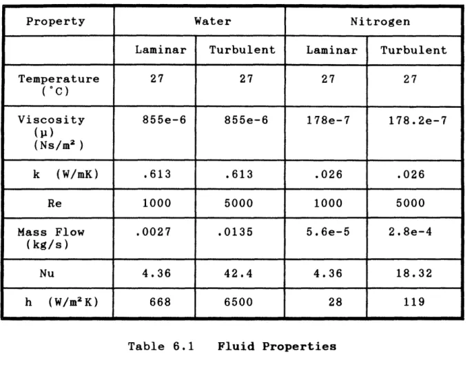
Some of the properties of the fluid should be chosen at the film temperature which is the mean temperature between the wall and fluid mean temperature. Other properties should be at the mean fluid temperature. Since the analysis of the rf antenna is a transient analysis the fluid and wall temperatures are continuously changing. Therefore, it is difficult to choose an appropriate reference temperature. As a result, the initial temperature of the system (room temperature = 27'C) was used as the reference temperature for all properties.

Table 6.1 Fluid Properties

The Reynold's number is directly proportional to the fluid mean velocity (v):

v= RLp

pD

(6.5)

The velocity evaluated from this equation is used to calculate the mass flow. For high Reynold numbers, a high velocity results. For the turbulent nitrogen (Re=5000), v = 18.3 m/s; while the mean velocity for turbulent water is 1.1 m/s. These values are accurate for smooth pipes at room temperature. The

55

Property Water Nitrogen

Laminar Turbulent Laminar Turbulent

Temperature 27 27 27 27

(

c)

Viscosity 855e-6 855e-6 178e-7 178.2e-7

(P)

(Ns/m2 )

k (W/mK) .613 .613 .026 .026

Re 1000 5000 1000 5000

Mass Flow .0027 .0135 5.6e-5 2.8e-4

(kg/s)

Nu 4.36 42.4 4.36 18.32

required velocity will increase as the fluid temperature increases (e.g. v = 32.5 m/s at 200'C; an increase of 75%). The velocity values should be within range of any pump chosen; however, it may still be desired to install disturbances in the pipe flow to 'trip' the fluid into a turbulent state since turbulent flow has a better heat transfer capacity.

7. Results

The rf antenna thermal response was tested using three different cooling methods; liquid water, nitrogen gas, and no active cooling. Radiation cooling was modelled for all three cases. Specific variations were also considered as necessary to fully understand the cooling behavior.

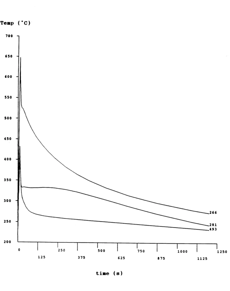
The cooling effectiveness was determined by examining the temperature distribution through the antenna at the maximum temperature and following the cooling period as required. In addition the transient thermal response of three representative nodes was plotted. The location of the nodes is shown in figure 7.1 .

266 281

493

296 299

Figure 7.1 Representative Nodes

Node 281 is located in the middle of the Faraday shield. This provides a good indication of the average temperature along the tube. Nodes 296 and 299 are at the right corner of the tube.

The corner node experiences the maximum temperatures of the tube since it is under the maximum flux (both face and side loads exist here). For the case where no active cooling is provided, the highest temperature will be on the opposite end (the septum side) and is represented by node 266. Node 493 is located on the face of the protection tile where the maximum temperature of the tile exists.

The antenna tube is made from Inconel which has a melting point of T*=1300"C. The copper plating is the limiting factor, there-fore, since it has a melting point of 1085'C. The molybdenum shield has a melting temperature of 2621"C. The safety factor

(n) is defined as

T

-To

n

T

(7.1)

T -To

where To is the initial temperature. Defining the safety factor as a difference of two temperatures removes the dependence on the temperature scale being used. The design is considered safe if n > 1.5. This results in a maximum allowed temperature of 740' on the Faraday shield.

7.1 No Active Cooling

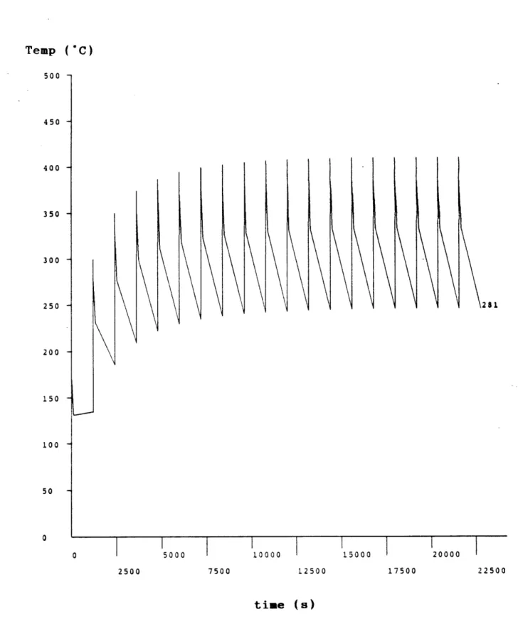
The model for the rf antenna with radiation but no active cooling was constructed to simulate an eight hour day with three

pulses per hour. Each pulse was of ten seconds duration and occurred at equal intervals of twenty minutes. Available system memory, however, limited the run to twenty-one pulses over a six

hour time period. The transient plots for the critical nodes

7500 12500

tine (s)

Figure _7.2

Temperature Response at Node 281 - No Active Cooling 59 Temp ('C) 500 450 400 350 300 250 200 150 100 50 0 ,281 2500 17500 22500 ""' ---""

10000

7500 12500

time (s)

Figure 7.3 Temperature Response at Node 266 - No Active Cooling

60 Temp ( *C) 800 720 640 560 480 400 320 240 160 30 0 5000 2500 15000 20000 17500

Temp ( C)

5000 10000

2500 7500 12500 17500

time (s)

Temperature Response at Node 493 - No Active Cooling

500 450 400 350 300 250 200 150 100 50 0 \493 22500 --- •VVV• Figure 7.4

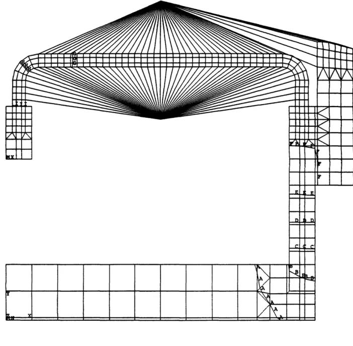
By saving only the temperatures following the final pulse, it was possible to run the model for the full eight hour day. Using these temperatures as the initial conditions in a sub-sequent run allowed full results for the final pulse. The antenna will reach its maximum temperature immediately following the pulse and this distribution is shown in figure 7.5. The maximum temperature of 650"C is located in the left corner of the figure on the Faraday shield under the maximum loading. This results in a safety factor of 1.7 . The maximum temper-ature on the protective tile of 475" is approximately 175' less than that on the shield and the safety factor is 5.8 .

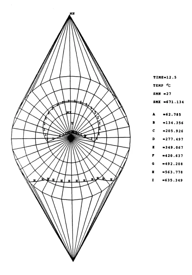
In order to examine the actual temperature profile in the Faraday shield, a rod cross-sectional model was built. The initial temperature of the rod was set to 300'C which was the maximum temperature of the shield before the final pulse. A full ten second pulse was then run. The temperature distri-bution is shown in figure 7.6 and the maximum temperature is 671'C (n=1.64). The maximum temperature occurs in the core of the rod as opposed to the edge where it occurs for the two dimensional model. This is due to the more accurate loading on the rod cross-sectional model which combines in the central

region of the rod. The higher temperature may be caused by the inability of the heat to escape since there is no conduction allowed out of the tube. In the full model, the heat can conduct along the Faraday shield to the cooled back plate. Since the pulse only lasts for ten seconds, however, the conduction should not be significant over this interval. The 20" difference between the two models does not then seem unreasonable.

The transient temperature plots for the three nodes during the final pulse is shown in figure 7.7. The final temperature following the pulse is very close to the initial temperature