HAL Id: hal-02444067
https://hal.archives-ouvertes.fr/hal-02444067
Submitted on 17 Jan 2020HAL is a multi-disciplinary open access archive for the deposit and dissemination of sci-entific research documents, whether they are pub-lished or not. The documents may come from teaching and research institutions in France or abroad, or from public or private research centers.
L’archive ouverte pluridisciplinaire HAL, est destinée au dépôt et à la diffusion de documents scientifiques de niveau recherche, publiés ou non, émanant des établissements d’enseignement et de recherche français ou étrangers, des laboratoires publics ou privés.
4D electrical resistivity tomography (ERT) for aquifer
thermal energy storage monitoring
N. Lesparre, Tanguy Robert, Frederic Nguyen, Alistair Boyle, Thomas
Hermans
To cite this version:
N. Lesparre, Tanguy Robert, Frederic Nguyen, Alistair Boyle, Thomas Hermans. 4D electrical resis-tivity tomography (ERT) for aquifer thermal energy storage monitoring. Geothermics, Elsevier, 2019, 77, pp.368-382. �10.1016/j.geothermics.2018.10.011�. �hal-02444067�
4D electrical resistivity tomography (ERT) for aquifer
1
thermal energy storage monitoring
2
Lesparre Nolwenn1,2, Robert Tanguy3,4,5, Nguyen Frédéric1, Boyle Alistair6, Hermans Thomas1,4,7 3
1 Urban and Environmental Engineering, Applied Geophysics, Liege University, Quartier Polytech
4
1, Building B52/3, Allée de la découverte, 9, B-4000 Liege, Belgium, lesparre@unistra.fr, 5
f.nguyen@uliege.be 6
2 now at: Laboratoire d’Hydrologie et Géochimie de Strasbourg, University of
7
Strasbourg/EOST/ENGEES, CNRS UMR 7517, 1 Rue Blessig, 67084 Strasbourg, France 8
3 previously at: R&D Department, AQUALE SPRL, Rue Montellier 22, B-5380 Noville-les-Bois,
9
Belgium 10
4 F.R.S.-FNRS (Fonds de la Recherche Scientifique), Rue d’Egmont, 5, B-1000 Brussels, Belgium
11
5 Urban and Environmental Engineering, Hydrogeology & Environmental Geology, Liege University,
12
Quartier Polytech 1, Building B52/3, Allée de la découverte, 9, B-4000 Liege, 13
tanguy.robert@uliege.be 14
6 School of Electrical Engineering and Computer Science, University of Ottawa, 800 King Edward
15
Avenue, Ottawa, Ontario, K1N 6N5, Canada, aboyle2@uottawa.ca 16
7 Ghent University, Department of Geology, Krijgslaan 281, 9000 Ghent, Belgium,
17
Thomas.Hermans@ugent.be 18
Abstract
19In the context of aquifer thermal energy storage, we conducted a hydrogeophysical experiment 20
emulating the functioning of a groundwater heat pump for heat storage into an aquifer. This 21
experiment allowed the assessment of surface electrical resistivity tomography (ERT) ability to 22
monitor the 3D development over time of the aquifer thermally affected zone. The resistivity images 23
were converted into temperature. The images reliability was evaluated using synthetic tests and the 24
temperature estimates were compared to direct temperature measurements. Results showed the 25
capacity of surface ERT to characterize the thermal plume and to reveal the spatial variability of the 26
aquifer hydraulic properties, not captured from borehole measurements. A simulation of the 27
experiment was also performed using a groundwater flow and heat transport model calibrated with a 28
larger set-up. Comparisons of the simulation with measurements highlighted the presence of smaller 29
heterogeneities that strongly influenced the groundwater flow and heat transport. 30
Keywords: aquifer thermal energy storage, thermally affected zone, monitoring, electrical resistivity 32
tomography, time-lapse, inversion 33
1 Introduction
34The reduction of fossil fuel consumption is an objective for preserving non-renewable energy 35
resources and reducing the impact of global warming. In this context, renewable and sustainable 36
energies are promoted, e.g. Energy Efficiency Directive 2012/27/EU (European Council, 2012). 37
Smart systems that use heat pumps to transfer heat to or from the ground can take advantage of the 38
thermal stability of the subsurface to reduce energy consumption (Lo Russo et al., 2009; Vanhoudt et 39
al., 2011; Sarbu and Sebarchievici, 2014). Beyond the different existing systems, ground source heat 40
pumps present an inherent thermal resistance with boreholes, while groundwater heat pumps (GWHP) 41
directly use groundwater that presents a relatively stable temperature over seasons. GWHP provide 42
space heating or cooling, domestic hot water production, and are even used to store thermal energy, 43
depending on the season and/or on the specific needs of the infrastructure (Allen and Milenic, 2003; 44
Lo Russo and Civita, 2009). GWHP function through an open loop between two wells or groups of 45
wells drilled in a shallow aquifer. During summer and/or any space cooling periods, water is extracted 46
from the so-called cold well to cool down the infrastructure with the help of heat exchangers (geo-47
cooling). The thermal energy in excess, captured by heat exchangers, is then transferred to 48
groundwater before its re-infiltration into the so-called warm well (Gringarten and Sauty, 1975; 49
Ausseur et al., 1982; Voigt and Haefner, 1987). In winter, the GWHP functions in a reverse mode: 50
water is pumped from the warm well and heat is transferred from groundwater to the building. 51
Groundwater is then re-injected into the cold well with a lower temperature (Ausseur et al., 1982; 52
Ampofo et al., 2006). Theoretically, the heat stored in the aquifer during space cooling periods allows 53
an energy reduction for space heating and inversely with the cold stored during space heating periods 54
for space cooling. Such systems are called aquifer thermal energy storage systems (Sommer et al., 55
2013, 2014; Bridger and Allen, 2014; Possemiers et al., 2015). GWHP working in shallow aquifers 56
requires a relatively small ground surface area by comparison to ground source heat pumps. Thus the 57
thermally affected zone (TAZ) is limited to a volume around boreholes (Sarbu and Sebarchievici, 58
2014). However, the induced temperature variations in the aquifer likely modify the medium 59
properties such as the chemical composition and water quality (Bonte et al., 2013; Jesußek et al., 60
2013). Those changes might in turn impact the system efficiency but also the biodiversity, the 61
microbial activities and consequently the ecosystem functions (Griebler et al., 2016). 62
In addition to controlling the temperature impact often imposed by regulations (Haehnlein et al., 64
2010), the design of GWHP requires a good understanding of the aquifer and heat flow conditions. 65
In particular, issues of thermal short-circuit or recycling between cold and warm wells have to be 66
carefully considered (Banks, 2009; Galgaro and Cultrera, 2013; Milnes and Perrochet, 2013). The 67
propagation of the heat and cold plumes in the aquifer is also highly sensitive to possible variations 68
of hydraulic gradient that could be induced by existing water wells and/or the drilling of additional 69
wells close to the pumping system (Lo Russo et al., 2014) and to the heterogeneity of the subsurface 70
(Bridger and Allen, 2014; Sommer et al., 2013, 2014; Possemiers et al., 2015; Hermans et al., 2018). 71
Methods supplying insights on the heat or cold plume’s propagation in the aquifer have to be 72
developed, notably for delimiting the TAZ, to better anticipate the possible difficulties arising from 73
GWHP implementation. Models of groundwater flow and heat transport are often calibrated with 74
empirical values or from local measurements in boreholes (Lo Russo and Civita, 2009; Liang et al., 75
2011; de Paly et al., 2012; Mattsson et al., 2008; Raymond et al., 2011), ignoring the heterogeneity 76
of the hydrogeological medium. Monitoring the 4D evolution of the TAZ through time is then 77
particularly relevant. The relative proximity of the TAZ to the surface enables a monitoring with non-78
invasive geophysical methods (Hermans et al., 2014). 79
80
Electrical resistivity tomography (ERT) is particularly sensitive to the porous medium temperature 81
(Rein et al., 2004; Revil et al., 1998; Hayley et al. 2007). Moreover, ERT applied in time-lapse (TL) 82
provides spatially distributed information on the changes over time of the porous medium and may 83
target salinity, water content or temperature (for a review on TL ERT see Singha et al., 2015). Thus, 84
TL ERT is specifically appropriate to monitor heat plume development (Hermans et al., 2014). 85
Acquisition systems can work autonomously, allowing the repeated measurements required to 86
achieve sufficient temporal resolution to follow the 3D TAZ development. The method is also 87
minimally invasive and requires low implementation costs compared to a dense network of boreholes. 88
So far, the ability of ERT to monitor heat plumes has been demonstrated in 3D in a laboratory 89
experiment at a scale of a few tens of centimeters (Giordano et al., 2016). Field 2D set-ups confirmed 90
its relevance for monitoring heat storage, tracing experiments and borehole heat exchanger either 91
from surface and/or cross-boreholes measurements (Hermans et al., 2012; Hermans et al., 2015; 92
Giordano et al., 2017; Cultrera et al., 2017). However, 2D interpretation can be limited by out-of-the-93
plane or shadow effects during inversion which can limit the quantitative assessment of temperature 94
(Nimmer et al., 2008). This effect is probably partly responsible for discrepancies observed between 95
ERT-derived temperatures and direct cross-boreholes measurements by Hermans et al. (2015). The 96
use of 3D surveys and subsequent inversion can largely improve imaging of complex 3D subsurface 97
objects (e.g., Van Hoorde et al., 2017). 98
99
In this paper, we image the development of the TAZ during a heat injection and storage experiment 100
using a 3D ERT survey. The accuracy of ERT-derived temperature estimates is explored through 101
synthetic cases that emphasize the method’s sensitivity to target depth and thickness. Results show 102
the ability of surface TL ERT to monitor the 3D development of the TAZ in a shallow aquifer. We 103
compare our results with direct temperature measurements which demonstrates the ability of ERT to 104
supply complementary insights about the sub-surface spatio-temporal dynamic. The ERT-derived 105
temperatures show a general agreement with direct observations, although important discrepancies 106
are observed in the amplitude of the measured variations. The latter are mainly explained by the
107
different representative volumes of the two techniques and the limitations related to the 108
regularized ERT inversion. A groundwater flow and heat transport model calibrated during a
109
previous experimental set-up at a larger scale, is also computed. Its comparison with direct and ERT-110
derived temperature measurements underline the presence of local heterogeneities at the vicinity of 111
the injection well which should be incorporated in the flow and transport model. 112
2 Field experiment
1132.1 Hydrogeological context
114
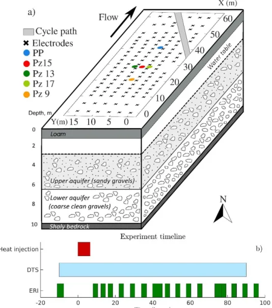
The study site is located on the alluvial plain of the Meuse River at Hermalle-sous-Argenteau, 13 km 115
north-east from Liège, Belgium. From borehole logs analysis, the subsurface medium can be divided 116
into four lithological units. The first layer is composed of loam and presents a thickness of about 1 117
m. Below, the second unit is constituted of sandy loam, gravels and clay to a depth of 3 m. Between 118
3 and 10 m depth, the third layer is composed of gravel and pebbles in a sandy matrix. This third layer 119
hosts the alluvial aquifer. It can be divided in two main units: the upper aquifer, between 3 and 6 m 120
depth, composed of sandy gravels and the lower aquifer, between 6 and 10 m depth, characterized by 121
coarser and cleaner gravels. The water table lies approximately at a depth of 3.2 m. Below 10 m depth, 122
the basement of the aquifer consists of low permeability carboniferous shale and sandstone (Fig. 1). 123
Figure 1: a) Scheme of the experimental set-up and structure of the underground medium (modified 125
from Klepikova et al., 2016). b) The experiment timeline shows the duration of the heat injection and 126
the DTS measurements as well as the moment of ERT acquisitions. 127
128
The site topography is almost flat and the natural hydraulic gradient in the aquifer is approximately 129
0.06% with a north-east direction (Brouyère, 2001). Previous experiments showed that the aquifer is 130
characterized by a high average permeability and by a horizontal and vertical heterogeneity 131
(Dassargues, 1997; Derouane and Dassargues, 1998; Brouyère, 2001). In particular, the upper and 132
the lower parts of the aquifer, ranging respectively in [3-6] m depth and [6-10] m depth present a 133
respective effective porosity of 4% and 8% as estimated from tracer test experiments (Brouyère, 134
2001). Direct measurements of Darcy fluxes were performed to estimate the groundwater flow 135
variations with depth. The lower part of the aquifer present Darcy fluxes in the range of [1-8]x10-3 136
m/s, about one order of magnitude higher than in the upper layer where values range in [1-10]x10-4 137
m/s (Wildemeersch et al., 2014). In a previous multiple tracer tests experiment, the monitoring of the 138
3D spreading of a heat plume resulting from the injection of heated water in the aquifer also showed 139
lateral variations of the medium hydraulic properties (Klepikova et al., 2016), strengthened by 2D 140
cross-borehole ERT and DTS measurements (Hermans et al., 2015). They confirmed the higher flow 141
in the lower part of the aquifer and the lateral heterogeneity of the aquifer that presents zones of 142
preferential flow (Hermans et al., 2015). Similarly, the thermal properties of the aquifer vary with 143
depth as assessed during the ThermoMap project (Bertermann et al., 2013). The thermal conductivity 144
was estimated at 1.37 and 1.86 W/mK and the volumetric heat capacity at 2.22 and 2.34 MJ/m³K in 145
the layers located respectively at depths between 3 to 6 m and 6 to 10 m. 146
2.2 Heating and injection procedure
147
Water was pumped from the aquifer at the pumping well PP (Fig. 1a), its initial temperature was 148
13.4°C and the pumping flow rate was fixed to 3 m³/h. The water was then heated using a mobile 149
water flow heater (Swingtec AQUAMOBIL DH6 system) before being re-injected with a flow rate 150
of 3 m³/h. The heated water was injected in the borehole Pz 15 between 4.5 and 5.5 m depth (Fig. 1). 151
Pz 15 is located in between two boreholes (Pz 13 and Pz 17) screened on the whole aquifer depth 152
allowing DTS measurements (Fig. 1). The water was heated to a temperature of 42°C, i.e. with an 153
increase of 28.6°C from the initial aquifer temperature. The hot water injection lasted 6 hours, but at 154
the end of the injection step, water was injected at a temperature of 14.5°C during 20 minutes due to 155
a technical issue with the water heater. Afterward, a heat storage phase lasted 4 days (Fig. 1b). The 156
injected hot water volume is about 18m³ that can be used to estimate the order of magnitude of the 157
heat plume development. The thermal plume can be assumed to develop in a 3 m height cylinder in 158
the upper part of the aquifer that presents a porosity of 4%. Thus, the thermally affected zone should 159
present a maximum volume of 450 m³ (ignoring conduction effects), developing in a cylinder of about 160
14 m diameter. 161
2.3 3D electrical resistivity data acquisition
162
Electrical resistivity measurements were performed from a grid of electrodes located at the surface to 163
monitor the 3D heat plume evolution in the aquifer. 126 electrodes were placed along 6 profiles of 164
21 electrodes centered on the injection well and parallel to the natural flow direction (Fig. 1a). Along 165
each profile the electrodes spacing was 2.5 m for the 17 central electrodes. Two electrodes at either 166
end of each profile were spaced 5 m apart. That arrangement of electrodes was selected to allow a 167
finer resolution around the injection well together with a greater penetration depth than profiles with 168
equidistant electrodes. Some electrodes located on the northern side of the profiles 1 to 3 could not 169
be hammered into the ground since the field is crossed by a concrete bike path. Thus, 1 or 2 electrodes 170
were missing on those profiles (Fig. 1a). The electrode profiles were separated by 3 m so the electrode 171
grid covers the whole space available to image the plume without degrading the resolution 172
perpendicular to the profiles. Data were acquired with gradient and dipole-dipole protocols along 173
each profile (2D data acquisition). Cross-line measurements were also acquired (Van Hoorde et al., 174
2017), but ignored during inversion due to their low quality. We used an ABEM Terrameter LS 175
connected to a relay switch ES10-64 allowing the acquisition in one shot of the whole data set for the 176
entire electrode grid. A first data acquisition was performed the day before the heated water injection 177
for reconstructing the background image. During the heat storage period 16 acquisitions were 178
performed; once every six hours (Fig. 1b). For the background acquisition, reciprocal measurements 179
were acquired for the whole data set to estimate the measurement error (LaBrecque et al., 1996). 180
Reciprocal measurements correspond to a swap of the electrodes used for current injection and 181
voltage measurements during the “normal” acquisition. A complete normal data set consisted in 3045 182
voltage measurements. For the time-lapse acquisition, the amount of reciprocal data was reduced to 183
1119 to speed up the acquisition. The acquisition delay was set to 0.3 s and the acquisition time was 184
0.5 s. The acquisition duration was 2.5 and 1.5 hours for the background and the time-lapse 185
acquisitions, respectively. 186
2.4 Borehole measurements
187
Single-ended optical fibers were inserted in the Pz13 and Pz17 boreholes located on both side of the 188
injection borehole (Fig. 1a). The optical fibers allow a direct monitoring of the temperature variations 189
in the aquifer during the experiment, performed with an AP Sensing Linear Pro Series N4386. The 190
distributed temperature sensing (DTS) measurements provide a spatial sampling of 0.2 m and a 191
temporal resolution of 2 min. Since the aquifer vertical extension is relatively small (7 m) we choose 192
to preserve the spatial resolution provided by the spatial sampling provided by the DTS. Instead, we 193
preferred reducing the temporal resolution so we applied a running average through time over a 194
20 min window. Two sections of the optical fibers were placed respectively in a chilled and a warm 195
water bath. The cold bath was maintained near 0°C (about 13°C cooler than the aquifer) by regularly 196
adding ice. The baths’ temperature was monitored with Pt100 sensors. The cable ends were placed at 197
the bottom of the boreholes due to the small diameter of boreholes compared to the critical bend 198
radius of optical fibers. Thus the differential attenuation of the light along the single-ended cables 199
could not be estimated (Hausner et al., 2011). Nevertheless, the calibration baths allowed to correct 200
the estimated temperatures, guaranteeing their temporal consistency throughout the experiment. DTS 201
measurements were used for checking the relative temperature change 𝛥𝑇 from the initial state and 202
not for an absolute monitoring of the aquifer temperature. The air temperature increased by 15°C at 203
the end of the experiment. However, this effect is attenuated with depth and, although we can observe 204
a difference at a depth of 1 m in the DTS measurements, no temperature variation below 3 m 205
(saturated zone) is visible. 206
3 Groundwater flow and heat transport model
2073.1 Settings of the hydrogeological model
208
We used the 3D groundwater flow and heat transport model HydroGeoSphere (HGS) (Therrien et al., 209
2010) developed by Klepikova et al. (2016) for the Hermalle-sous-Argenteau experimental site to 210
simulate numerically our experiment and compare temperatures derived from ERT and measured 211
directly with DTS to the simulation. This deterministic model has been constructed and calibrated 212
based on historical data (Dassargues, 1997; Derouane and Dassargues, 1998; Brouyère, 2001) and a 213
multiple tracer experiment, including heat tracer (Wildemeersch et al., 2014; Hermans et al., 2015). 214
215
The model geometry corresponds to the one described by Klepikova et al. (2016), except that we 216
refined the grid around the injection well to accurately model the experiment. In several aspects their 217
experiment differs from the one presented here. They injected the heat tracer at the base of the Pz 9 218
borehole (Fig. 1a), so in the lower unit of the aquifer that is hydraulically more conductive. 219
Furthermore, Pz 9 is screened over the whole thickness of the aquifer (Table 1) allowing heat 220
propagation upward along the borehole. Their experimental design was adapted to constrain the 221
hydraulic conductivity values on the whole aquifer section. In our experiment the temperature 222
changes occurred in the upper part of the aquifer where heat was injected. Therefore, our data were 223
more sensitive to the spatial variability of hydraulic conductivity distribution in the upper area. 224
Moreover, they injected the heated water at a rate of 3 m³/h during 24 hours and 20 minutes, while 225
pumping at a constant discharge rate of 30 m³/h in the pumping well (Fig. 1) in order to speed up the 226
heat propagation in the aquifer. Therefore their experiment supplied information on the hydraulic 227
properties in the whole domain in between the injection borehole Pz 9 and the pumping well (Fig1). 228
In our case, we injected and stored the heat in the Pz 15 borehole so our experiment is more sensitive 229
to hydraulic properties distribution in a smaller region surrounding that borehole. 230
231
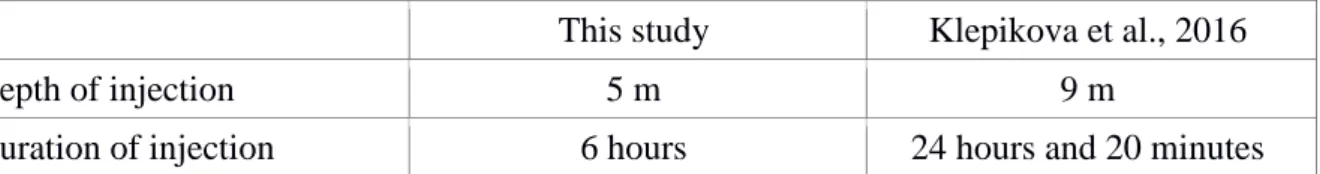
Table 1: Main differences between the experiment of Klepikova et al. (2016) and the one presented 232
in this study. 233
This study Klepikova et al., 2016
Depth of injection 5 m 9 m
Pumping time Only during injection All along the experiment
Pumping rate 3 m³/h 30 m³/h
Injection rate 3 m³/h 3 m³/h
Injection well Pz 15 Pz 9
Injection well screen interval -[5.5 ; 4.5] m -[8.7 ; 3.2] m 234
The inversion process ran by Klepikova et al. (2016) sought the hydraulic conductivity distribution 235
of the Hermalle site aquifer, in between the Pz 9 and the pumping well PP from a monitoring of the 236
temperature changes in the upper and lower part of the aquifer from 11 observation boreholes. They 237
estimated the hydraulic property values with the pilot point method to parametrize the inversion 238
(Fig. 2). Here we use their resulting model to simulate the heat transport in the aquifer with the 239
characteristics of our experiment. The model includes the density effects due to temperature changes 240
(Graf and Therrien, 2005). 241
242
Figure 2: Spatial variability of the hydraulic conductivity K (m/s) models in XY planes for the lower 243
(a) and upper (b) parts of the aquifer obtained from the inversion of transient temperature responses 244
(Klepikova et al., 2016). 245
3.2 Temperature estimates from the HGS model
246
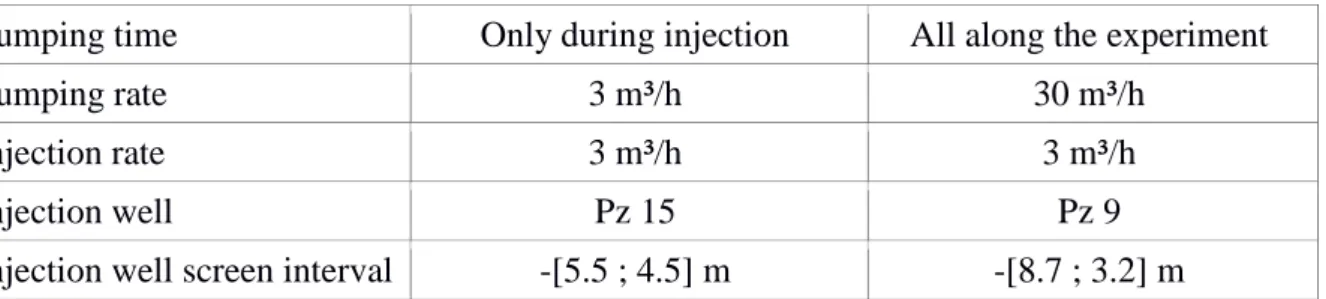
The temperature variations from the HGS model show a TAZ with a half-sphere geometry in the 247
upper part of the aquifer (Fig. 3). In the lower part of the aquifer, the TAZ presents a tail along the X 248
axis (towards NE which is the main flow direction; Fig. 3 c, d). The higher hydraulic conductivity 249
and the greater porosity in the lower part of the aquifer (Fig. 2 a) favors heat propagation with 250
groundwater flow through convection. 8 h after the beginning of the injection, the diameter of the 251
TAZ showing a 𝛥𝑇 of 4°C at a depth of 4.5 m is about 5 m and is slightly more elongated in the X 252
direction. The lower diameter of the model TAZ compared to the above estimate for a cylinder of 253
14 m diameter can be explained by the fact that the model predicts a deeper propagation of the TAZ. 254
Moreover, in the lower part of the aquifer the porosity is set higher in the model than the one used for 255
the cylinder volume evaluation. 47 h after the injection started, the dimension of the model TAZ 256
showing a 𝛥𝑇 of 4°C is slightly reduced to a diameter of about 3 m at a depth of 4.5 m. However at 257
that time, 𝛥𝑇 in the middle of the TAZ is significantly lower, e.g. from 12°C after 8 h (Fig. 3 c) to 258
4°C for the same position after 47h (Fig. 3 d). 259
260
Figure 3: Temperature variation from the initial state estimated by the HydroGeoSphere model, 8 h 261
and 47 h after the injection started on sections in a horizontal layer at -4.5 m (a, b), on cross-262
section at the level of the injection borehole along the electrode profiles (c, d) and perpendicular to 263
the electrode profiles (e, f). The green circles and lines represent the injection and measurement 264
boreholes. The black dotted lines and crosses correspond to the electrodes. 265
4 ERT-derived temperature images reconstruction process
2664.1 Inversion method
267
The image reconstruction process in ERT aims to determine the spatial distribution of bulk resistivity 268
in the medium that best reproduces the resistance measurements. An inverse problem is then solved 269
to iteratively minimize the objective function 𝛹(𝑚): 270 271 𝛹(𝑚) = 𝛹𝑑(𝑑, 𝑚) + 𝜆𝛹𝑚(𝑚), 272 Equation 1 273
where 𝛹𝑑(𝑑, 𝑚) measures the data misfit, 𝛹𝑚(𝑚) defines model constraints for the inversion
274
regularization and 𝜆 is the damping factor that balances the weight of the regularization. We used the 275
EIDORS software for solving the inversion of the ERT data (Polydorides and Lionheart, 2002; Adler 276
et al., 2015). 277
278
The data misfit 𝛹𝑑(𝑑, 𝑚) is evaluated between observed measurements 𝑑 (electrical resistances) and 279
calculated data 𝑓(𝑚) computed from a model of resistivity 𝑚. Model and data are both expressed 280
using their base 10 logarithm. 281
282
For the reconstruction of the medium background, before the introduction of perturbation through 283
heat injection, the absolute values of the medium resistivity are sought and the data misfit is expressed 284 as: 285 𝛹𝑑(𝑑, 𝑚) = ∑ |𝑑𝑖−𝑓𝑖(𝑚)|2 |𝜖𝐵,𝑖| 2 𝑁 𝑖=1 , 286 Equation 2 287
where 𝜖𝐵 are weighting factors accounting for the uncertainty of the measurements. 288
289
For time-lapse inversions, the inversion seeks the variations of resistivity from the background model. 290
The measure of the data misfit is here defined using the difference between the background data 𝑑0𝑖
291
(the subscript 0 refers to the background data) and the monitored data 𝑑𝑖: 292 𝛹𝑑(𝑑, 𝑚) = ∑|(𝑑𝑖− 𝑑0𝑖) − (𝑓𝑖(𝑚) − 𝑓𝑖(𝑚0))|² |𝜖𝑇𝐿,𝑖|² 𝑁 𝑖=1 293
Equation 3 294
where 𝑚0 stands for the model parameter distribution of the background state and 𝜖𝑇𝐿 corresponds
295
to the time-lapse data weighting. 296
297
The insertion of prior information on the medium structure is performed by 𝛹𝑚(𝑚) in the inversion 298
to stabilize the inverse problem: 299
𝛹𝑚 = ||𝑊𝑚(𝑚 − 𝑚0)||2, 300
Equation 4 301
where 𝑊𝑚 represents the regularization matrix that is here the identity matrix (Tikhonov, 1963). The 302
background image 𝑚0 was the result of a first inversion seeking the resistivity values of a medium
303
constituted by four horizontal layers as highlighted by borehole logs analysis and previous ERT 304
experiments (Hermans & Irving, 2017). The four layers correspond to a superficial unit above 1 m 305
depth, below the unsaturated zone extends to 3 m depth, then to a depth of 10 m lies the aquifer over 306
the bedrock. The depth of the interfaces are taken from borehole logs analysis. In the time-lapse 307
reconstruction scheme, 𝑚0 corresponds to the background image that refers to the initial state of the
308
medium. 309
310
The computation of 𝑓(𝑚) is performed using a 3D finite element model built using the Netgen 311
software (Schöberl, 1997). The unstructured mesh is refined close to the electrodes for a better 312
accuracy of the resistance estimation, while elements are coarser further away from the electrodes 313
allowing a reduced computation time. A regular coarse mesh was designed for the inversion in order 314
to reduce the number of model parameters and thus stabilize the inversion procedure. 315
316
The inversion is performed using an iterative Gauss-Newton scheme and at each step a linear search 317
against data misfit seeks the optimum value of the regularization parameter 𝜆that minimizes the 318 weighted residuals 𝜒: 319 𝜒 = √1 𝑁𝛹𝑑(𝑑, 𝑚). 320 Equation 5 321
The inversion is stopped either when the inversion converges, that is when further iteration do not 322
provide a better data fit 𝜒, i.e. no reduction of the objective function 𝛹(𝑚) is observed, or when the 323
desired misfit 𝜒 = |1 − 𝜉| is reached, with 𝜉 = 10⁻². Such a stopping criteria avoids over-fitting data 324
and the presence of artefacts in the resulting image (Kemna, 2000). The data analysis and the method 325
used to determine the error models weighting the data misfit are described in the appendix A.1. 326
4.2 ERT conversion to temperature images
327
Temperature variations in the aquifer induce a change of the medium electrical properties, i.e. the 328
resistivity and its inverse the conductivity. The conductivity variations from the initial state and the 329
temperature changes are related by a linear petrophysical relationship so temperature images can be 330
derived from ERT (Hermans et al., 2014). We consider that bulk conductivity variations in the aquifer 331
are due to changes of the fluid conductivity that depends on fluid salinity and temperature variations. 332
We checked that chemical perturbations produced by temperature changes have a negligible effect 333
on the fluid salinity (Hermans et al., 2015). Thus, the conductivity increase can be quantitatively 334
interpreted in terms of temperature change using the linear relationship: 335 𝜎𝑓,𝑇 𝜎𝑓,25 = 𝑚𝑓(𝑇 − 25) + 1 336 Equation 6 337
where 𝜎𝑓,𝑇 stands for the fluid conductivity at a temperature 𝑇 and 𝑚𝑓 corresponds to the fractional
338
change of the fluid conductivity per degree Celsius around the reference temperature 𝑇 = 25°𝐶. From 339
water samples taken on site the trend between the temperature and the fluid conductivity was 340
estimated to be 𝑚𝑓 = 0.0194 and the fluid conductivity at 𝑇 = 25°𝐶 was evaluated at 𝜎𝑓,25 = 341
0.0791 𝑆 𝑚⁄ (Hermans et al., 2015). 342
343
Temperature change from the initial state 𝛥𝑇 images can be constructed from the observed variations 344
of the bulk conductivity 𝜎𝑏 by converting them with (Hermans et al., 2014; 2015): 345 𝛥𝑇 = 1 𝑚𝑓 (𝜎𝑏,𝑇𝐿 𝜎𝑏,𝐵 𝜎𝑓,𝐵 𝜎𝑓,25 − 1) + 25 − 𝑇𝑖𝑛𝑖𝑡 346 Equation 7 347
𝜎𝑏,𝐵 and 𝜎𝑏,𝑇𝐿 correspond respectively to the bulk conductivity of the background state and of a
time-348
lapse acquisition. 𝜎𝑓,𝐵 = 0.0614 𝑆 𝑚⁄ represents the fluid conductivity at the initial state and was
349
estimated from Eq. (6) with an initial temperature of 𝑇𝑖𝑛𝑖𝑡 = 13.44°𝐶. That initial temperature value 350
corresponds to the average of the temperatures measured along both boreholes using DTS before the 351
heat injection. The estimate of the initial conductivity of the fluid was validated with a value of 𝜎𝑓,𝐵 = 352
0.0598 𝑆 𝑚⁄ by direct measurement with a CTD probe in the injection borehole. 353
4.3 Sensitivity analysis of the ERT-derived temperature images
354
We ran synthetic simulations computed from models of a cylindrical plume with different thicknesses 355
and positions in the aquifer in order to evaluate the sensitivity of the electrode array to the target depth 356
and thickness. The temperature increase in the cylinder was fixed to 17°C and the cylinder diameter 357
to 8 m based on the outcomes of the HGS model. The cylinder was centered on the injection borehole 358
Pz 15 (Fig. 1). The tested cylinder heights varied between 1.5 m and 5 m. The cylinder upper limit 359
positions checked was of -3 m and - 4 m so it is always located below the unsaturated zone (Fig. 4). 360
On all images, we observe that the inversion allows a fairly correct reconstruction of the target shape 361
when the target is located close enough to the electrodes (approximately the distance corresponding 362
to the electrode spacing) or sufficiently thick to be detectable (at least the electrode spacing). We note 363
that the target upper limit is always overestimated by about 2 m and that the amplitude of 𝛥𝑇 364
decreases with depth. The region of higher 𝛥𝑇 in the reconstructed target is also shifted upward the 365
center of the actual target. Moreover, the temperature increase leaks out of the synthetic target 366
delimitation, except in the shallow region where artifacts induce a reduction of the electrical 367
conductivity (Fig. 4). Quantitatively we can compare the estimated temperature increase at the level 368
of the injection borehole Pz15 to the synthetic target as summarized in Table 2. We note that when 369
the target is relatively shallow, that is for an upper limit at -3 m, the increase of the target thickness 370
greatly helps determining more closely the target true temperature. However if the target is only 1 m 371
deeper, the target thickness increase does not allow accurate estimates of the target temperature. 372
373
Table 2: Percentage of the temperature increase estimated by ERT from the synthetic target increase 374
for different cylinder height and upper position. 375 Height \ Upper limit 1.5 m 2.5 m 4 m 5 m -3 m 24 % 44 % 67 % 78 % -4 m 17 % 30 % 41 % 46 % 376
The target blur and the global temperature underestimation are related to the regularization that favors 377
a smooth change from the background model. The smoothing effect hinders a precise location of the 378
target and thus an overestimation of the target depth. Moreover, the estimation of 𝛥𝑇 at depth is 379
degraded by the reduction of the ERT sensitivity with depth (Fig. 4). From those tests, we infer that 380
the geometry of the plume (its size and depth) is fairly estimated, with an overestimation of the plume 381
vertical position when the target depth and thickness correspond to the electrode inter-distances. 382
Furthermore, images underestimate the actual temperature changes in the aquifer. Smoothing effects 383
and the underestimation of the aquifer parameters using TL-ERT are well known and results from the 384
regularization procedure in the inversion (Singha and Moysey, 2006). 385
386
Figure 4: Temperature variation estimates from synthetics built as a vertical cylindrical heat plume. 387
The cylinder thickness is of 1.5 (a, b), 2.5 (c, d), 4 (e, f) and 5 m (g, h) and its upper limit is at -3 m 388
(a, c, e, g) and -4 m (b, d, f, h). The green lines indicate the shape of the cylindrical target, the black 389
crosses correspond to the electrodes. 390
5 Results from field data
3915.1 Background images
392
The 3D inversion of the background ERT data set provides the distribution of the subsurface 393
resistivity with a root mean square of the data misfit of 1.03%. The results are presented by 2D vertical 394
cross-sections corresponding to each acquisition profile (Fig. 5). The images show the vertical 395
variations of the electrical resistivity corresponding to the four lithological units. The superficial 396
conductive layer with a thickness of 1 m and a resistivity of about 115 Ω.m corresponds to the loam 397
unit. Between 1 and 3 m deep the medium presents heterogeneous variations of resistivity with zones 398
of a few meters length showing a resistivity higher than 400 Ω.m and locally values reaching 399
1000 Ω.m while the surrounding medium presents a resistivity of 250 Ω.m. Here the resistive regions 400
might be interpreted by lenses of clean unsaturated gravels in a medium of sandy loam and gravels. 401
Below, in the aquifer layer at a depth between 3 and 10 m the medium presents a median resistivity 402
of 180 Ω.m with some more conductive areas notably below profiles located on Y= 6 and 9 m where 403
the resistivity is around 100 Ω.m. Those conductive anomalies are likely an effect of the pumping 404
well metallic-casing. We note that we do not distinguish any clear resistivity variations related to the 405
different nature of the aquifer upper and lower units. Previous ERT experiments discriminated 406
between the upper and lower regions through a higher resolution cross-borehole survey (Hermans et 407
al., 2015), or through a specific analysis developed for discriminating the different facies of the 408
medium (Hermans and Irving, 2017), which were not used in this study. Finally, the lower layer 409
located below 10 m depth in the bedrock shows a median resistivity of 280 Ω.m. Those values are in 410
accordance with previous ERT investigations on the site (Hermans and Irving, 2017). 411
Figure 5: Electrical resistivity cross-sections extracted below each electrode profile from the 3D 412
model. The black hashed or solid lines represent the injection and measurement boreholes projection. 413
The black crosses correspond to the electrodes. 414
415
5.2 Time-lapse conductivity variation images
416
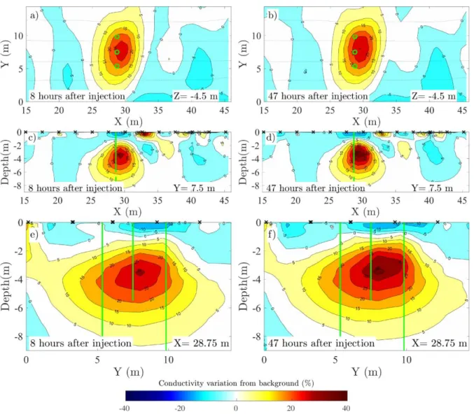
Since conductivity variations vary linearly with temperature we choose to represent that property 417
instead of resistivity variations over selected time steps (8 h and 47 h after the injection started) on 418
sections of the 3D model (Fig. 6). A conductive plume, with a variation between 10 and 30% from 419
the initial state, is observed in the upper part of the aquifer (Fig. 6c to f). The region showing a 420
conductivity increase higher than 10% presents an oval geometry with a horizontal extent of about 421
5 m along the X axis and 10 m in the Y direction (Fig. 6a and b). The plume is not centered on the 422
injection borehole, but is slightly shifted along the X axis, in the same direction as the natural 423
groundwater flow. The region with the highest conductivity change is also slightly shifted in the Y 424
direction. The global shape of the zone affected by conductivity changes does not significantly evolve 425
with time, but the conductivity further increases more than 50 hours after the end of the injection. A 426
second conductive target is observed at Y=0 m, below the first profile which is lacking central 427
electrodes. We interpret this more conductive zone as an artifact related to a lower sensitivity in that 428
region due to the missing electrodes (Fig. 6). The images also present regions with a conductivity 429
decrease from the initial state, mostly in the shallow region but also at depth below profile 1 and at 430
the extremity of the central profiles. In the shallow region, they might be related to changes in the 431
medium saturation above the aquifer. Below, we interpret them as artifacts that are strengthened by 432
our less conservative choice of error model (see Appendix A.1). 433
434
Figure 6: Conductivity variations 8 h and 47 h after the injection started with respect to the 435
background measurements in a horizontal layer at -4.5 m (a, b), on cross-section at the level of the 436
injection borehole along the electrode profiles (c, d) and perpendicular to the electrode profiles (e, f). 437
The green circles and lines represent the injection and measurement boreholes. The black dotted lines 438
and crosses correspond to the electrodes. 439
5.3 ERT-derived temperature images
440
ERT-derived 𝛥𝑇 images show a similar shape and evolution of the TAZ as the conductivity variation 441
images (Fig. 7). On those images, 𝛥𝑇 is fixed to 0°C in regions showing negative contrasts of 442
conductivity since we interpret them as artifacts. The TAZ with a 𝛥𝑇 increase of 4°C from the initial 443
state presents an oval shape in the horizontal plane at Z=-4.5 m with a length of 10 m in the Y 444
direction and a width of 5 m along the X axis (Fig. 7a, b). As on the conductivity variation images, 445
the shift along the X and Y directions of the TAZ with a highest 𝛥𝑇 is observed (Fig. 7c, d, e, f). 446
From the synthetic tests, we deduce that the TAZ oval shape is not an effect of the electrode design 447
or inversion, but reflects the actual shape of the TAZ. This highlights the usefulness of ERT in 448
providing information on the plume anisotropy. ERT-derived 𝛥𝑇 images show a relatively shallow 449
TAZ upper limit, in the region where the method sensitivity is still adequate for detection. However, 450
as observed from the synthetic inversions, the TAZ upper limit deduced from ERT might be 451
overestimated by 2 m. The TAZ should indeed be confined below the water table (3 m depth, Fig. 1). 452
Similarly to the synthetic cases, it is difficult to properly image the shape of the TAZ in the lower 453
part of the aquifer from ERT inversions, due to the low sensitivity (Fig. 4). Quantitatively, 8 hours 454
after the beginning of injection, the derived 𝛥𝑇 reaches locally 12°C in the upper part of the aquifer 455
between the injection borehole and the electrode profile at Y=9 m (Fig. 7). 40 hours later, that region 456
shows a higher 𝛥𝑇 value of 14°C. However, a difference of only 2°C is in the range of uncertainty 457
observed in the synthetic tests, it is thus difficult to confirm this 2°C increase. Nevertheless, we note 458
the persistence of a TAZ on the ERT-derived 𝛥𝑇 images with a similar shape 8 h and 47 h after the 459
injection (Fig. 7). 460
Figure 7: Temperature variation from the initial state estimated from ERT 8 h and 47 h after the 462
injection started in a horizontal layer at -4.5 m (a, b), on cross-section at the level of the injection 463
borehole along the electrode profiles (c, d) and perpendicular to the electrode profiles (e, f). The green 464
circles and lines represent the injection and measurement boreholes. The black dotted lines and 465
crosses correspond to the electrodes. 466
467
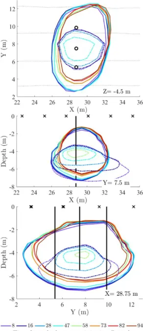
Predictions from the HGS model and ERT-derived 𝛥𝑇 results are represented on cross-sections to 468
ease their comparison (Fig. 8). The edges correspond to the TAZ showing a 𝛥𝑇 of 4°C from the initial 469
state, at different times after the injection. Estimates derived from ERT show a coarser TAZ with a 470
shape preserved all along the experiment, probably due to the smoothing effect of the inversion as 471
demonstrated by the synthetic tests. They illustrate the gradual plume shift along the X and Y 472
directions. Predictions from the HGS model show a smaller TAZ confined at the level of the hot water 473
injection. The dimension of the predicted TAZ shrinks progressively and vanishes after 58 h. 474
Compared to ERT-derived 𝛥𝑇contours, the HGS predictions show also a stronger influence of the 475
natural groundwater flow that transports the plume in the X direction, notably in the lower part of the 476
aquifer. Note that the natural flow was estimated from a regional model (Brouyère, 2001) and has a 477
larger influence in our experiment than in the one used for calibration given the lower pumping rate 478
(Table 1). Finally, the HGS predicted plumes do not show the significant anisotropy with an 479
elongation in the Y direction in the horizontal plane observed on the ERT results. 480
Figure 8: Evolution of the plume shape over time, with a contour line at 𝛥𝑇 = 4°C. The colored lines 481
represent estimates from ERT and the hashed colored lines predictions from the HGS model. Data 482
are presented on cross-sections in a horizontal layer at -4.5 m (a), at the level of the injection borehole 483
along the electrode profiles (b) and perpendicular to the electrode profiles (c). The black circles (a) 484
and lines (b,c) represent the injection and measurement boreholes. The black dotted lines (a) and 485
crosses (b,c) correspond to the electrodes. 486
5.4 Direct temperature measurements
487
DTS direct temperature measurements in the aquifer show that the temperature variation from the 488
initial state 𝛥𝑇 reaches 20°C in the upper part of the aquifer, while in the lower part 𝛥𝑇is about 10°C 489
with a local increase to 15°C (Fig. 9). From the end of the injection, 𝛥𝑇 decreases abruptly at depth 490
below 5 m, while in the upper part 𝛥𝑇 decreases gradually with time. We also note that measurements 491
performed at Y=9.85 m show a larger and stronger print of the TAZ than measurements performed 492
at Y=5.35 m. Thus DTS measurements confirm the plume shift in the Y direction observed from 493
ERT. During the injection, the heat plume propagates at depth until the bottom of the boreholes 494
(Fig. 9). However, the heat increase in depth might be related to local convection around boreholes 495
and not due to heat propagation through the whole aquifer (Hermans et al., 2015; Klepikova et al., 496
2016). 497
Figure 9: Temperature variation from the initial state estimated with the DTS all along the aquifer 498
section at the measurement boreholes Pz17 (a) and Pz13 (b). 499
5.5 Comparison of temperature dynamics
500
The dynamics of 𝛥𝑇 from direct measurements, ERT estimates and the HGS predictions are compared 501
at the level of the measurement and injection boreholes (Pz 13, 15, 17 Fig. 1) at a depth of 4.5 m (Fig. 502
10). That depth corresponds to the highest temperature measured with DTS (Fig. 9). Direct 𝛥𝑇 503
measurements are acquired using DTS data for Pz 13 and Pz 17 and a CTD probe for the injection 504
borehole Pz 15 (Fig. 1). ERT-derived 𝛥𝑇estimates correspond to values extracted from the voxels of 505
the 3D models obtained by the inversion of each data sets acquired after the hot water injection. 506
Similarly, predictions correspond to values extracted from the HGS model voxels at different 507
simulation times. 508
Figure 10: Temperature variations from the initial state at a depth of 4.5 m at the level of Y=5.35 m 510
(a), Y=7.5 m (injection borehole), b) and Y=9.85 m (c). The red zone represents the duration of the 511
heat injection. ERT estimates are obtained from the 3D time-lapse inversions. Model predictions were 512
computed with the HGS model. 513
514
The probe located in the injection well (Y=7.5 m, Fig. 10b) shows an average 𝛥𝑇 value of 27°C 515
during the injection phase. Then 𝛥𝑇 decreases sharply to 0.5°C and softly increases to a peak value 516
of 19°C due to the injection of cold water. 𝛥𝑇decreases then gradually to a value of 7°C at the end of 517
the experiment. Those direct measurements confirm the persistence of the TAZ all along the 518
experiment as observed with ERT (Fig. 7, 8, 10). DTS measurements in neighboring wells do not 519
show the same rebound pattern but instead a faster 𝛥𝑇 decrease at the end of the injection phase. In 520
the measurement borehole at Y=5.35 m, direct 𝛥𝑇measurements reach 20°C during the injection 521
phase and decrease to 3.5°C at the end of the experiment (Fig. 10a). The second measurement 522
borehole at Y=9.85 m shows a different dynamic with a higher 𝛥𝑇 value that reaches 23°C during 523
the injection phase but decreases to a lower value of 0.5°C at the end of the experiment (Fig. 10c). 524
525
ERT-derived 𝛥𝑇 clearly miss to capture the dynamics of the temperature decrease within the TAZ. 526
𝛥𝑇 values are underestimated a few hours after the injection phase and overestimated later (Fig. 10). 527
In general, all 𝛥𝑇 curves derived from ERT are rather stable, although showing a slight decreasing 528
trend, compared to the direct 𝛥𝑇 measurements. In particular ERT–derived 𝛥𝑇 remains higher at the 529
end of the experiment (𝛥𝑇of 6°C and 7.5°C in borehole at Y=5.35 m and Y=9.85 m respectively, Fig. 530
10). Those observations confirm the results of the synthetic tests, showing that the survey design is 531
mostly sensitive to the global temperature change around the well. 532
533
The comparison of the HGS model prediction with the 𝛥𝑇 direct measurements shows that the model 534
globally underestimates 𝛥𝑇 values compared to direct measurements (Fig. 10). The HGS model 535
predicts lower 𝛥𝑇 values at the end of the injection phase in the three boreholes of 12.5°C, 24°C and 536
13.5°C for a Y position of 5.35, 7.5 and 9.85 m respectively (Fig. 10a). At the end of the experiment 537
the HGS model predicts a 𝛥𝑇 value of 1.5°C in the injection borehole, confirming its inability to 538
represent the TAZ persistence. At that time, in both measurement boreholes show similar 𝛥𝑇 values 539
of about 1°C. 540
6 Discussion
541The experiment performed here demonstrates the capacity of ERT to deliver useful information about 542
the 4D evolution of a thermal plume in a shallow aquifer. ERT-derived 𝛥𝑇 images supply information 543
on the plume anisotropy in a horizontal plane and its persistence all along the experiment (Fig. 7, 8, 544
10). The plume anisotropy is attested with synthetic tests but cannot be deduced from direct 545
measurements as boreholes close to the injection well are lacking along the X axis. However, direct 546
measurements in the injection well confirm the TAZ persistence through time (Fig. 10b). So the 547
performed experiment provides an interesting insight on the aquifer storage heat capacity not 548
expected by the HGS model. The revealed anisotropy in the XY direction by ERT might indicate the 549
presence of a preferential water flow path bypassing hydraulic barriers. Such a preferential flow path 550
in the upper part of the aquifer can be related to clay lenses channeling groundwater flow in the Y 551
direction. Despite TL ERT supplying smoothed results due to regularization, the method has the 552
capacity to provide useful insights about local hydraulic conductivity heterogeneity. The suspected 553
local heterogeneities have a strong influence on the groundwater flow and hence on heat transport. 554
However, those small heterogeneities are not taken into account in the existing HGS model. The 555
hydraulic parameters used for the simulation should be adjusted around the injection well to 556
reproduce the plume evolution. Indeed, the hydraulic parameters were determined during a previous 557
experiment representative of a larger scale. The integration of hydraulic parameter variations at that 558
smaller scale into the model could help reproducing the horizontal anisotropy of the TAZ 559
development revealed by ERT. 560
561
In this specific experiment, although ERT identifies the trend, it does not accurately identify
562
the temporal fluctuations of𝛥𝑇. Indeed, DTS measurements show a significant 𝛥𝑇 decrease in both
563
monitored boreholes, while ERT only indicates a slight decreasing trend (Fig. 10). The agreement 564
is better in the injection well. Such examples illustrate the difficulty in comparing data 565
representative of 𝛥𝑇changes in different volumes. On the one hand, heat loss towards the atmosphere 566
might have favored the 𝛥𝑇 decrease observed with DTS within wells. On the other hand, since ERT 567
acquisitions are sensitive to temperature changes in a large volume, their estimates might better reflect 568
the matrix heat storage and release. DTS and CTD measurements are bathed in the borehole water 569
and thus not directly connected to the conditions in the aquifer. In addition, the injection of 570
unwanted cold water further complicated the distribution of temperature in the aquifer,
571
creating an anomaly below the resolution of ERT.
572 573
Quantitatively, the ability of ERT to image the dynamics compared to direct measurements is also 574
limited since we note an underestimation of ERT-derived 𝛥𝑇 values a few hours after the injection 575
phase and an overestimation later. This is a direct consequence of the regularization, as highlighted 576
by the synthetic inversions (Singha and Moysey, 2006). In practice, a small plume with high 577
temperature yields the same image as a large plume with a lower temperature. Combined with
578
the slow dynamic characteristic of a storage experiment, it generates ERT images with limited
579
amplitude variations, but with the correct trend.
580 581
Due to regularization, ERT-derived 𝛥𝑇 images also present a shift in the vertical position of the plume 582
and a coarse shape of the TAZ, both identified with synthetic tests. The effect of blur could be 583
attenuated by reducing the acquisition time, by acquiring a limited amount of reciprocal data (Rucker, 584
2014). Other regularization method such as covariance constraints or minimum-gradient support 585
might help overcome the smoothing effect and improve the delineation of the TAZ (Hermans et al., 586
2016b; Fiandaca et al., 2015; Nguyen et al., 2016). Furthermore, ERT lacks sensitivity in the 587
horizontal dimension due to the electrode inter-distance and the volume integrative sounding of the 588
method. Observed changes with ERT are therefore representative of an average temperature variation 589
in a 3D volume that prevents the reconstruction of an accurate TAZ shape and temperature estimate. 590
The decrease of the ERT sensitivity with depth also hinders delimiting precisely the TAZ in the deeper 591
region. This is further complicated due to the higher groundwater flux easing the plume transport as 592
shown in the HGS model and DTS measurements (Fig. 2, 3, 9). 593
594
Discrepancy with direct measurements, providing local information of the medium properties 595
surrounding the boreholes might be partly explained by perturbations in water circulation related to 596
boreholes drilling and screening. Indeed, we suspect that strong temperature variations observed in 597
the lower part of the aquifer during the hot water injection might be due to internal flow (Fig. 9). The 598
integrative nature of ERT might also affect the comparison with local measurements. The latter, 599
coupled to the adverse effects of inversion also hinders ERT-derived 𝛥𝑇 images to reflect properly 600
the TAZ dynamic. However, beyond the production of ERT-derived 𝛥𝑇 images, discrepancies in the 601
sensitivity of ERT and DTS could be exploited to better constrain hydraulic properties of the aquifer 602
close to the injection borehole, considering they supply complementary insights on the medium 603
properties. The information about the TAZ shape development from ERT can help conceptualizing 604
the spatial variability of hydraulic properties in the aquifer, while direct measurements furnish a 605
quantitative estimate of the temperature variations. So coupled inversion fitting simultaneously the 606
surface resistance measurements and the direct temperature acquisitions is worth considering to 607
evaluate accurately the TAZ location and geometry (Pollock and Cirpka, 2012). The coupled 608
inversion would remove the regularization smoothing and would help refining the hydraulic property 609
distribution around the injection well, which strongly affects predictions. Alternatively, the set-up of 610
a stochastic inversion by model falsification such as a prediction focused approach would also benefit 611
from the complementary nature of ERT and DTS data (Hermans et al., 2016a, 2018). Such a 612
methodology presents the advantage that the developed analysis directly focuses on the prediction of 613
the TAZ with the different measurement types, also avoiding any regularization. 614
7 Conclusion
615Although a quantitative estimation of temperature was not possible in this experiment, due to the 616
inherent limitations of inversion, our study demonstrates the pertinence of the minimally invasive 4D 617
ERT method to provide qualitative, complementary insights on the development of a thermal plume 618
in a shallow aquifer. The ERT-derived 𝛥𝑇 images obtained here inform about the anisotropic shape 619
of the thermal plume and its persistence all along the experiment. Hence, the method indicates the 620
presence of local heterogeneities at the vicinity of the injection well and the aquifer heat storage 621
capacity confirmed by direct measurements. The anisotropic behavior cannot be validated using direct 622
temperature measurements as it would have required a denser network of boreholes close to the 623
injection well (Fig. 1). Thus, ERT measurements provide crucial information for the set-up of 624
groundwater heat pumps (GWHP), which requires an accurate knowledge of the spatial variability of 625
the aquifer’s hydraulic and heat capacity properties. So, the insertion of a correct distribution of the 626
hydraulic properties in the hydrogeological model has to be performed for estimating the likely shape 627
and extension of the TAZ for different GWHP injection regimes. Surface ERT could be used as a 628
control tool for monitoring the successful functioning of GWHP in operation. 629
630
However, the sensitive analysis we performed show that the ERT sensitivity to the plume decreases 631
strongly with the plume depth and depends also on its dimension. Thus, the qualitative 632
characterization of the TAZ performed through ERT inversion is strongly influenced by the TAZ 633
depth. Indeed, the method struggles to provide the shape of the TAZ in the lower part of the aquifer. 634
In our case, most of the TAZ is really shallow, reaching the groundwater table 3 m deep, so the 635
method is sensitive to changes induced in the subsurface by the TAZ development. Nevertheless, for 636
a deeper TAZ, the electrode design should be adapted to explore the medium at greater depths. This 637
can be done by using a larger distance between electrodes but at the cost of a lower spatial resolution. 638
Acknowledgments
639The work by Nolwenn Lesparre was supported by the project SUITE4D from a BEcome a WAlloon 640
REsearcher fellowship fund co-financed by the Department of Research Programs of the Federation 641
Wallonia – Brussels and the COFUND program of the European Union. The field experiments was 642
made possible thanks to the F.R.S.-FNRS research credit 4D Thermography, grant number J.0045.16. 643
We gratefully acknowledge Thomas Kremer and Solomon Ehosioke who participated to the field 644
works and data acquisition supervision. 645
Appendix A.1 Data analysis and error model
646We assume that the data (resistance measurements) are uncertain due to noise and that the latter is 647
composed of a random component and a systematic one correlated over time. The effect of systematic 648
error, including modeling errors, can be canceled out by subtraction when working with data-649
differences inversion (LaBrecque and Yang, 2001). The weighting factors 𝜖𝐵 and 𝜖𝑇𝐿 for the 650
background and time-lapse inversions have to be correctly evaluated. As suggested by Slater et al. 651
(2000) and Lesparre et al. (2017), we use the analysis of normal to reciprocal disparities. First, 652
resistance data were sorted to remove outliers and the data were selected so they presented a repetitive 653
error lower than 1% and a reciprocal error lower than 5% for each time step. The total number of 654
filtered data at each time step was reduced from 3045 to 1948 measurements. 655
656
For the background image, an error model 𝜖𝐵 was fit to the measured difference |𝑅𝑁− 𝑅𝑅| between
657
the normal 𝑅𝑁 and reciprocal resistance 𝑅𝑅 after removing outliers and bining by ⟨𝑅⟩. The error𝜖𝐵 658
varies linearly with resistance (Fig. A.1 a, Slater et al., 2000): 659 𝜖𝐵 = 𝑎𝐵+ 𝑏𝐵⟨𝑅⟩, 660 Equation A.1 661 with 662 ⟨𝑅𝑖⟩ =(𝑅𝑁,𝑖+𝑅𝑅,𝑖)
2 for all 𝑖 where
|𝑅𝑁,𝑖−𝑅𝑅,𝑖|
⟨𝑅𝑖⟩ < 0.05 .
663
Equation A.2 664
For the estimate of an error model of the time lapse inversions, normal and reciprocal data at a given 665
time were compared to the background measurements (Lesparre et al., 2017). The normal difference 666
between times t0 and ti as 𝛥𝑙𝑜𝑔𝑅𝑁 = 𝑙𝑜𝑔𝑅𝑁,𝑖− 𝑙𝑜𝑔𝑅𝑁,0, and the reciprocal difference as 𝛥𝑙𝑜𝑔𝑅𝑅 =
667
𝑙𝑜𝑔𝑅𝑅,𝑖− 𝑙𝑜𝑔𝑅𝑅,0 were used in the time lapse inversions because the data fit were in the logarithmic 668
domain. The difference error model 𝜖𝑇𝐿 was then fit to the measured value of the normal-reciprocal
669
discrepancy |𝛥𝑙𝑜𝑔𝑅𝑁− 𝛥𝑙𝑜𝑔𝑅𝑅| that varies linearly with the inverse of the resistance (Fig. A.1 b, 670 Lesparre et al., 2017): 671 𝜖𝑇𝐿 = 𝑎𝑇𝐿+𝑏𝑇𝐿 ⟨𝑅⟩ 672 Equation A.3 673
Figure A.1: Measured and model error from the normal and reciprocal acquisition for the background 674
(a) and the time-lapse (b) inversions. 675
676
The error model parameters 𝑎𝐵, 𝑏𝐵, 𝑎𝑇𝐿 and 𝑏𝑇𝐿 were estimated by fitting the measured errors as a
677
function of ⟨𝑅⟩ (Fig. A.1). For the time-lapse error estimate, ⟨𝑅⟩ also expresses as stated in Eq. A.2. 678
Error data were divided into classes of ⟨𝑅⟩ with four bins per decade of 𝑅𝑖, logarithmically equally 679
spaced. For each bin the average µ and the standard deviation 𝜎 were estimated (Koestel et al., 2008). 680
The choice of the error threshold on which the error model is fitted impacts the data weighting and 681
so the residuals 𝜒 that are used as a stopping criteria (see Eq. 5). We choose to fit both error models 682
to µ + 𝜎 2⁄ (Fig. A.1) in order to be more sensitive to conductivity variations due to the hot water 683
injection. 684
References
685Adler, A., Boyle, A., Crabb, M.G., Gagnon, H., Grychtol, B., Lesparre, N., Lionheart, W.R., 2015. 686
EIDORS Version 3.8. In Proc. of the 16th Int. Conf. on Biomedical Applications of Electrical 687
Impedance Tomography. 688
Allen, A., Milenic, D., 2003. Low-enthalpy geothermal energy resources from groundwater in 689
fluvioglacial gravels of buried valleys. Appl. Energy 74, 9–19, http://dx.doi.org/10.1016/S0306-690
2619(02)00126-5. 691
Ampofo, F., Maidment, G.G., Missenden, J.F., 2006. Review of groundwater cooling systems in 692
London. Appl. Therm. Eng., 26(17), 2055-2062, 693
http://dx.doi.org/10.1016/j.applthermaleng.2006.02.013. 694
Ausseur, J.Y., Menjoz, A., Sauty, J.P., 1982. Stockage couplé de calories et de frigories en aquifère 695
par doublet de forages. J. Hydrol., 56(3), 175-200, http://dx.doi.org/10.1016/0022-1694(82)90012-9. 696
Banks, D., 2009. Thermogeological assessment of open-loop well-doublet schemes: a review and 697
synthesis of analytical approaches. Hydrogeol. J., 17(5), 1149-1155, 698
http://dx.doi.org/10.1007/s10040-008-0427-6. 699
Bertermann, D., Bialas, C., Rohn, J., 2013. ThermoMap — area mapping of superficial geothermic 700
resources by soil and groundwater data. Available at http://geoweb2.sbg.ac.at/thermomap/. 701
Bonte, M., van Breukelen, B.M., Stuyfzand, P.J., 2013. Temperature-induced impacts on 702
groundwater quality and arsenic mobility in anoxic aquifer sediments used for both drinking water 703
and shallow geothermal energy production. Water Res., 47(14), 5088-5100, 704
http://dx.doi.org/10.1016/j.watres.2013.05.049. 705
Bridger, D.W., Allen, D.M., 2014. Influence of geologic layering on heat transport and storage in an 706
aquifer thermal energy storage system. Hydrogeol. J., 22(1), 233-250, 707
http://dx.doi.org/10.1007/s10040-013-1049-1. 708
Brouyère, S., (Ph.D. thesis), 2001. Etude et modélisation du transport et du piégeage des solutés en 709
milieu souterrain sariablement saturé. University of Liege (unpublished). 710
Cultrera, M., Boaga, J., Di Sipio, E., Dalla Santa, G., De Seta, M., & Galgaro, A., 2017. Modelling 711
an induced thermal plume with data from electrical resistivity tomography and distributed 712
temperature sensing: a case study in northeast Italy, Hydrogeol. J., 1-15. 713
http://dx.doi.org/10.1007/s10040-017-1700-3 714
Caterina, D., Beaujean, J., Robert, T., Nguyen, F., 2013. A comparison study of different image 715
appraisal tools for electrical resistivity tomography. Near Surf. Geophys., 11(6), 639-657, 716
http://dx.doi.org/10.3997/1873-0604.2013022. 717
Dassargues, A., 1997. Modeling baseflow from an alluvial aquifer using hydraulic-conductivity data 718
obtained from a derived relation with apparent electrical resistivity. Hydrogeol. J., 5(3), 97-108, 719
http://dx.doi.org/:10.1007/s100400050125. 720
Derouane, J., Dassargues, A., 1998. Delineation of groundwater protection zones based on tracer tests 721
and transport modeling in alluvial sediments. Environ. Geol., 36(1–2), 27–36, 722
http://dx.doi.org/10.1007/s002540050317. 723
de Paly, M., Hecht-Méndez, J., Beck, M., Blum, P., Zell, A., Bayer, P., 2012. Optimization of energy 724
extraction for closed shallow geothermal systems using linear programming. Geothermics 43, 57–65, 725
http://dx.doi.org/10.1016/j.geothermics.2012.03.001. 726
European Council, 2012. Directive 2012/27/EU of the European Parliament and of the Council of 25 727
October 2012 on energy efficiency, amending Directives 2009/125/EC and 2010/30/EU and repealing 728
Directives 2004/8/EC and 2006/32/EC. Official Journal of the European Union, Legislative acts. 729
Brussels, Belgium. 730