Projected changes to precipitation extremes for northeast
Canadian watersheds using a multi-RCM ensemble
A. Monette,
1L. Sushama,
1M. N. Khaliq,
1,2R. Laprise,
1and R. Roy
1,3,4 Received 1 February 2012; revised 21 May 2012; accepted 22 May 2012; published 4 July 2012.[1]
This study focuses on projected changes to seasonal (May
–October) single- and
multiday (i.e., 1-, 2-, 3-, 5-, 7-, and 10-day) precipitation extremes for 21 Northeast
Canadian watersheds using a multi-Regional Climate Model (RCM) ensemble available
through the North American Regional Climate Change Assessment Program (NARCCAP).
The set of simulations considered in this study includes simulations performed by six
RCMs for the 1980
–2004 period driven by National Centre for Environmental Prediction
reanalysis II and those driven by four Atmosphere-Ocean General Circulation Models
(AOGCMs) for the current 1971
–2000 and future 2041–2070 periods. Regional frequency
analysis approach is used to develop projected changes to selected 10-, 30- and 50-yr return
levels of precipitation extremes. The performance errors due to internal dynamics and
physics of the RCMs and those due to the lateral boundary data from driving AOGCMs are
studied. The use of a multi-RCM ensemble enabled a simple quantification of RCMs
’
structural and AOGCM related uncertainties in terms of the coefficient of variation.
In general, the structural uncertainty appears to be larger than that associated with the
choice of the driving AOGCM for majority of the precipitation characteristics and
watersheds considered. Analyses of ensemble-averaged projected changes to various return
levels show an increase for most of the watersheds, with smaller changes and higher
uncertainties over the southeasternmost watersheds compared to the rest. It is expected that
increases in return levels of precipitation extremes will have important implications for
water resources related activities such as hydropower generation in this region of Canada.
Citation: Monette, A., L. Sushama, M. N. Khaliq, R. Laprise, and R. Roy (2012), Projected changes to precipitation extremes for northeast Canadian watersheds using a multi-RCM ensemble, J. Geophys. Res., 117, D13106, doi:10.1029/2012JD017543.
1.
Introduction
[2] In a warmer projected climate, the water-holding
capacity of the atmosphere, and hence the evapotranspiration and the precipitation potential, is expected to increase and this favors increased climate variability, with more intense pre-cipitation [Trenberth et al., 2003]. Such changes to the inten-sity and frequency of precipitation extremes can in turn lead to enormous environmental, social and political repercussions [Emori and Brown, 2005; Tebaldi et al., 2006]. It, therefore, becomes necessary to assess changes to extremes and associ-ated uncertainties in the context of a changing climate, to support proper management and adaptation strategies.
[3] The primary tools to study anticipated climate changes
are the coupled global and regional nested models and the transient climate-change projections obtained when those models are run with projected anthropogenic forcing [Alley et al., 2007]. Global Climate Models (GCMs), because of their still relatively coarse resolution, have difficulties in simulating extreme weather events with the intensity and frequency comparable to what is observed, particularly pre-cipitation extremes. Regional Climate Models (RCMs), with their higher spatial resolution, compared to that of the GCMs, allow for greater topographic realism and finer-scale atmospheric dynamics to be simulated and thereby better represent extremes as demonstrated in a number of recent studies [Feser, 2006; Seth et al., 2007; Prömmel et al., 2010; De Sales and Xue, 2010; Di Luca et al., 2011]. This improved representation of severe weather phenomena in RCMs has motivated various studies on projected changes to heavy precipitation on the basis of RCM simulations for different parts of the world [Christensen and Christensen, 2003; Fowler et al., 2005; Beniston et al., 2007; May, 2008; Nikulin et al., 2011; Mladjic et al., 2011]. While some of these studies used a single RCM in their analysis, the use of multi-RCM ensembles is highly recommended. multi-RCMs are associ-ated with various sources of uncertainties [de Elía et al., 2008], including (1) structural uncertainty associated with
1
Centre Étude et Simulation du Climat à l’Échelle Régionale, University of Quebec at Montreal, Montreal, Quebec, Canada.
2
Global Institute for Water Security, University of Saskatchewan, Saskatoon, Saskatchewan, Canada.
3Ouranos, Montreal, Quebec, Canada. 4
Hydro-Quebec, Varennes, Quebec, Canada.
Corresponding author: A. Monette, Centre Étude et Simulation du Climat à l’Échelle Régionale, University of Quebec at Montreal, 201 Ave. President-Kennedy, Montreal, Quebec, Canada H3C 3P8.
(dd.031986@gmail.com)
©2012. American Geophysical Union. All Rights Reserved. 0148-0227/12/2012JD017543
model formulation (e.g., domain size and location, nesting and relaxation technique, physical processes and parameter-ization), (2) internal variability (triggered by differences in the initial conditions), and (3) dependence on lateral bound-ary forcing (i.e., choice of GCM). Multi-RCM ensemble as in PRUDENCE [Christensen et al., 2007] and ENSEMBLES [Christensen et al., 2009] projects over Europe is essential to better quantify various uncertainties. The North American Regional Climate Change Assessment Program (NARC-CAP) [Mearns et al., 2009] is such a multi-RCM ensemble project over North America.
[4] This study focuses on the evaluation and assessment of
future changes to selected return levels of seasonal single-and multiday (i.e., 1-, 2-, 3-, 5-, 7- single-and 10-day) precipitation extremes over 21 selected northeast Canadian watersheds spread mainly across the province of Quebec and extending through some parts of Ontario and Newfoundland and Lab-rador provinces, using the NARCCAP multi-RCM ensemble and Regional Frequency Analysis (RFA) approach [Hosking and Wallis, 1997]. These watersheds are very important to hydroelectric power generation and therefore information on projected changes to extreme precipitation is important for better management and planning of reservoirs in the region. In fact, 96% of the total energy produced in the province of Quebec is hydro-based and is thus very important to the economy of the province (Ministère des Ressources natur-elles et de la Faune du Québec, 2009; http://www.mrn.gouv. qc.ca/). In addition, the ‘Plan Nord’ (http://plannord.gouv. qc.ca/) launched recently by the Quebec Government is planning to generate additional hydroelectricity from the same region in the coming years. No similar comprehensive study of extreme precipitation characteristics has been undertaken so far for the region, particularly at the watershed scale. A recent study by Mladjic et al. [2011] looked at projected changes to single- and multiday precipitation extremes, for various climatic zones in Canada, using the RFA approach and an ensemble of Canadian RCM (CRCM) simulations. Their results suggest significant increases in regional return levels for both single- and multiday precipi-tation extremes, for the climatic regions considered in their study. Since the study was based on a single-model ensem-ble, it was possible only to address uncertainty associated with the internal variability of the RCM and natural vari-ability of the driving Atmospheric-Ocean General Circula-tion Model (AOGCM). Following this, Mailhot et al. [2012] analyzed precipitation extremes for the same climatic
regions over Canada considered by Mladjic et al. [2011], but using multi-RCM NARCCAP simulations; their findings agree in general to those of Mladjic et al. [2011].
[5] The paper is organized as follows. A brief description
of the NARCCAP simulations and the observed data used in this study are given in section 2. The methodology used is described in section 3. Section 4 presents results related to the assessment of various errors and uncertainties in the precipitation characteristics considered based on NARCCAP simulations followed by projected changes to these char-acteristics. Discussion and main conclusions of the study are provided in section 5.
2.
Simulations and Observations
2.1. NARCCAP Simulations
[6] The precipitation extremes analyzed in this study are
derived from the multi-RCM ensemble available from NARCCAP. The six RCMs participating in the NARCCAP program are run over similar North American domains covering Canada, USA and most of Mexico; the acronyms and full names of the participating RCMs are given in Table 1. Further details of individual models are available from NARCCAP (www.narccap.ucar.edu/data/rcm-characteristics. html) and Mearns et al. [2009]. It should be noted that all RCMs use roughly the same horizontal resolution of 50 km, but different projections.
[7] The protocol of NARCCAP demands that each
par-ticipating RCM be driven by the National Center for Envi-ronmental Prediction (NCEP) reanalysis and by two distinct AOGCMs for the SRES (Special Report on Emission Sce-narios) A2 scenario [Mearns et al., 2009]. At the time of this study, all six RCMs (CRCM, RCM3, MM5I, ECP2, WRFG and HRM3) had completed simulations driven by both NCEP and at least one AOGCM. The four AOGCMs used to drive the RCMs are CGCM3, CCSM3, HadCM3 and GFDL (see Table 1). Eight RCM-AOGCM pairs were available at the time of the study: two RCMs (CRCM and RCM3) had been driven by two AOGCMs each and the other four RCMs (WRFG, ECP2, MM5I and HRM3) had been driven by only one AOGCM.
[8] The NCEP-driven simulations are available for the
1980–2004 period, while the AOGCM-driven simulations are available for the current 1971–2000 and future 2041–70 peri-ods. The NCEP-driven simulations are used to verify simu-lated precipitation characteristics of individual NARCCAP
Table 1. Names and Acronyms of Six NARCCAP RCMs and Details of AOGCM Driven RCM Simulations Considered in This Study
RCM AOGCM Driven RCM Simulations
Name and Modeling Group Acronym AOGCM Simulation Acronym
Canadian Regional Climate Model (Ouranos) CRCM Canadian Global Climate Model, version 3: CGCM3 CRCM_CGCM3 Community Climate Model, version 3: CCSM CRCM_CCSM
Regional Climate Model 3 RCM3 CGCM3 RCM3_CGCM3
(University of California at Santa Cruz) Geophysical Fluid Dynamics Laboratory Model: GFDL RCM3_GFDL Hadley Regional Model 3 (Hadley Centre) HRM3 Hadley Centre Climate Model, version 3: HadCM3 HRM3_HADCM3 Weather Research and Forecasting Model
(Pacific Northwest National Laboratory)
WRFG CCSM WRFG_CCSM
MM5-PSU/NCAR Mesoscale Model (Iowa state University)
MM5I CCSM MM5I_CCSM
Experimental Climate Prediction Centre Regional Model (University of California at San Diego)
RCMs, while the AOGCM-driven current and future simula-tions are used in the assessment of projected changes to stud-ied precipitation characteristics, as discussed in detail in the section on methodology. Throughout this article, the dif-ferent NARCCAP RCM simulations will be referred to as ‘RCM_LBC’, where RCM stands for the acronym of the respective RCM and LBC for the lateral boundary condition, i.e., NCEP or the AOGCM driving the regional model at its boundaries. For example, CRCM simulation driven by CGCM3 will be referred to as CRCM_CGCM3.
[9] Though the simulation domains of the RCMs cover
most of North America, this study focuses on the northeast part of the domain, which consists of 21 watersheds located mainly in the Quebec province of Canada. The watersheds are shown in Figure 1 and further details are given in Table 2. 2.2. Observed Data
[10] The observed precipitation extremes used in this
study are derived from a gridded daily precipitation data set at 10-km resolution developed by Hydro-Quebec [Jeannée and Tapsoba, 2010], for the province of Quebec and parts of the adjoining provinces, using meteorological stations data set from Environment Canada, Quebec provincial gov-ernment and private agencies; it must be noted that the station density underlying this gridded data set decreases from south to north. This gridded data set, developed using kriging with an external drift approach [Tapsoba et al., 2005; Haberlandt, 2007], spans the 1971–2000 period and covers part of the study area (see Figure 1), i.e., 14 central and southern
watersheds out of the total 21, and has been used in a number of recent studies [e.g., Brown, 2010]. The precipitation extremes derived from this data set are used for verifying statistical homogeneity of watersheds for the current climate time window and for selecting the most appropriate regional distribution for modeling precipitation extremes (discussed
Table 2. Description of the 21 Watersheds Used in the Study
Watershed Abbreviated Name Area (km2)
Rivière Arnaud ARN 26,872
Rivière à la Baleine BAL 29,895
Rivière Bell BEL 22,237
Complexe Bersimis-Outardes-Manic BOM 58,168
Réservoir Caniapiscau CAN 37,566
Réservoir Chutes Churchill CHU 69,631
Rivière aux Feuilles FEU 42,068
Rivière George GEO 24,158
Grande Rivière de la Romaine GRB 34,314 Complexe La Grande Rivière Sud LGR 140,373
Réservoir Manicouagan MAN 29,342
Rivière aux Melzèzes MEL 40,623
Réservoir Moise MOI 19,100
Rivière Natashquan NAT 15,468
Rivière Canispiscau PYR 48,430
Rivière des Outaouais RDO 143,240
Rivière Romaine ROM 13,211
Rivière Rupert RUP 41,114
Lac Saint-Jean SAG 72,678
Rivière St-Maurice STM 42,842
Rivière Waswanapi WAS 31,691
Figure 1. Study region with its 21 watersheds (see Table 2 for details) overlaid with the reference grid. The domain of gridded observed daily precipitation data is shown in green. The inset shows the location of the study region in North America.
in detail in the methodology section), and in the assessment of performance errors associated with the individual NARCCAP-RCMs.
3.
Methodology
3.1. Reference Grid
[11] Due to the different grid projections of different
RCMs, a reference grid with a horizontal resolution of 45 km and polar-stereographic projection is used; this grid was selected since all watershed masks were already defined for this grid and it has been used in a number of previous studies. All model simulated data were interpolated to this reference grid using the inverse distance squared method (http://www. ncl.ucar.edu/) before performing any analysis, while the observed data were aggregated to the reference grid. 3.2. Precipitation Characteristics and Their Estimation
[12] The precipitation characteristics considered in this
study are 10-, 30- and 50-yr return levels of seasonal (May– October) single- and multiday (1-, 2-, 3-, 5-, 7- and 10-day) maximum precipitation amounts; for the multiday cases, run-ning window approach was used. May–October period is selected to avoid mixing of snow and rainfall related extremes. [13] As mentioned earlier, the RFA framework based on
L-moments [Hosking and Wallis, 1997] is used in the study of precipitation characteristics. In general, there are two main steps involved in the RFA approach: (1) identification of statistically homogeneous regions and (2) selection of an appropriate regional distribution to generate regional growth curves, where a regional growth curve represents a dimen-sionless relationship between frequency and magnitude of extreme values. In implementing these two steps, each watershed is considered a region and precipitation extremes derived from observed data set and NCEP-driven simula-tions are used.
[14] The statistical homogeneity of all watersheds is
veri-fied using regional homogeneity tests based on L-moment ratios, as devised by Hosking and Wallis [1997]. Accord-ingly heterogeneity measures for a region are based on values of H1, H2 and H3– the weighted standard deviation of L-coefficient of variation, L-skewness and L-kurtosis, respectively. These measures are derived using Monte Carlo simulations. A region may be regarded as “acceptably” homogenous for H values below 1, “possibly” heteroge-neous for H values between 1 and 2, and “definitely” het-erogeneous for H values equal and above 2. Precipitation extremes derived from both observed data set and NCEP-driven simulations are used to evaluate homogeneity mea-sures for 14 of the 21 watersheds, while for the remaining seven watersheds with no observational data, the homoge-neity tests are based only on NCEP-driven simulations.
[15] After verifying statistical homogeneity of watersheds,
the next step is the selection of an appropriate regional distri-bution for each watershed from among some candidate dis-tributions for developing regional growth curves, where a regional growth curve represents a dimensionless relationship between frequency and magnitude of extreme values. The five candidate distributions considered in this study include Generalized Extreme Value (GEV), Generalized Pareto (GPA), Generalized Logistic (GLO), Pearson Type-3 (PE3) and
Generalized Normal (GNO). These distributions are commonly used for frequency analysis of hydrometeorological extremes. The cumulative distribution functions and L-moment relation-ships for these distributions can be found in Hosking and Wallis [1997].
[16] The Z test developed by Hosking and Wallis [1997] is
used to pick the most appropriate regional distribution from among the five candidate distributions. As more than one distribution could satisfy this test, the distribution with the smallest value of the Z test-statistic is chosen as the potential best candidate distribution for each statistical homogeneous region and observed precipitation extremes of 1-, 2-, 3-, 5-, 7- and 10-day duration. The overall best fitting distribution is then identified and adopted for all homogeneous regions. [17] The simulated regional return levels of single- and
multiday precipitation extremes for each homogeneous region are computed by multiplying regional growth factors, derived from respective regional growth curves, with the respective regionally averaged grid-cell mean values of precipitation extremes. The same procedure is used for deriving observed return levels but by employing the above mentioned statistics from the observed data set. Ensemble averaged regional return levels of single- and multiday pre-cipitation extremes are computed through simple averaging, i.e., by assigning equal weight to regional return levels of each individual simulation. Return levels associated with various combinations of return periods (10-, 30- and 50-yr) and precipitation durations (1-, 2-, 3-, 5-, 7- and 10-day) will be referred to as Q(d,T)in this article, where d refers to the
duration and T the return period.
3.3. Performance and Lateral Boundary Forcing Errors
[18] The characteristics of single- and multiday
precipita-tion extremes from the six NCEP-driven RCM simulaprecipita-tions are compared to those observed for the 14 southern water-sheds, to assess the performance error, i.e., errors due to the internal dynamics and physics of each RCM. The lateral boundary forcing errors are assessed by comparing precipi-tation characteristics derived from AOGCM-driven RCM simulations for the current 1980–2000 period to those derived from NCEP-driven RCM simulations for the same time period for all 21 watersheds.
3.4. Structural and AOGCM Related Uncertainties [19] As discussed earlier, the structural uncertainty is
associated with model formulation including choice of the domain size and configuration, process representation and parameterization among others. Though difficult to assess each of these uncertainties separately based on the simula-tions available, an attempt is made to quantify the combined structural uncertainty. The spread among the various NCEP-driven RCM simulations, expressed in terms of the coeffi-cient of variation (CV)– defined as the ratio of the standard deviation to mean value of return levels– is used to quantify the structural uncertainty. This measure has recently been used by Poitras et al. [2011], Heinrich and Gobiet [2011], Mailhot et al. [2012], and Crétat and Pohl [2012] to study uncertainty in various contexts.
[20] Similar to the structural uncertainty, RCM uncertainty
CV, defined here as the spread between simulations of the same RCM driven by different AOGCMs. In the ensemble considered in this study, as already discussed, two RCMs (CRCM and RCM3) have been driven with two AOGCMs each; thus, the spread in terms of CV is computed for the two models separately.
[21] The RCM uncertainty associated with the choice of
the AOGCM is compared with the structural uncertainty for the various precipitation characteristics considered in this study. The use of CV makes this comparison possible. 3.5. Projected Changes
[22] Projected changes to return levels of single- and
multiday precipitation extremes are assessed by comparing current and future period integrations of 8 RCM_AOGCM pairs. The level of confidence in projected changes to return levels for various watersheds is evaluated using CV, defined as the ratio of the standard deviation to the ensemble-mean projected change based on the eight pairs of RCM_AOGCM current and future simulations. Small (large) values of CV are suggestive of high (low) level of confidence associated with the projections.
[23] Significance of projected changes to return levels of
single- and multiday precipitation extremes for each of the RCM_AOGCM pairs are also assessed as discussed below. Confidence intervals are developed for both current and future return levels for all RCM_AOGCM pairs using the nonparametric vector bootstrap resampling method [Efron and Tibshirani, 1993; Groupe de Recherche en Hydrologie Statistique, 1996; Davison and Hinkley, 1997; Khaliq et al., 2009; Mladjic et al., 2011]. Though the nonparamet-ric bootstrap method provides narrow confidence intervals compared to the parametric bootstrap, the advantage of the former method is that it takes care of the influence of first-order spatial correlations on estimates of confidence inter-vals. For each RCM_AOGCM pair and homogeneous region, one thousand resamples are used to develop confi-dence intervals assuming 5% significance level and nor-mality of growth factors corresponding to selected return periods. By multiplying upper and lower limits of the above confidence intervals with the original regional mean value of extremes provides the required intervals for Q(d,T)values. It
should be noted that this method results in symmetric intervals. If for a given AOGCM-driven RCM current and future simulation pair such confidence intervals for a spe-cific Q(d,T) value do not overlap, the projected change
between future and reference simulations is considered sta-tistically significant.
4.
Results
[24] Since statistical homogeneity is a pre-requisite for the
RFA approach, results from this analysis are presented first, followed by evaluation of RCM simulated precipitation characteristics and their projected changes. Though com-plete analyses are performed for 1-, 2-, 3-, 5-, 7- and 10-day precipitation extremes, detailed results are presented only for 1-, 3- and 7-day extremes. Where appropriate, results for the remaining (i.e., 2-, 5- and 10-day) extremes are also discussed.
4.1. Statistical Homogeneity Analysis
[25] Statistical homogeneity of all 21 watersheds is
examined using May–October single- and multiday precip-itation extremes. For watersheds with no observational data (ARN, BAL, FEU, GEO, MEL, NAT and PYR), extremes derived from NCEP-driven RCM simulations are used for this analysis. A watershed is classified as homogeneous if the homogeneity criterion, described earlier in the method-ology section, is satisfied. Out of the 14 watersheds, for which observational records are available, 11 watersheds (BEL, BOM, CAN, GRB, MAN, MOI, RDO, ROM, RUP, SAG and WAS) satisfy homogeneity criteria with H values smaller than 1 for precipitation extremes of all durations; two other watersheds (CHU and LGR) satisfy the homoge-neity criteria for majority of the cases (i.e., durations of precipitation extremes) considered, while the STM water-shed marginally satisfy homogeneity requirements. In gen-eral, the results of homogeneity analysis based on extremes derived from NCEP-driven RCM simulations agree with those based on observed data for these southern watersheds. [26] The remaining seven watersheds (ARN, BAL, FEU,
GEO, MEL, NAT and PYR), for which no observational records were available and extremes from NCEP-driven RCM simulations were employed, also satisfy the homoge-neity criteria. Thus, all 21 watersheds are assumed homo-geneous for RFA of single- and multiday seasonal precipitation extremes. After performing tests of homoge-neity, the best fitting distributions from among the five-candidate distributions were identified for each of the homogeneous regions (i.e., watersheds). A systematic anal-ysis using the Z goodness-of-fit test suggests that the GEV distribution is the overall best fit distribution followed by GNO, GLO, PE3 and GPA. Therefore, the GEV distribution is used for further analysis in this study for all 21 watersheds.
4.2. Performance and Boundary Forcing Errors [27] The spatial distribution of observed regional return
levels associated with 10-, 30- and 50-yr return period for 1-, 3- and 7-day precipitation durations for 14 watersheds are presented in Figure 2. In general, the return levels decrease from south to north for all combinations of precipitation durations and return periods presented in the figure. It should be noted that observed 10-yr return levels of seasonal 1-day maximum precipitation (Q(1,10)) vary from 35 mm for
CAN to 50 mm for STM while the 50-yr return levels of 7-day seasonal maximum precipitation (Q(7,50)) range from
88 mm for GRB to 125 mm for WAS.
[28] The RCM performance errors are assessed by
com-paring return levels derived from NCEP-driven RCM simulations to those observed. Figures 3 and 4 show results for Q(1,10) and Q(7,50), respectively. Observations being
available only for 14 out of 21 watersheds, assessment of performance errors are limited to these 14 watersheds. Large variation can be noticed among NARCCAP RCMs, with CRCM underestimating Q(1,10) while HRM3 and ECP2
overestimate. The other three models, MM5I, RCM3 and WRFG overestimate over the northern watersheds while both under- and over-estimation can be noted for the southern watersheds; the magnitude of under/overestimation
is generally smaller than that of CRCM, HRM3 and ECP2. For return levels associated with higher return period and longer duration of precipitation extremes (e.g., Q(7,50)), the
results are similar to that of Q(1,10)except that there are more
watersheds where the values are underestimated. The phys-ical reasons behind the under/overestimation by individual RCMs would require more in-depth analysis and detailed knowledge of model formulations than is possible at this moment, and is therefore not explored in this article. One should also be aware of the influence of sparseness of station density underlying the observed gridded data set on observed precipitation extremes, particularly for the northern basins covered by the data set, and therefore on the quanti-fication of performance errors of RCMs as pointed out by Hofstra et al. [2010].
[29] Using a multi-RCM ensemble gives the possibility of
averaging results of different models, thereby reducing the uncertainty associated with a single model. In this study, ensemble average is calculated with equal weights for each member of the ensemble. The difference between the ensemble average of return levels for the NCEP-driven RCM simulations and those observed are also shown in Figures 3 and 4 for Q(1,10)and Q(7,50), respectively. In
gen-eral the differences are slightly smaller than those obtained for most of the individual models.
[30] The lateral boundary forcing errors are assessed by
comparing NCEP-driven versus AOGCM-driven simula-tions for the 1980–2000 period and are illustrated in Figure 5 for 1-, 3- and 7-day precipitation extremes for all studied watersheds. As discussed earlier, four of the six RCMs have been driven by one AOGCM, while the other two RCMs have been driven by two distinct AOGCMs, leading to the
eight sets of scatterplots shown in Figure 5. Overall, results suggest that for the majority of the cases (57% of the total cases presented in Figure 5), the difference between AOGCM- and NCEP-driven RCM simulated return levels is smaller than 10%. Larger differences are associated with longer return periods in general.
[31] It should be noted that for ECP2, return values for
AOGCM-driven simulations are smaller than those for NCEP-driven simulations for all watersheds (except ROM) and for most of the return period and precipitation duration combinations. On the contrary, for HRM3, return values for AOGCM-driven simulation are larger for at least 17 out of 21 watersheds than those of NCEP-driven simulation for all precipitation duration and return period combinations. Large differences are associated with northern watersheds, espe-cially for longer duration (7-day) cases. The lateral boundary forcing errors are relatively larger for HRM3 and ECP2 compared to other models.
[32] Comparison of RCM performance errors and lateral
boundary forcing errors suggest that performance errors, in general, are larger than the boundary forcing errors for most of the cases (i.e., return period – precipitation duration combinations) analyzed, including those corresponding to 2-, 5- and 10-day precipitation durations.
4.3. RCMs Structural and AOGCM Related Uncertainties
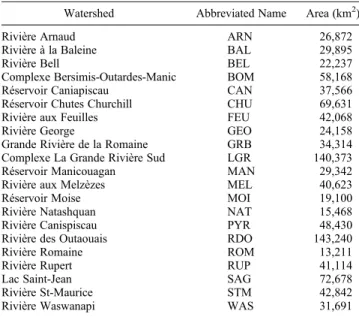
[33] Figure 6 shows the spread, in terms of CV, among the
NCEP-driven RCM simulations, which is a simple quanti-fication of RCM’s structural uncertainty. Though the CV values are small for the majority of the watersheds, they generally increase with return period. For all precipitation Figure 2. Observed regional return levels (in mm) of 10-, 30- and 50-yr return period for 1-, 3- and 7-day
duration-return period combinations considered, the south-ernmost and eastsouth-ernmost watersheds are associated with relatively larger values of CV suggesting larger structural uncertainty for these watersheds compared to northern ones. [34] To assess the uncertainty associated with the driving
AOGCM, we now turn to the two RCMs that have been driven by two distinct AOGCMs. It is difficult to adequately quantify the uncertainty associated with the driving AOGCM since only two AOGCMs are used to drive the same RCM. Nevertheless, CV for both RCM3 and CRCM (figure not shown) provides a rough estimate of this uncer-tainty. The results suggest that compared to structural uncertainty, the uncertainty associated with the driving AOGCM is relatively small. A better quantification of this uncertainty can only be achieved when more AOGCMs are used to drive the same RCM. In similar studies conducted within the ENSEMBLES project [Christensen et al., 2009] over Europe, it was found that the uncertainty associated with the AOGCMs is larger than the structural uncertainty for some variables and seasons.
4.4. Projected Changes
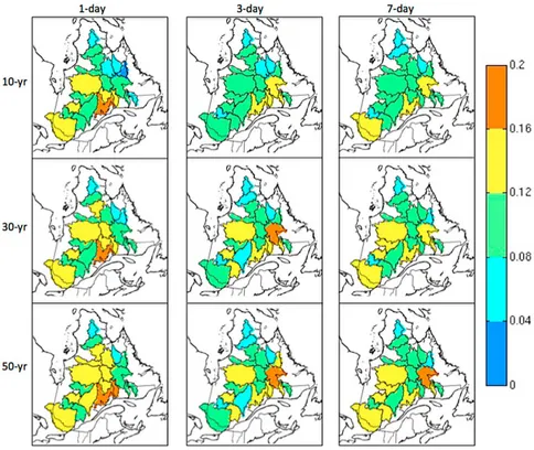
[35] In the present article, projected changes to
precipita-tion extremes are studied at the watershed/regional scale by comparing the selected return levels derived from
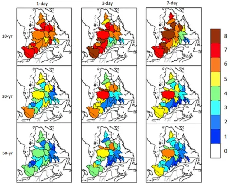
AOGCM-driven simulations for future 2041–70 period with those for the current 1971–2000 period, for the eight AOGCM/RCM pairs. It is assumed here that the frequency distribution remains stationary for the current and future periods. The spatial patterns of current-period AOGCM-driven RCM simulated return levels (figure not shown) is very similar to that of NCEP-driven RCM simulations and observations, with return levels decreasing from south to north. Figure 7 shows ensemble-averaged projected changes to 10-, 30-and 50-yr return levels of 1-, 3- 30-and 7-day precipitation extremes for the future 2041–70 period with respect to the current 1971–2000 period. An increase in return levels in future climate is projected for nearly all watersheds, with relatively smaller (positive/negative) changes for some of the southeasternmost watersheds. One- and 3-day return levels are associated with larger increases compared to 7-day cases. Average change for all watersheds, return periods and precipitation durations is of the order of 13%, with minimum changes in the 5 to 9% range for the southeastern watersheds ROM, NAT, CHU and MOI, while maximum changes of the order of 16 to 18% is noted for the northern watersheds (ARN, BAL, FEU, PYR and MEL).
[36] Figures 8 and 9 show CRCM projected changes,
when driven by CCSM and CGCM3, respectively. While the mean changes for all watersheds lie in the 7% range for Figure 3. Relative difference between Q(1,10)derived from NCEP-driven RCM simulations and observed
data set for 14 of the 21 watersheds for the reference 1980–2000 period. Ensemble averaged differences are also shown.
CRCM_CCSM, it is around 18% for CRCM_CGCM3. Nevertheless, for both, highest increases in return values are found for short-duration precipitation extremes compared to longer duration extremes. While CRCM_CCSM suggests decreases in return values for the southeastern watersheds, it is not as widespread for CRCM_CGCM3. The largest increases are found for the three northernmost watersheds, ARN, FEU and MEL with CRCM_CGCM3 for most of the return levels presented in Figure 9, while it varies with the duration of precipitation extremes for CRCM_CCSM. Thus, though the climate-change signal appears to be consistent for most of the watersheds (with the exception of some eastern and southwestern watersheds), important differences in magnitude can be noted between CRCM_CGCM3 and CRCM_CCSM projections. Similar to the case of CRCM, noticeable difference is found in the magnitude of projec-tions for the two RCM3 simulaprojec-tions with average projected increase of 9% for RCM3_CGCM3 and 16% for RCM3_GFDL. The above comparison highlights the need to use several AOGCMs at the boundaries to assess the uncertainty associated with the driving AOGCM.
[37] Figure 10 shows the CV (defined in the methodology
section) associated with projected changes to regional return
levels for the multi-RCM ensemble. Coefficient of variation is a useful measure in associating a level of confidence with projected changes for the studied watersheds. The value of CV for projected changes to Q(1,10)is less than 1.0 for all
watersheds, suggesting relatively high confidence in the projections for this return level for all watersheds. In all cases, larger CVs are noted for eastern watersheds (CHU, GEO, MOI, NAT and ROM), particularly for higher return periods and precipitation durations, suggesting lower level of confidence in the projections for these watersheds.
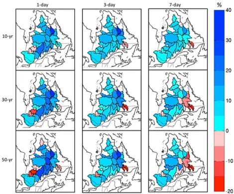
[38] The statistical significance of projected changes to
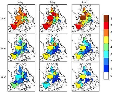
single- and multiday precipitation extremes from current to future climate is assessed at 5 and 10% significance levels (see Figures 11 and 12, respectively) using the nonpara-metric vector bootstrap approach described in the method-ology section. These figures show the number of RCM_AOGCM pairs that suggest statistically significant changes. These results are also summarized in Table 3 for each return period and precipitation duration combination. Majority of the 8 RCM_AOGCM pairs suggest significant increases in 10-yr return levels of single- and multiday extremes. The number of RCM_AOGCM pairs that suggest significant changes is generally limited to 3–5 range for the Figure 4. Relative difference between Q(7,50)derived from NCEP-driven RCM simulations and observed
data set for 14 of the 21 watersheds for the reference 1980–2000 period. Ensemble averaged differences are also shown.
southeastern watersheds. With increasing return period, a drop in the number of pairs that suggest significant changes is obvious in Figures 11 and 12. Clearly, more number of RCM_AOGCM pairs suggests significant changes at 10% significance level for all cases shown in these figures. It should be noted that negative changes to selected return
levels are not found statistically significant for any of the watershed.
[39] Finally, it is important to mention that projected
changes to precipitation extremes were studied earlier by Mladjic et al. [2011] and Mailhot et al. [2012] for large Canadian climatic regions. Though the results of the present Figure 5. Scatterplots of 10- (red), 30- (blue) and 50-yr (green) return levels (in mm) of 1-, 3- and 7-day
precipitation extremes for the 1980–2000 period. x axis corresponds to NCEP driven RCM simulation, while y axis corresponds to AOGCM driven simulation. Numbers in each panel represent average percent-age difference between the NCEP and AOGCM driven simulations.
Figure 6. Coefficient of variation of NCEP-driven RCM simulations to 10-, 30- and 50-yr regional return levels of 1-, 3- and 7-day precipitation extremes.
Figure 7. Ensemble averaged projected changes (in %) to 10-, 30- and 50-yr regional return levels of 1-, 3- and 7-day precipitation extremes for future 2041–2070 period with respect to the current 1971–2000 period.
Figure 8. Projected changes (in %) to 10-, 30- and 50-yr regional return levels of 1-, 3- and 7-day pre-cipitation extremes for future 2041–2070 period with respect to the current 1971–2000 period for CRCM_CCSM.
Figure 9. Projected changes (in %) to 10-, 30- and 50-yr regional return levels of 1-, 3- and 7-day pre-cipitation extremes for future 2041–2070 period with respect to the current 1971–2000 period for CRCM_CGCM3.
Figure 10. Coefficient of variation of projected changes to 10-, 30- and 50-yr regional return levels of 1-, 3- and 7-day precipitation extremes based on the multi-RCM ensemble. Blue (red) dots are used for water-sheds with positive (negative) projected ensemble averaged changes.
Figure 11. Number of AOGCM/RCM simulation pairs (out of eight) that predict a significant change (at 5% level) for 10-, 30- and 50-yr regional return levels of 1-, 3- and 7-day precipitation extremes.
study agree in general with those of the above two studies, important spatial patterns of projected change emerged by performing watershed level analyses.
5.
Summary and Conclusions
[40] An evaluation of single- and multiday (i.e., 1-, 2-, 3-,
5-, 7-, and 10-day) precipitation characteristics, and their projected changes are assessed using a multi-RCM ensemble for 21 northeast Canadian watersheds covering mainly the Quebec province of Canada. The precipitation character-istics considered are 10-, 30- and 50-yr return levels of single- and multiday precipitation extremes, which are modeled for the selected watersheds using the RFA approach [Hosking and Wallis, 1997]. The multi-RCM ensemble is provided by NARCCAP and we consider six different RCMs and their simulations. The simulations considered in this study include six NCEP-driven RCM simulations for the 1980–2000 period and eight pairs of AOGCM-driven RCM simulations for current (1971–2000) and future (2041–70) periods following the SRES A2 scenario. A gridded data set
of daily precipitation available at 10 km resolution from Hydro-Quebec is used for evaluation purposes.
[41] Statistical homogeneity of the 21 watersheds used in
the study is verified following regional homogeneity tests devised by Hosking and Wallis [1997]. This is followed by the selection of a best fitting distribution for each of the watersheds as well as an overall best fitting distribution for the entire study area. The GEV distribution is picked as the overall best fitting distribution, from among the five candi-date distributions (GNO, GEV, GLO, PE3 and GPA). Per-formance errors associated with various RCMs and simple quantification of RCM structural uncertainty, followed by the effect of boundary conditions and projected changes to 10-, 30- and 50-yr return levels of 1-, 3- and 7-day precipi-tation extremes are analyzed. An attempt is made to associ-ate some level of confidence with projected changes to return levels for various watersheds followed by an assess-ment of statistical significance of projected changes.
[42] From the analyses presented in this paper, the
fol-lowing main conclusions can be drawn:
[43] 1. Comparison of 10-, 30- and 50-yr return levels,
derived from NCEP-driven RCM simulations, against those derived from observed data set suggests positive perfor-mance errors for most of the RCMs (except for CRCM) for low return period and short duration extremes. The CRCM generally underestimates observed return values. Neverthe-less, for higher return period and longer duration cases, the tendency is less obvious as nearly half of the RCMs under-estimate the return values. Based on the average absolute differences between observed and RCM simulated return levels, WRFG performs better compared to other RCMs for the precipitation characteristics considered in this study, followed closely by RCM3 and MM5I. Ensemble-averaged return-values, in general, are found to be close to those Figure 12. Number of AOGCM/RCM simulation pairs (out of eight) that predict a significant change
(at 10% level) for 10-, 30- and 50-yr regional return levels of 1-, 3- and 7-day precipitation extremes.
Table 3. Percentage of Statistically Significant Changes for 10-, 30- and 50-Year Regional Return Levels of 1-, 3-, and 7-Day Pre-cipitation Extremes at the 95% Level (With 90% Level in Parentheses)
Return Period
Precipitation Duration
1-Day 3-Day 7-Day
10-year 75 (79) 37 (49) 29 (37)
30-year 72 (76) 44 (55) 34 (43)
obtained with RCM3, WRFG and MM5I, for most of the watersheds.
[44] 2. In a similar manner, lateral boundary forcing
errors, obtained by comparing return levels derived from NCEP-driven and AOGCM-driven simulations, suggest smaller difference compared to performance errors. In gen-eral, the lateral boundary forces errors are less than 10% between the two simulations (AOGCM versus NCEP driven).
[45] 3. Structural uncertainty, represented by the spread of
the NCEP-driven RCM simulations, i.e., CV, is in general less than 0.2 for all watersheds, for all precipitation duration-return period combinations considered. Concerning RCM uncertainty associated with the driving AOGCM, results based on CRCM and RCM3 simulations, both driven by two different AOGCMs, suggest smaller uncertainties compared to the structural uncertainty.
[46] 4. In general, all simulations indicate an increase in
return levels with important differences between models. Overall, larger projected changes are found for northern watersheds, while the smallest projected changes are found for southeastern watersheds. Even though negative changes of larger percentage are noted for individual models, the majority of these changes are within the 0–5% range. The largest increase (19%) is associated with HRM3_HADCM3, which is also associated with largest differences for perfor-mance errors and choice of boundary conditions. A similar observation is noted for ECP2_GFDL case that is associated with the smallest change (6%).
[47] 5. The CV, used to assess confidence in projected
changes, suggests low-confidence for southeastern water-sheds (especially CHU, MOI, NAT, and ROM). This is par-ticularly true for higher return periods of longer duration precipitation extremes. Consequently, the number of RCM/ AOGCM pairs suggesting significant changes for these watersheds are generally limited to one or two.
[48] In regions with significant changes in precipitation
extremes, environment and society would be impacted, e.g., combined sewer systems and management of flood control structures in fast responding areas and water storage sys-tems. The results of the present study would be useful for designing future hydroelectric facilities in Quebec province of Canada.
[49] When the entire NARCCAP project will be
com-pleted, investigation using a larger and complete multi-RCM ensemble will be possible, with 12 (instead of eight) refer-ence and future-period simulations. Future improvements of model parameterization and changes in scenario develop-ment may produce different, perhaps better, estimates than the ones presented in this study. It will also be interesting to explore the physical mechanisms responsible for the changes in precipitation extremes similar to for example Jaeger and Seneviratne [2011].
[50] Acknowledgments. This research was undertaken as part of a Collaborative Research and Development (CRD) project funded by the Nat-ural Sciences and Engineering Research Council (NSERC) of Canada, Hydro-Quebec and Ouranos Consortium. The authors would like to thank Dominique Tapsoba, from Hydro-Quebec, for providing gridded observed precipitation data set, NARCCAP project team for the RCM-simulated pre-cipitation data used in this study and three anonymous referees for their helpful comments. The first author would like to thank Debasish PaiMa-zumder and Bratislav Mladjic for technical assistance.
References
Alley, R. B., et al. (2007), Summary for policymakers, in The Physical Science Basis. Contribution of Working Group 1 to the Fourth Assessment Report of the Intergovernmental Panel on Climate Change, edited by S. Solomon et al., pp. 1–18, Cambridge Univ. Press, Cambridge, U. K.
Beniston, M., et al. (2007), Future extreme events in European climate: An exploration of regional climate model projections, Clim. Change, 81, 71–95, doi:10.1007/s10584-006-9226-z.
Brown, R. D. (2010), Analysis of snow cover variability and change in Québec, 1948–2005, Hydrol. Processes, 24(14), 1929–1954.
Christensen, J. H., and O. B. Christensen (2003), Severe summertime flood-ing in Europe, Nature, 421, 805–806, doi:10.1038/421805a.
Christensen, J. H., T. R. Carter, M. Rummukainen, and G. Amanatidis (2007), Evaluating the performance and utility of regional climate mod-els: The PRUDENCE project, Clim. Change, 81, 1–6, doi:10.1007/ s10584-006-9211-6.
Christensen, J. H., M. Rummukainen, and G. Lenderink (2009), Formula-tion of very-high-resoluFormula-tion regional climate model ensembles for Europe, in ENSEMBLES: Climate Change and Its Impacts: Summary of Research and Results From the ENSEMBLES Project, edited by P. Van der Linden and J. F. B. Mitchell, pp. 47–58, Met Off. Hadley Cent., Exeter, U. K.
Crétat, J., and B. Pohl (2012), How physical parameterizations can modu-late internal variability in a Regional Climate Model, J. Atmos. Sci., 69, 714–724, doi:10.1175/JAS-D-11-0109.1.
Davison, A. C., and D. V. Hinkley (1997), Bootstrap Methods and Their Application, 582 pp., Cambridge Univ. Press, Cambridge, U. K. de Elía, R., D. Caya, H. Côté, A. Frigon, S. Biner, M. Giguère, D. Paquin,
R. Harvey, and D. Plummer (2008), Evaluation of uncertainties in the CRCM-simulated North American climate, Clim. Dyn., 30, 113–132, doi:10.1007/s00382-007-0288-z.
De Sales, F., and Y. Xue (2010), Assessing the dynamic downscaling abil-ity over South America using the intensabil-ity-scale verification technique, Int. J. Climatol., 31, 1205–1221, doi:10.1002/joc.2139.
Di Luca, A., R. de Elia, and R. Laprise (2011), Potential for added value in precipitation simulated by high resolution nested Regional Climate Models and observations, Clim. Dyn., 38, 1229–1247, doi:10.1007/ s00382-011-1068-3.
Efron, B., and R. J. Tibshirani (1993), An Introduction to the Bootstrap, 436 pp., Chapman and Hall, London.
Emori, S., and S. J. Brown (2005), Dynamic and thermodynamic changes in mean and extreme precipitation under changed climate, Geophys. Res. Lett., 32, L17706, doi:10.1029/2005GL023272.
Feser, F. (2006), Enhanced detectability of added value in limited-area model results separated into different spatial scales, Mon. Weather Rev., 134, 2180–2190, doi:10.1175/MWR3183.1.
Fowler, H. J., M. Ekström, C. G. Kilsby, and P. D. Jones (2005), New esti-mates of future changes in extreme rainfall across the UK using regional climate model integrations. 1. Assessment of control climate, J. Hydrol., 300(1–4), 212–233, doi:10.1016/j.jhydrol.2004.06.017.
Groupe de Recherche en Hydrologie Statistique (1996), Presentation and review of some methods for regional flood frequency analysis, J. Hydrol., 186, 63–84, doi:10.1016/S0022-1694(96)03042-9.
Haberlandt, U. (2007), Geostatistical interpolation of hourly precipitation from rain gauges and radar for a large-scale extreme rainfall event, J. Hydrol., 332, 144–157, doi:10.1016/j.jhydrol.2006.06.028.
Heinrich, G., and A. Gobiet (2011), Uncertainty assessment of the reclip: century ensemble, Final Rep. Part D, Wegener Cent. for Clim. and Global Change, Inst. for Geophys., Astrophys., and Meteorol., Univ. of Graz, Graz, Austria. [Available at http://www.uni-graz.at/en/igam7www_heinrich_ gobiet-2011-wegcreporttoacrp-reclip_climatechangeuncertaintyalps.pdf.] Hofstra, N., M. New, and C. McSweeney (2010), The influence of
interpo-lation and station network density on the distributions and trends of cli-mate variables in gridded daily data, Clim. Dyn., 35(5), 841–858, doi:10.1007/s00382-009-0698-1.
Hosking, J. R. M., and J. R. Wallis (1997), Regional Frequency Analysis, 224 pp., Cambridge Univ. Press, Cambridge, U. K., doi:10.1017/ CBO9780511529443.
Jaeger, E. B., and S. I. Seneviratne (2011), Impact of soil moisture-atmosphere coupling on European climate extremes and trends in a regional climate model, Clim. Dyn., 36, 1919–1939, doi:10.1007/s00382-010-0780-8. Jeannée, N., and D. Tapsoba (2010), Improved mapping of daily precipita-tion over Quebec using the moving-geostatistics approach, paper presented at GeoENV 2010, Ghent Univ., Ghent, Belgium. [Available at http://www. geovariances.com/en/IMG/pdf/Abstract-GeoEnv2010-JeanneeTapsoba.pdf.] Khaliq, M. N., T. B. M. J. Ouarda, L. Sushama, and P. Gachon (2009), Identification of hydrological trends in the presence of serial and cross correlations: A review of selected methods and their application to annual
flow regimes of Canadian rivers, J. Hydrol., 368, 117–130, doi:10.1016/j. jhydrol.2009.01.035.
Mailhot, A., I. Beauregard, G. Talbot, D. Caya, and S. Biner (2012), Future changes in intense precipitation over Canada assessed from multi-model NARCCAP ensemble simulations, Int. J. Climatol., doi:10.1002/joc.2343, in press.
May, W. (2008), Potential future changes in the characteristics of daily pre-cipitation in Europe simulated by the HIRHAM regional climate model, Clim. Dyn., 30, 581–603, doi:10.1007/s00382-007-0309-y.
Mearns, L. O., W. J. Gutowski, R. Jones, L.-Y. Leung, S. McGinnis, A. M. B. Nunes, and Y. Qian (2009), A regional climate change assessment pro-gram for North America, Eos Trans. AGU, 90, 311–312, doi:10.1029/ 2009EO360002.
Mladjic, B., L. Sushama, M. N. Khaliq, R. Laprise, D. Caya, and R. Roy (2011), Canadian RCM projected changes to extreme precipitation char-acteristics over Canada, J. Clim., 24, 2565–2584, doi:10.1175/ 2010JCLI3937.1.
Nikulin, G., E. Kjellström, U. Hansson, G. Strandberg, and A. Ullerstig (2011), Evaluation and future projections of temperature, precipitation and wind extremes over Europe in an ensemble of regional climate simulations, Tellus, Ser. A, 63(1), 41–55, doi:10.1111/j.1600-0870.2010.00466.x. Poitras, V., L. Sushama, F. Segleniek, M. N. Khaliq, and E. Soulis (2011),
Projected changes to streamflow characteristics over western Canada as
simulated by the Canadian RCM, J. Hydrometeorol., 12, 1395–1413, doi:10.1175/JHM-D-10-05002.1.
Prömmel, K., B. Geyer, J. M. Jones, and M. Widmann (2010), Evaluation of the skill and added value of a reanalysis-driven regional simulation for Alpine temperature, Int. J. Climatol., 30, 760–773, doi:10.1002/ joc.1916.
Seth, A., S. Rauscher, S. Camargo, J.-H. Qian, and J. Pal (2007), RegCM regional climatologies for South America using reanalysis and ECHAM model global driving fields, Clim. Dyn., 28, 461–480, doi:10.1007/ s00382-006-0191-z.
Tapsoba, D., V. Fortin, F. Anctil, and M. Hache (2005), Apport de la tech-nique du krigeage avec dérive externe pour une cartographie raisonnée de l’équivalent en eau de la neige. Application aux bassins de la rivière Gatineau, Can. J. Civ. Eng., 32(1), 289–297, doi:10.1139/l04-110. Tebaldi, C., J. M. Arblaster, K. Hayhoe, and G. A. Meehl (2006), Going to
the extremes: An intercomparison of model-simulated historical and future changes in extreme events, Clim. Change, 79, 185–211, doi:10.1007/s10584-006-9051-4.
Trenberth, K. E., A. Dai, R. M. Rasmussen, and D. B. Parsons (2003), The changing character of precipitation, Bull. Am. Meteorol. Soc., 84, 1205–1217, doi:10.1175/BAMS-84-9-1205.