D
OCUMENT DE
T
RAVAIL
DT/2002/12
The medium and long term effects of
an expansion of education on poverty
in Côte d’Ivoire
A dynamic microsimulation study
THE MEDIUM AND LONG TERM EFFECTS
OF AN EXPANSION OF EDUCATION ON POVERTY IN COTE D’IVOIRE A DYNAMIC MICROSIMULATION STUDY
Michael Grimm*
(DIAL – UR CIPRE de l’IRD Institut d’Etudes Politiques de Paris)
Document de travail DIAL / Unité de Recherche CIPRE Octobre 2002
RESUME
J’utilise un modèle de micro-simulation dynamique pour analyser les effets distributifs d'une expansion de l'éducation en Côte d'Ivoire à moyen et long terme (1998-2015). Les simulations sont effectuées, selon plusieurs politiques actuellement en place ou en discussion dans ce pays. Des hypothèses variées concernant l'évolution du rendement de l'éducation et de la demande de travail sont examinées. Les effets directs entre éducation et revenu comme les différents canaux de transmission, tels que les choix d'activité, la fécondité et la composition des ménages sont analysés. Les effets de l'expansion de l'éducation sur la croissance des revenus des ménages, la distribution du revenu et la pauvreté dépendent de manière cruciale de l'hypothèse faite concernant l'évolution du rendement de l'éducation et de la demande de travail. Si le rendement de l'éducation reste constant et le marché du travail segmenté, les effets seront relativement modérés.
ABSTRACT
I use a dynamic microsimulation model to analyse the distributional effects of an expansion of education in Côte d'Ivoire in the medium and long term (1998-2015). The simulations are performed in order to replicate several policies in force or subject to debate in this country. Various hypotheses concerning the evolution of returns to education and labour demand are tested. The direct effects between education and income as well as the different transmission channels, such as occupational choices, fertility, and household composition, are analysed. The effects of the educational expansion on the growth of household incomes, their distribution and poverty depend very crucially on the hypothesis made on the evolution of returns to education and labour demand. If returns to education remain constant and the labour market segmented, the effects will be very modest.
*
I thank Denis Cogneau for very useful comments and discussions. The labour supply and earnings model used in this study was constructed jointly with Denis Cogneau. It is also used in a paper, where we study the distributional impact of AIDS in Côte d’Ivoire. This working paper is a shorter version of chapter six of my doctoral dissertation. The original text (in French) can be obtained upon request by the author.
Content
Introduction 4
1. Education in Côte d’Ivoire 5
1.1. Education system and education policy since independence 5
1.2. Enrolment ratios and education level 5
1.3. Current education programmes 6
2. Model structure 6
2.1. Key characteristics of the model 6
2.2. Modelling of schooling decisions 7
2.3. Modelling of occupational choices and earnings 7
2.4. Transmission channels between education and income distribution in the model 10
3. Policy experiments 10
4. Results 12
4.1. Evolution of the level and the distribution of education 12
4.2. Impact on growth and the distribution of income 14
4.3. Indirect effects through the different transmission channels 17
5. Conclusion 19
Endnotes 19
References 20
Appendix 22
List of tables
Table 1. Illiteracy rates 5
Table 2. Enrolment ratios 6
Table 3. Summary of the policy experiments 11
Table 4. Illiteracy rate and average years of schooling 13
Table 5. Average years of schooling by birth cohort simulated for Côte d’Ivoire for 2015
and observed for some other countries and regions in the 1990s 13
Table 6. Income, inequality and poverty 15
Table 7. Employment structure, individuals older than 11 years, not enrolled 18 Table 8. Total fertility rate (TFR), mean household size, and dependency ratio 18 Table A1. Probit estimations of the probability of being enrolled in t conditional on the state
in t-1 22
Table A2. Observed and simulated enrolment ratios in 1998 24
Table A3. Agricultural profit function 24
Table A4. Activity choice and labour income model 25
List of figures
Figure 1. Level and inequality of household income per capita 16 Figure 2. Relative changes of mean household income per capita by percentiles 17
INTRODUCTION
Today it is widely recognized that human capital, in particular that acquired by schooling, is a key factor of development. The link is clearly established at the micro-economic level. Individuals with more education receive in average more income [e.g., Mincer, 1974; Schultz 1994, 1999]. This implies that a more egalitarian distribution of education may constitute an efficient mean to reduce inequality of income distribution. At the macro-economic level, the “new growth theory”, pioneered by Lucas [1988] and Romer [1990], suggests that the accumulation of human capital may have externalities which drive the economy on a continuous growth path. However, empirically the link seems less clear. Whereas Krueger and Lindahl [2000] find that faster growth of the human capital stock also leads to faster growth of per capita income, other authors are more sceptic. Pritchett [2001], for instance, claims that a rise of education can only play the “engine of growth”-role if that rise is accompanied by higher demand for education, if education satisfies a certain quality standard, and if education is not allocated to socially inefficient tasks. Education is thus viewed as a necessary, but not sufficient condition, or as Pritchett writes: “Education is no magic bullet”. Benhabib and Spiegel [1994], and more recently Bils and Klenow [2000] even deny completely this link putting forward the argument of inverse causality, i.e. that economic growth accelerates human capital investments and not the other way around.
In any case, beside the link from education to income, one attributes numerous positive external effects to education, in particular to women’s education: less, healthier, and better educated children, higher autonomy of women, and increased labour supply outside the household [e.g.,
Cleland and Rodriguez, 1988; Jejeebhoy, 1995; Schultz, 1997]. Some authors even argue that an
improvement of women’s situation may be a source of economic growth [e.g., Behrmann Foster,
Rosenzweig et al., 1999; Blackden and Bhanu, 1999; Forsythe, Korzeniewicz and Durrant, 2000; Klasen, 1999]. Likewise, in the Millennium Development Goals education is seen as a powerful
instrument not only “for reducing poverty and inequality”, but also “for improving health and social well-being, laying the basis for sustained economic growth, and being essential for building democratic societies and dynamic, globally competitive economies” [United Nations, 2000].
Whereas East and South-East Asia as well as Latin America experienced significant progress in terms of education over the last decades, Sub-Saharan Africa is still far behind. This region has the lowest enrolment ratios at each level and the average African adult has acquired less than three years of schooling [World Bank, 2001]. From a political point of view, it is therefore interesting to analyse the effects in the medium and long term of a significant expansion of education in Sub-Saharan Africa on income distribution and poverty. What would be the magnitude of the direct effects between education and income. What would be the role of the different transmission channels, such as fertility, age at marriage, formation and composition of households, and labour supply? The purpose of this article is to address these questions for the case of Côte d’Ivoire using a dynamic microsimulation model. The simulations consider policies which are in force or subject to debate in this country. Their impact on household incomes and their distribution is examined from 1998 until 2015 under several assumptions concerning the evolution of labour demand and returns to education.
In contrast to Ferreira and Leite (2002) the used model accounts for the dynamic features of the problem. Ferreira and Leite (2002), who analyse the case of the Ceará Region (Brazil), work with a constant population structure. Among the demographic variables, such as fertility, mortality, migration and marriage, only the distribution of education and the size of the households is taken into account. This gives the exercise a very hypothetical character and risks to bias strongly the results. Furthermore, their analysis is comparative static, therefore it does not allow to reproduce the trajectory between the point of departure and arrival of individuals and households.
Section 1 summarizes very briefly the education policy and the evolution of the distribution of education in Côte d‘Ivoire. Section 2 presents the used microsimulation model and its main transmission channels between education and income distribution. Section 3 outlines the policy experiments which are simulated. Section 4 analyses the simulation results. Section 5 concludes.
1. EDUCATION IN CÔTE D’IVOIRE
1.1. Education System and Education Policy since Independence
The education system in Côte d’Ivoire is based on the model inherited from the French colonial era. School starts normally at five, but many children enter later. Children stay in primary school for a total of six years then move to junior secondary school (four years) and to upper secondary school (three years). Entrance to junior secondary school is permitted upon success to the “Certificat
d’Etudes Primaires et Elementaire” (CEPE) examination and access to upper-secondary school is
controlled by the “Brevet d’Etudes du Premier Cycle” (BEPC). At the end of secondary school, each student has to pass the “Baccalauréat” examination before going to university. Professional training and technical education is situated mainly on the secondary level [Kouadio and Mouanda,
2001].
After independence, Côte d’Ivoire allocated approximately 40% of public expenditures to education, more than twice the share allocated in Burkina Faso or Senegal. However, with the onset of the economic crisis in the beginning of the 1980s, this share decreased progressively preventing an improvement of the efficiency of the school system which was already judged as not satisfactory. A large part of education expenditures have been used for salaries. Primary school has been systematically neglected. This explains to some extend why a large part of the population, in particular rural and female, have received no education. Furthermore, repetition rates of 30% are not seldom and only about 35% pass successfully the BEPC [Cogneau and Mesplé-Somps, 2002]. 1.2. Enrolment Ratios and Education Level
The following descriptive statistics are based on two household surveys, the “Enquête Prioritaire” of 1993 and the “Enquête de Niveau de Vie” of 1998 (called “EP 1993” and “ENV 1998” hereafter), both carried out by the Institut National de la Statistique de la Côte d'Ivoire (INS) and the World Bank.
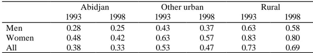
TABLE 1 ILLITERACY RATES (population 15 years and older)
Abidjan Other urban Rural 1993 1998 1993 1998 1993 1998
Men 0.28 0.25 0.43 0.37 0.63 0.58
Women 0.48 0.42 0.63 0.57 0.83 0.80
All 0.38 0.33 0.53 0.47 0.73 0.69
Source: EP 1993, ENV 1998; computations by the author.
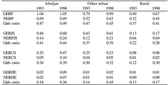
Table 1 shows that a large part of the Ivorian population is still not able to read and write. Illiteracy is particularly high in rural areas and for women. However, the evolution between 1993 and 1998 shows that illiteracy decreases. The enrolment ratios also show a significant inequality between cities and rural areas. One can also state an abrupt fall of enrolment ratios after primary school and a strong difference between gross and net enrolment ratios.1 This difference can be explained by delayed entries in the schooling system, frequent schooling interruptions, and high repetition rates, in particular during the last two years of primary schooling. Girls are strongly
underrepresented in secondary school and university. However, enrolment ratios increase at all schooling levels.2
TABLE 2 ENROLMENT RATIOS
Abidjan Other urban Rural
1993 1998 1993 1998 1993 1998 GERP 1.04 1.05 0.79 0.99 0.49 0.67 NERP 0.69 0.69 0.52 0.63 0.32 0.45 Girls -ratio 0.47 0.49 0.47 0.45 0.37 0.41 GERJS 0.46 0.60 0.43 0.61 0.13 0.17 NERPJS 0.14 0.24 0.12 0.21 0.04 0.04 Girls -ratio 0.41 0.44 0.37 0.39 0.22 0.28 GERUS 0.25 0.47 0.25 0.23 0.08 0.08 NERUS 0.05 0.10 0.04 0.05 0.01 0.02 Girls -ratio 0.36 0.39 0.30 0.32 0.12 0.30 GERHE 0.03 0.09 0.01 0.02 0.01 0.01 NERHE 0.02 0.07 0.01 0.01 0.00 0.00 Girls -ratio 0.18 0.36 0.14 0.45 0.13 0.17
Notes: GERP/NERP=Gross/net enrolment ratio in primary school; GERJS/NERJS=Gross/net enrolment ratio in
junior secondary school; GERUS/NERUS= Gross/net enrolment ratio in upper secondary school; GERHE/NERHE= Gross/net enrolment ratio in higher education.
Source: EP 1993, ENV 1998; computations by the author.
1.3. Current education programmes
The current education policy of Côte d’Ivoire focuses principally on three objectives [INS, 2001]3: first, to achieve almost universal primary school enrolment, according to the aim fixed at the “World Conference on Education for All”, held in Jomtien, Thailand in 1990; second, to reduce gender inequality in terms of education; and third, to literate the adult population. The means by which the Ivorian authorities want to achieve these objectives are mainly orientated to the supply side. They contain, among others things, the construction of primary schools and education centres for adults, the reorganisation of education management, the pre-service and in-service training of teachers, the larger distribution of schooling materials such as textbooks, and the revision of curriculum content and implementation. These measures are supported by several Word Bank programmes [see World Bank, 2002a, 2002b].
2. MODEL STRUCTURE
2.1. Key characteristics of the model
I use a dynamic microsimulation model designed to simulate at the individual level the most important demographic and economic events through time. The microsimulation approach allows to take into account individual heterogeneity, in particular regarding the capacity of accumulating human capital and earning income. Furthermore, it allows to analyse the policy outcomes in terms of inequality and poverty, and not only in terms of growth, as does an aggregated model. The dynamic approach is important to account for the time it takes to accumulate human capital and the occurring interactions with other economic and demographic variables during this period. The used model is similar to simulation models used in industrialized countries to analyse pension reforms, the distribution of life-cycle incomes, or the accumulation of wealth.4 The base unit is the individual, but each individual belongs in each period to a specific household. The model is a discrete time model. Each period corresponds to one year. I assume a fixed order concerning the different events: marriage, household formation, school enrolment, fertility, mortality, international
immigration, reallocation of land, occupational choices, generation of individual earnings and household income. The population of departure is constructed using the EP 1993. This survey contains information about the socio-demographic characteristics of households and its members, their housing, education, employment, agricultural and non-agricultural enterprises, earnings, expenditures, and assets. From March to June 1992, 1680 households in Abidjan (economic capital of Côte d'Ivoire), and from June to November 1993 7920 households from the rest of the country (among them 3360 in other Ivorian towns) were interviewed. The total sample covers 58014 individuals. Then the sample was calibrated on January 1st 1993. In what follows I present briefly the modelling of schooling, occupational choices, and earnings which constitute the central modules of the model. The modelling of the other behaviours is presented in appendix.
2.2. Modelling of schooling decisions
I use the information about current enrolment and enrolment in the previous year in the EP 1993 and the ENV 1998 to estimate transition rates into and out of schooling. The models are estimated separately for boys and girls five to 25 years old using age, household composition, Ivorian citizenship, educational level already attained, matrimonial status, relation to the household head, land owned by the household, region of residence, and educational attainment of the father and the mother as explicative variables. The estimated coefficients of the corresponding probit models as well as a comparison of observed and simulated enrolment ratios for 1998 figure in Tables A1 and A2 in appendix. They show that the probability of school entry depends, as one can expect, strongly on age. It is higher for children with educated parents (notably for girls), and is smaller for children in Non-Ivorian households. Furthermore, the probability of entry is higher if the child has already acquired some education in the past. The probability of staying in school depends positively on the educational level already attained, negatively on marriage and the quantity of land owned by the household, and is higher in urban areas, especially Abidjan. During the simulation, enrolment status is updated in each period for all children from five to 25 years old using the estimated coefficients and either a Monte Carlo lottery5 or fixed progression rates imposed according to the performed policy experiment. In the latter case, the estimated parameters are used to select the children with the highest empirical probability to experience the respective transition. As mentioned above, repetition of classes is very frequent in Côte d'Ivoire, especially before the entry into junior secondary school. To account for this phenomenon, I fixed the repetition rates at 20% for the fifth year of primary school, at 50% for the sixth year of primary school and at 10% for all other classes.
2.3. Modelling of occupational choices and earnings
The labour income model draws from Roy's model [1951] as formalized by Heckman and Sedlacek [1986]. It is competitive in the sense that no segmentation or job rationing prevail, but only weakly, because labour mobility across sectors does not equalize returns to observed and unobserved individual characteristics. The model is estimated using the EP 1993. It is assumed that each individual older than eleven years and out of school faces three kinds of work opportunities: (i) family work, (ii) self-employment, (ii) wage work. Family work includes all kinds of activities under the supervision of the household head, that is family help in agricultural or informal activities, but also domestic work, non-market labour and various forms of declared “inactivity”. Self-employment corresponds to informal independent activities. In agricultural households (households where some independent agricultural activity is done), the household head may be considered as a self-employed worker bound to the available land or cattle. Wage work concerns dependent employment principally in the formal public and private sectors.
To both, non-agricultural self-employment and wage-work, individual potential earnings functions are associated which only depend on individual characteristics and on task prices:
ln w2i = ln p2+X2i β2+t2i (2)
To family work, an unobserved individual value is associated that depends also on household characteristics, and on other members’ labour supply decisions:
ln w0i = (X0i,Z0h)β0 + t0i (3)
To farming households, a reduced farm profit function derived from a Cobb-Douglas technology is associated:
ln Π0h = ln p0 + α ln Lh + Zhθ + u0h (4)
Then, when the household head is a farmer, secondary members may participate in farm work and therefore w0i is assumed to depend on the “individual’s contribution” to farm profits. This contribution is evaluated while holding fixed other members decisions and the global factor productivity of the farm u0h:
ln ∆Π0i = ln p0 + ln (Lαh+i - Lαh-i) + Zhθ + u0h (5)
where Lh+i = Lh and Lh-1 = Lh – 1 if i is actually working on the farm in h, and Lh+i = Lh + 1and Lh-1 =
Lh alternatively.
This means that the labour decision model is hierarchical between the household head and secondary members, and simultaneous “à la Nash” among secondary members (secondary members do not take into account the consequences of their activity choice on that of other secondary members). In the case of agricultural households, one may then rewrite the family work value as follows:
ln w0i = (X0i,Z0h)β0 + γ [ln p0 + ln (Lαh+i - Lαh-i) + Zhθ] + t0i (6)
γ stands for the (non-unitary) elasticity of the value of family work in agricultural households to the price of agricultural products. For non-agricultural household members, w0 may be seen as a pure reservation wage, where the household head's earnings and other non-labour income of the household is introduced in order to account for an income effect on participation in the labour market.
Comparing the respective values attributed to the three labour opportunities, workers allocate their labour force according to their individual comparative advantage:
i chooses family work iff w0i > w1i and w0i > w2i (7)
i chooses self-employment iff w1i > w0i and w1i > w2i (8)
i chooses wage work iff w2i > w0i and w2i > w1i (9)
The following estimation strategy is adopted: (i) For non-agricultural households, the occupational choice/labour income model represented by equations (1) - (3) and the series of selection conditions (7) - (9) is estimated by maximum likelihood techniques; one obtains a bivariate tobit, like in Magnac [1991]. (ii) For agricultural households, a limited information approach is followed: in a first step, the reduced form profit function (4) is estimated, then an estimate for the individual potential contribution to farm production (5) is derived; in a second step, the reservation wage equation (6) is estimated and the individual potential contribution included, and, because of the
small sample of rural wage workers, the wage functions (1) and (2) estimated for non-agricultural households are retained.
Table A4 (appendix) shows the estimation results for non-agricultural household members, including the head. As for education, returns are ordered as expected: the highest in the wage sector with a 17% increase for each additional year, and the lowest in the informal sector with only 7%. The impact of education on the reservation wage lies in-between but close to the self-employment coefficient (10%). Returns to experience are similar in both, the informal and formal sectors, while the reservation value follows an ever increasing parabola. All three values are higher in towns than in rural areas, wages getting a premium in Abidjan. Non-Ivorians have, as expected, a lower reservation value and are discriminated in the wage sector. Other things being equal, they get 26% less than Ivorians, but not in self-employment. This is again the case for women for whom, other things being equal, the competitive potential wage appears as 83% lower than for men. The reservation value for women is 22% lower than for men, but the effect of this variable should not be interpreted in isolation from the variables describing the relation to the head. Indeed household heads tend to participate most of the time and more frequently if they are female, far away followed by spouses. Among household variables which only influence the reservation value, household head's income for secondary members has the expected positive sign, although it is only hardly significant. The number and age structure of children has a small and mixed influence on participation on the labour market. The number of men in working age, but not that of women, tends to decrease participation. Table A3 (appendix) shows the agricultural profit function, associated to the heads of agricultural households. The number of family workers comes out with a coefficient that is consistent with usual values: a doubling of the work force leads to a roughly 50% increase of agricultural profits. The amount of arable land also comes out with a decreasing marginal productivity. Potential experience and sex of the household head are both significant, whereas education of the household did not come out and was withdrawn from the set of explanatory variables. All regions come out with a negative sign with respect to the Savannah region (North), which reflects the low relative prices for cocoa and coffee in contrast to cotton in the year of estimation 1992/93. Table A4 (appendix) shows the estimation results for secondary members of agricultural households. As noted before, self-employment benefit and wage functions have been constrained to be the same as for non-agricultural households. Not surprisingly, people living in towns tend to work more often outside the family. This is also the case for women and immigrants, whatever their relation to the household head. The presence of children has no effect, while the number of working age men in the household still increases the reservation value of an individual. The above defined potential individual contribution to the agricultural profit increases the propensity to work on the farm with a reasonable elasticity of +0.3.
Land is of course a key variable in the generation of agricultural income. Land is attributed in each household to the household head. If the household head leaves the household, for marriage for instance, land is attributed to the new household head. If the first-born boy of a household leaves for marriage, he receives 50% of the household’s land. The land of households which disappear, due to deaths of all its members, is reallocated within each strata among the households without land in equal parts and such that the proportions of households owning land remain constant with respect to 1993. At the end of each period the quantity of land is increased for each household by 3%, which is the approximate natural population growth rate in the model. Households switch to the agricultural sectori.e. become an agricultural householdif the land they own exceeds a certain threshold level which I fixed at 0.1 ha, and in the opposite, they exit the agricultural sectori.e. become a non-agricultural householdif land size falls under this threshold (in the base sample 45.6% of the households are involved in independent agricultural activity (18.3% urban and 81.7% rural) and 54.4% are not (86.9% urban and 13.1% rural).
2.4. Transmission channels between education and income distribution in the model
As a key determinant of wages and non-farm profits, education has, of course, direct effects on household income. Then education determines, beside other individual and household characteristics, activity choices of individuals who compare their potential remunerations in the two market activities with their reservation wage. Given that wage work offers the highest return to education, this activity becomes more and more lucrative when education increases. Furthermore, education influences negatively on fertility. Fertility is a key variable of the reservation wage and modifies the number of consumption units in the household and, in the long term, the quantity of labour supply available in the household. Finally, parental education influences schooling choices of their children and therefore also modifies the income and demographic behaviour of the children’s generation. However, the model does not account for direct effects from education on mortality, and especially from mother’s education on child mortality.
3. POLICY EXPERIMENTS
Three education policies, of which the last in four variants, plus a reference case are simulated. These experiments are in line with the education programmes debated or already in force in Côte d’Ivoire. They are summarized in Table 3 and explained in detail in what follows. The simulations start in 1993 and end in 2015. They are identical for all experiments until 1998.
REFSIM, the reference simulation, consists in maintaining the enrolment ratios at the different schooling levels at those which would Côte d’Ivoire experience if the observed conditions in 1998 persisted, that is 50% of all children having achieved no or less than six years of schooling, 22% having achieved primary education, 20% having achieved junior secondary education, 6% having achieved upper secondary education and a little less than 2% having achieved at least one year of university education. These proportions imply progression rates between the different schooling levels of 40%, 30%, and 30%. The simulation works as follows: In 1998, 50% of all six years old children enter in primary school and stay there for six years until they obtain the CEPE. Those children with the highest empirical probability to be enrolled are selected. This probability is calculated using the estimated equation relating enrolment status to individual and household characteristics (see Table A1, appendix). Then 40% are selected of those having achieved primary school, likewise according to their empirical probability to be enrolled. They will complete junior secondary school. Then the simulation continues in the same way for the following schooling levels. Furthermore, in the reference case as well as in all other simulations, the repetition rates are set to zero from 1998 on.
PRIMED simulates the case of an almost universal primary school by assuming an entry rate of 90% for the generations being six years old in 1998 and younger. The desired net enrolment ratio is attained in 2003 when the sixth cohort enters in primary school. The selection of children and the simulation process works as in the reference case.
HIGHED assumes, in addition to the 90% entry rate into primary school, progression rates between the following schooling levels of 60%, 60%, and 30% instead of 40%, 30%, and 30%.
ALPH completes the former simulation by an adult literacy programme. From 1998 on, in each period 10% of men and 20% of women between 15 and 40 years old and having less than two years of schooling are randomly selected. The literacy programme is supposed to last three years. Then the years of schooling of all participants are set to two. To reduce gender inequality, I choose more women than men. This last experiment is performed under four different assumptions, three concerning the evolution of the return to education and one concerning the evolution of labour demand in the (formal) wage earner sector.
TABLE 3
SUMMARY OF THE POLICY EXPERIMENTS
Schooling Progr. rate 1998 2005 2010 Simulation level from 1998 on GER NER GER NER GER NER
REFSIM Primary 50% 77% 41% 59% 50% 50% 50% Junior S. 40% 33% 7% 34% 25% 20% 20% Upper S. 30% 14% 2% 10% 5% 6% 6% University 30% 2% 2% 2% 2% 2% 2% PRIMED Primary 90% 77% 41% 100% 90% 90% 90% Junior S. 22% 33% 7% 23% 20% 20% 20% Upper S. 30% 14% 2% 5% 3% 6% 6% University 30% 2% 2% 2% 2% 1% 1% HIGHED Primary 90% 77% 41% 100% 90% 90% 90% Junior S. 60% 33% 7% 61% 47% 54% 54% Upper S. 60% 14% 2% 27% 12% 34% 34% University 30% 2% 2% 3% 3% 7% 7% ALPH HIGHED +
From 1998 on, in each period selection of 10% of men and 20% of women between 15 and 40 years old and being illiterate. Duration of programme: three years, then the years of schooling are set to two (literate).
CR Constant return to education.
DR Decreasing return to education: elasticity between the return to education in each sector and the share of the work force having more than five years of schooling of –1/3.
IR Increasing return to education: elasticity between the return to education in each sector and the share of the work force having more than five years of schooling of +1/3.
SM Maintenance of the share of the work force employed in the (formal) wage earner sector at the share simulated for 1997, which is 11.34%.
Note: GER/NER = Gross/net enrolment ratio.
• First, one may think, according to neo-classical theory, that the entry of more and more educated individuals on the labour market reduce the return to education. Bils and Klenow [2000], for instance, found that countries with higher education levels experience lower returns. For example, as years of schooling go from two to six to ten, the implied income growth for one additional year of schooling falls from 21.6%, to 11.4% to 8.5%. In contrast, one may assume that the return to education increases if the expansion of education is accompanied by an increase of demand of education, due to technological progress or international trade, for instance. This last hypotheses was put forward by Katz and Murphy [1992] for the case of the United States. Finally, one may assume that the return to education remains constant [Card, 1995]. For the decreasing-return-Scenario, ALPHDR, I set an elasticity between the return to education in each sector and the share of the work force (20 years and older) having more than five years of schooling to –1/3. That means if that share increases by 1%, the return to education decreases by 0.33%. In the case of increasing returns, ALPHIR, the elasticity is supposed to be +1/3. The share of the work force having more than five years of schooling increases in the simulation ALPH by approximately 3% per year. This implies that the return to education between 1998 and 2015 in the wage earner sector, for instance, increases from 17.1% to 20.5% under the hypothesis of increasing returns and decreases from 17.1% to 14.3% under the hypothesis of decreasing returns. ALPHCR indicates the constant-return-scenario.
• Another variant, ALPHSM, simulates the case of a segmented labour market. As mentioned in Section II (see also Table A4, appendix) more education makes wage work more and more lucrative relative to work in other sectors. However, in the Ivorian context it is less likely that labour demand in the wage earner sector, principally formal, increases without limit. The simulation consists in maintaining the share of the work force employed in the wage earner sector at the level simulated for 1997, which is 11.34%. The individuals who are rationed are, according to the efficiency wage theory [Bulow and Summers, 1986], those where the difference between their potential wage (given their individual characteristics) and their opportunity cost, which is ln(wwage)-max[ln(wself-empl.),ln(wreserv. wage)], is the lowest. The
persons who are not selected are employed in the non-agricultural self-employment sector, if
ln(wself-empl.) > ln(wreserv. wage), or they remain inactive or work on the family farm if ln(w
self-empl.) < ln(wreserv. wage). In this variant the return to education decreases because of rationing in
the wage earner sector, sector which offers the highest return to education. The assumptions of this scenario correspond thus to another model than that implied by the simulations ALPHDR/IR.
4. RESULTS
The following results are the output of simulations over a sub-sample of 10% of the EP 1993. The sample of departure comprises 5296 individuals living in 918 households. End of 2015, the sample comprises, depending on the experiment, between 11454 and 11739 individuals living in 2234 and 2375 households, which corresponds to a demographic growth rate of approximately 3,47% per year. Each simulation is performed three times and the results are averages of these three repetitions. Stocks concern always the end of the year. All values are in CFA Francs 1998-Abidjan, i.e. adjusted for regional price differences.
4.1. Evolution of the level and the distribution of education
Table 4 shows that a persistence of the conditions in the education system of 1998 (REFSIM) until 2015 lead to a decrease of the illiteracy rate by two percentage points for men and five points for women. This is due to the disappearing of older, less educated generations and the apparition of younger, more educated generations. If primary education becomes almost universal (PRIMED), then these rates will even decline to 35% and 47%. However, only a huge adult literacy programme with a particular attention to women will reduce the illiteracy rate below 20% in the considered time scale (ALPHCR). The increase of enrolment ratios on all schooling levels (HIGHED) increases significantly the average years of schooling and reduces in particular the gender gap.
TABLE 4
ILLITERACY RATE AND AVERAGE YEARS OF SCHOOLING (simulations 1993 to 2015)
1998 2005 2010 2015
growth p.a. 1997-2015 Illiteracy ratemen, 15 years and older
REFSIM 0.46 0.43 0.43 0.44 -0.003 PRIMED 0.46 0.44 0.39 0.35 -0.016 HIGHED 0.46 0.44 0.39 0.34 -0.017 ALPHCR 0.46 0.35 0.25 0.17 -0.054 Illiteracy ratewomen, 15 years and older
REFSIM 0.64 0.60 0.59 0.59 -0.006 PRIMED 0.64 0.60 0.53 0.47 -0.017 HIGHED 0.64 0.60 0.53 0.48 -0.017 ALPHCR 0.64 0.39 0.23 0.15 -0.078 Average years of schoolingmen, 20-25 years old
REFSIM 5.50 4.81 5.05 5.18 -0.001 PRIMED 5.51 4.30 4.45 6.69 0.013 HIGHED 5.52 5.53 6.05 9.41 0.032 ALPHCR 5.57 5.85 6.36 9.22 0.031 Average years of schoolingwomen, 20-25 years old
REFSIM 3.29 3.85 4.01 3.59 0.004 PRIMED 3.29 3.62 3.48 5.90 0.032 HIGHED 3.27 4.27 4.42 7.56 0.047 ALPHCR 3.30 4.61 5.04 7.78 0.048
Source: Simulations by the author.
Table 5, shows the policy outcome by generation. The experiment HIGHED conducts the generation born in 1995, being thus 20 years old in 2015, to an average schooling level of 8.7 years, which corresponds approximately to the average in Latin America of the generation born in 1970. The progress made by the Ivorian generations born between 1960 and 1990 under the assumption HIGHED is similar to that made by the Brazilian generations born between 1940 and 1970. However, to attain the level of Chile, South Korea or Taiwan a much longer time scale would be necessary.
TABLE 5
AVERAGE YEARS OF SCHOOLING BY BIRTH COHORT SIMULATED FOR CÔTE D’IVOIRE FOR 2015 AND
OBSERVED FOR SOME OTHER COUNTRIES AND REGIONS IN THE 1990S
1940 1950 1960 1970 1980 1990 1995 Simulation for Côte d’Ivoire
REFSIM 2.8 3.6 4.4 4.5 4.0
PRIMED 3.0 3.5 4.3 4.7 6.4
HIGHED 3.0 3.5 4.8 6.2 8.7
ALPHCR 3.3 4.3 5.6 6.6 8.9
Observation for some other countries and regions
Brazil 3.6 5.2 6.2 6.7
Mexico 4.2 6.7 8.2 9.3
Chile 7.1 8.9 10.1 11.1
Latin America (Average) 5.3 6.9 8.2 8.8 South Korea 7.7 9.5 11.0 12.0
Taiwan 5.8 8.9 11.0 12.3
Note: For the simulations, five-year birth cohorts are considered, 1958-62, 1968-72 …
Source: For Côte d’Ivoire, simulations by the author. The data for the other countries and regions are taken from
4.2. Impact on growth and the distribution of income
The reader should note that even in the reference simulation income, inequality, and poverty are changing due to changes in the population structure. All scenarios draw a rather optimistic picture of the evolution of the Ivoirian economy, but given the difficulty to predict the long run evolution of the economy and the structure of economic growth, the results should principally be interpreted relatively to the reference scenario and not in absolute terms. Over the period 1992 to 2015, the growth gain per capita of the most optimistic policy (ALPH) relative to the persistence of the status quo (REFSIM) is about 0.3 points per year if the return to education remains constant (ALPHCR), -0.9 points per year if the return to education decreases (ALPHDR) and 1.8 points per year if the return increases (ALPHIR) (see Table 6). As emphasized in Section III, the empirical evidence concerning the relation between stock of education and returns to education is very controversial. In consequence the uncertainty of the possible results is very high. However, if the share of the work force employed in the (formal) wage sector remains rationed to that of 1997 (ALPHSM), which seems a rather likely scenario, no growth gain will be generated at all. The simulations show also that a policy which is limited to universal primary education (PRIMED) does not contribute to a further poverty reduction relative to the reference case. One explanation is that, in the early stages, the rise in schooling reduces the work force. The average household income per capita starts rising faster only after 2005, when the first better educated cohorts enter the labour market. Furthermore the return to education for up to six years of schooling is not sufficient to achieve significantly higher income. Purely universal primary education may only foster growth in the very long run, when a large part of the population benefited from it.
With exception of the experiment where the return to education rises (ALPHIR), the increase in inequality of the income distribution remains rather moderate.6 The policy HIGHED produces a distribution slightly more unequal than that of the reference case. However, if HIGHED is completed by adult literacy programmes this difference disappears. Figure 1 superposes the evolution of income and that of the Gini index for the three return scenarios. Decreasing returns produce an inverse U-shaped evolution of inequality in the spirit of Kuznets [1955]. Constant returns lead to a stabilization of income inequality from 2004 on and let expect a decrease in the long term. Finally, increasing returns produce a continuously increasing Gini index. The Kuznets effect is usually considered in relation with the passage of workers from rural and poor areas to urban and richer areas. Kuznets [1955] concentrates only on the composition effect, i.e. the fact that an increased offer of skilled individuals raises, at least for a certain time and if the initial share of unskilled is not already too high, the inequality of income distribution. The simulations show however that a contraction of the returns to education accelerates the arrival of the phase of decreasing inequalities.
TABLE 6
INCOME, INEQUALITY AND POVERTY (simulations 1993 to 2015) (income in 1000 CFA Francs 1998-Abidjan,
REFSIM in levels, other for levels in percentage deviations from REFSIM, and for growth rate in absolute deviations)
1998 2005 2010 2015
growth p.a. 1997-2015 Mean household income
REFSIM 1465 1664 1752 1852 1.42% PRIMED -0.1% -1.0% -1.0% -1.8% -0.10 HIGHED 0.5% -1.7% -0.4% 0.5% 0.03 ALPHCR -1.4% -0.8% 0.8% 4.1% 0.23 ALPHDR -2.0% -9.7% -11.7% -15.8% -0.96 ALPHIR -1.1% 8.1% 18.7% 37.9% 1.83 ALPHSM -0.6% -2.3% -2.4% -1.8% -0.10
Mean household income per capita
REFSIM 351 457 498 546 2.61% PRIMED -0.3% -0.7% -0.6% -2.6% -0.15 HIGHED 2.0% -2.2% -0.6% -0.5% -0.02 ALPHCR -0.3% -2.0% 1.4% 5.3% 0.30 ALPHDR -2.6% -10.5% -11.4% -15.0% -0.92 ALPHIR -1.1% 5.3% 17.9% 36.8% 1.80 ALPHSM 0.0% -4.2% 0.6% 0.9% 0.06
Gini index of income per capita (households)
REFSIM 0.598 0.609 0.609 0.609 0.18% PRIMED -0.2% -0.8% -0.7% -1.0% -0.06 HIGHED -0.8% 0.2% 1.0% 1.3% 0.07 ALPHCR 0.0% 0.0% 0.2% 0.2% 0.00 ALPHDR -0.7% -3.1% -2.6% -4.8% -0.28 ALPHIR -0.3% 2.5% 3.9% 6.9% 0.37 ALPHSM -0.3% -0.8% 0.2% 0.0% 0.00
Head count ratio ($US 1 PPP) for income per capita (households)
REFSIM 0.348 0.300 0.271 0.254 -1.75% PRIMED 0.0% -2.0% -2.2% 0.0% -0.01 HIGHED -0.3% -0.7% 4.8% 4.3% 0.22 ALPHCR 1.7% -1.0% -0.7% -0.8% -0.05 ALPHDR 0.6% 3.3% 7.0% 5.1% 0.27 ALPHIR 0.0% -3.0% -5.5% -10.6% -0.62 ALPHSM 0.6% 0.7% 2.2% 2.4% 0.12
Head count ratio ($US 1 PPP) for income per capita (individuals)
REFSIM 0.411 0.384 0.362 0.345 -1.02% PRIMED 1.3% 1.1% 0.6% 2.5% 0.14 HIGHED 1.8% 2.4% 5.1% 6.6% 0.35 ALPHCR 1.8% 1.6% -1.2% 1.7% 0.09 ALPHDR 2.0% 5.7% 6.9% 7.7% 0.41 ALPHIR 2.6% -2.6% -6.2% -7.9% -0.45 ALPHSM 2.5% 1.4% 3.3% 4.0% 0.21
FIGURE 1
LEVEL AND INEQUALITY OF HOUSEHOLD INCOME PER CAPITA
200 300 400 500 600 700 800 1990 1995 2000 2005 2010 2015
Mean household income per capita
ALPHCR ALPHDR ALPHIR 0,56 0,57 0,58 0,59 0,60 0,61 0,62 0,63 0,64 0,65 0,66 1990 1995 2000 2005 2010 2015 Gini index ALPHCR ALPHDR ALPHIR
FIGURE 2
RELATIVE CHANGES OF MEAN HOUSEHOLD INCOME PER CAPITA BY PERCENTILES (income in 2015 relative to REFSIM)
Relative change Percentiles ALPHCR ALPHDR ALPHIR ALPHSM 0 20 40 60 80 100 .5 1 1.5
Note: The distributions are truncated for the first five percentiles, because zero incomes at the bottom of the distribution
lead to very erratic relative changes.
Source: Simulations by the author.
Figure 2 shows the relative changes with respect to REFSIM of mean household income per capita for each percentile of the distribution in 2015. ALPHCR leads to an improvement beyond the 25th percentile. Increasing returns have a clear positive effect over the total distribution with huge relative income changes at the top of the distribution. In contrast decreasing returns lead to income losses relative to the reference scenario over the entire distribution. For the experiment ALPHSM the potential gains stemming from the education expansion are over compensated until the 60th percentile through the rationing of (formal) wage work, only above incomes exceed those of the reference case.
4.3. Indirect effects through the different transmission channels
Inactivity decreases in all policy experiments (Table 7), but this decrease is the more pronounced the more individuals have acquired education, the more education is remunerated, and the easier (formal) wage work is accessible. Particularly interesting is the difference between the policies PRIMED, on the one hand, and HIGHED and ALPHCR, on the other hand: An expansion of education up to primary school does not render sufficiently attractive the entry on the labour market. This is in particular the case for women. According to the used labour supply model, an “average women” living in a non-agricultural household has to achieve at least upper secondary school such that her potential earnings drawn from wage work compensate her reservation wage. This result is in line with those of other studies. Lam and Duryea [1999] show, for instance, that in Brazil the increase in domestic productivity following an expansion of education is sufficiently high to compensate the increase of potential earnings on the labour market corresponding to eight years of schooling. Likewise, Behrman Foster, Roseznzweig et al. [1999] find for the case of India positive and high returns to education for women in domestic activity.
The decrease of inactivity results principally in an increase of wage work and non-farm self-employment. Wage work is the more attractive the higher the return to education. For the
experiment ALPHIR, the share of wage earners pass from 11.3% to 16.4% between 1997 and 2015 reducing inactivity and domestic work (including work on the family farm). In contrast, the rationing of wage work to 11.3% of the total work force (ALPHSM) increases particularly the inactivity rate, and to a smaller extend the share of non-farm self-employment.
TABLE 7
EMPLOYMENT STRUCTURE, INDIVIDUALS OLDER THAN 11 YEARS, NOT ENROLLED (simulation in 1997 and 2015) Inactive 1997=0.194 Wage worker 1997=0.113 Non-farm self. 1997=0.112 Indep. farmer 1997=0.179
Agric. fam. help 1997=0.402 REFSIM 0.158 0.120 0.127 0.174 0.421 PRIMED 0.165 0.121 0.125 0.171 0.418 HIGHED 0.148 0.128 0.120 0.184 0.420 ALPHCR 0.147 0.136 0.122 0.181 0.414 ALPHDR 0.167 0.115 0.118 0.184 0.417 ALPHIR 0.129 0.164 0.121 0.183 0.403 ALPHSM 0.163 0.114 0.122 0.185 0.416
Source: Simu lations by the author.
TABLE 8
TOTAL FERTILITY RATE (TFR)1, MEAN HOUSEHOLD SIZE, AND DEPENDENCY RATIO2 (simulation in 1997 and 2015)
TFR 1997=5.041
Mean household size 1997=5.642 Dependency ratio 1997=1.545 REFSIM 4.305 4.933 1.008 PRIMED 4.315 4.963 1.035 HIGHED 4.124 4.968 1.095 ALPHCR 3.977 4.914 1.053 ALPHDR 3.955 4.886 1.119 ALPHIR 3.955 4.868 0.979 ALPHSM 3.876 4.856 1.118
Note: 1 Average number of children born by a woman who would be exposed during her entire fertility cycle to the currently observed age-specific fertility rates. The presented numbers are the averages over the period 2013-2015. 2 Ratio between inactive household members and active household member (agricultural family workers count as active).
Source: Simulation by the author.
Concerning the demographic transmission channels (see Table 8), one can state a decrease of the total fertility rate (TFR) from 5.0 to 4.3 children per woman between 1997 and 2015. Given that woman’s education is a key determinant in the used fertility model, this decrease is stronger, the higher the schooling level of women. In the long term the difference of 0.33 children between the experiments REFSIM and ALPHCR will increase, because the cohort being six years old in 1998 attains only the age of 24 in 2015 and is therefore still at the beginning of its fertility cycle. Furthermore, in the model it is supposed that the preferences regarding fertility are constant, which is less likely to happen in reality. A significant expansion of education will probably change fertility behaviour in general, by diffusion of knowledge and contraception technologies for instance, and incite every couple independently of their own education to limit its births. The mean household size decreases by about 0.75 persons between 1992 and 2015 for every scenario considered. In contrast, the dependency ratio decreases strongly, but differently for the considered experiments. As already mentioned, the expansion of education has two effects: (i) an increase of enrolment rates reduces in the early stages the work force, but (ii) raises, once the cohorts attain the age of activity their propensity to work on the labour market because of the positive return to education. This can
explain why the dependency ratio decreases the most under ALPHIR and the less under ALPHDR and ALPHSM.
To sum up, in the medium and long term more education decreases fertility and increases the participation rates on the labour market, in particular for women, if the education expansion is sufficiently strong. This results in a contraction of the dependency ratio which finally raises mean household income per capita. These are the indirect effects which complete the increase of income due to higher schooling, holding participation behaviour and demographic behaviour constant.
5. CONCLUSION
If the most optimistic policy considered in this study were really set up, the cohorts born in 1995 and after would achieve an education level when they enter the labour market which corresponds to the average in Latin America of the cohort born in 1970. The effect of such an expansion of education in terms of income growth, inequality and poverty in the coming 15 years depends very crucially on the assumptions made for the evolution of returns to education and labour demand. Over the period 1992-2015, the growth gain per capita relative to the persistence of the 1998 age-schooling pattern is about 0.3 points per year if returns to education remain constant, about -0.9 point per year if returns decrease by about 20%, and about 1.8 points per year if returns increase by about 20%. If the labour demand in the (formal) wage earner sector remains rationed to the share of the total work force observed in 1997 (11.34%) no growth gain will be generated at all. A much quicker poverty reduction relative the reference scenario may only be possible with rising returns to education and an increasing demand for skilled work. Otherwise the expansion of education will have only a minor effect, at least in the considered time scale, on the headcount index, among other things, because the poor population is only marginally concerned by higher enrolment rates in secondary and higher education. In other words, the simulations show, that a policy which is limited to universal primary education, is not sufficient to eradicate poverty. These results thus suggest that an expansion of education has to be accompanied by a policy attracting investment and creating demand for skilled labour. To achieve increasing returns to education, it is necessary that other production factors, complementary to education, such as physical capital and technological progress, increase simultaneously. The fact that education is not a sufficient condition for poverty alleviation does not lessen its importance, but rather raises the importance of undertaking those complementary reforms that will lead education to pay off. Furthermore, as emphasized in the introduction, education induces many other beneficial effects, such as lower child mortality.
The picture drawn by this study may be even more pessimistic, if I had taken into account possible general equilibrium effects and the negative effects of financing the considered policies. Future work should also investigate what precise type of policy may be adapted in the case of Côte d’Ivoire to achieve the expansion of education simulated in this study.
ENDNOTES
1. The gross enrolment ratio is the ratio of total enrolment, regardless of age, to the population of the age group that officially corresponds to the level of education shown. The net enrolment ratio is the ratio of the number of children of official school age (as defined by the education system) enrolled in school to the number of children of official school age in the population.
2. A part of the increase may be due to measurement errors. In contrast to the ENV 1998, the EP 1993 was carried out in rural areas and in cities other than Abidjan during the summer holidays. It is thus possible that some children have been declared not enrolled even when an inscription for the following schooling year was envisaged.
3. The increase of educational attainment is not only an auto-declared objective of the Ivorian authorities. The criteria of the highly indebted poor countries (HIPC) initiative also demand a rise of the budget allocated to education. 4. See e.g. Harding [2000] on dynamic microsimulation models and policy analysis.
5. Monte-Carlo lotteries within a microsimulation model consist of assigning to each individual i in the current period a certain probability for the occurrence of a given event, say a birth. This probability is drawn from an uniform law comprised between zero and one. The empirical probability that a woman experiences a birth during this period is calculated using a formerly estimated (econometrically, for instance) function, where her individual characteristics enter as arguments. If the randomly drawn number is lower than the empirical probability, then a birth is simulated. If the number of women is sufficiently high the aggregated number of births should be equal or very close to the sum of the individual empirical probabilities.
6. Although, the level of inequality has to be considered as very high, but it should be noted that in this model neither transfer income nor capital income is taken into account. The only income source is labour.
REFERENCES
Becker, G.S., 1991, A treatise on the family. A theory of social interactions (enlarged edition), Cambridge, MA: Harvard University Press.
Behrman, J.R., S. Duryea and M. Székely, 1999, ‘Schooling investments and aggregate conditions: A household-survey based approach for Latin America and the Caribbean’, GDN Global Research Project Paper, University of Pennsylvania, Pennsylvania.
Behrman, J.R., A.D. Foster, M.R. Rosenzweig and P. Vashishtha, 1999, ‘Women's schooling, home teaching, and economic growth’, Journal of Political Economy, Vol.107, No.4, pp.682-714.
Benhabib, J., and M. Spiegel, 1994, ‘Role of human capital in economic development: Evidence from aggregate cross-country data’, Journal of Monetary Economics, Vol.34, pp.143-173.
Bils, M. and P.J. Klenow, 2000, ‘Does schooling cause growth?’, American Economic Review, Vol.90, No.5, pp.1160-1183.
Blackden, C.M. and C. Bhanu, 1999, ‘Gender growth and poverty reduction’, World Bank Technical Paper, No. 428, World Bank, Washington, D.C.
Bulow, J.I. and L.H. Summers, 1986, ‘A theory of dual labor markets with application to industrial policy, discrimination, and Keynesian unemployment’, Journal of Labor Economics, Vol.4, No.3, pt.1, pp.376-414.
Card, D., 1995, ‘Earnings, schooling, and ability revisited’, In S.W. Polachek (ed.), Research in
labor economics, Vol.14, Greenwich, Conn. and London: JAI Press, pp.23-48.
Cleland, J. and G. Rodriguez, 1988, ‘The effect of parental education on marital fertility in developing countries’, Population Studies, Vol.42, No.3, pp.419-442.
Cogneau, D. and S. Mesplé-Somps, 2002, La Côte d’Ivoire peut-elle devenir un pays émergent?, Paris: Karthala and OECD, forthcoming.
Ferreira, F.H.G. and P.G. Leite, 2002, ‘Educational expansion and income distribution. A micro-simulation for Ceará’, PUC-RIO Texto para discussão No. 456, Departamento de Economica PUC-RIO, Rio de Janeiro.
Forsythe, N., R.P. Korzeniewicz and V. Durrant, 2000, ‘Gender inequalities and economic growth: A longitudinal evaluation’, Economic Development and Cultural Change, Vol.48, No.3, pp.573-617.
Harding, A., 2000, ‘Dynamic microsimulation: Recent trends and future prospects’, in A. Gupta and V. Kapur (eds.), Microsimulation in government policy and forecasting, Amsterdam: North Holland, pp.297-312.
Heckman, J. and G. Sedlacek, 1985, ‘Heterogeneity, aggregation, and market wages functions: An empirical model of self-selection in the labor market’, Journal of Political Economy, Vol.93, pp.1077-1125.
Institut National de la Statistique (INS), 1992, Recensement général de la population et de l'habitat
1988. Tome 1: Structure, état matrimonial, fécondité et mortalité, Institut National de la
Statistique, République de Côte d'Ivoire.
Institut National de la Statistique (INS), 1995a, Enquête Démographique et de Santé 1994, Institut National de la Statistique, République de Côte d'Ivoire.
Institut National de la Statistique (INS), 1995b, Enquête ivoirienne sur les migrations et
l'urbanisation (EIMU). Rapport national descriptf, Institut National de la Statistique,
République de Côte d'Ivoire.
Institut National de la Statistique (INS), 2001, Récensement Général de la Population et de
l'Habitation de 1998. Rapport d'analyse. Thème 6: Alphabétisation, niveau d'instruction et fréquentation scolaire, Institut National de la Statistique, République de Côte d'Ivoire.
Jejeebhoy, S.J., 1995, Women’s education, autonomy, and reproductive behaviour: Experience
from developing countries, Oxford: Clarendon Press.
Katz, L. and K. Murphy, 1992, ‘Changes in the wage structure 1963-87: Supply and demand factors’, Quarterly Journal of Economics, Vol.107, pp.35-78.
Klasen, S., 1999, ‘Does gender inequality reduce growth and development: Evidence from cross-country regressions’, Gender and Development Working Paper Series No.7, World Bank, Washington, D.C.
Kouadio, A. and J. Mouanda, 2001, ‘La Côte d'Ivoire. Politiques éducatives et système éducatif actuel’, in M. Pilon and Y. Yaro (eds.), La demande d’éducation en Afrique état des
connaissances et perspectives de recherche, Réseau thématiques de recherche de l'UEPA,
Union pour l'Etude de la Population Africaine (UEPA), No.1, January, pp.135-150.
Krueger, A.B. and M. Lindahl, 2000, ‘Education for growth: why and for whom?’, NBER Working Paper, No.7591, NBER, Cambridge, MA.
Kuznets, S., 1955, ‘Economic growth and income inequality’, American Economic Review, Vol.45, pp.1-28.
Lam, D. and S. Duryea, 1999, ‘Effects of schooling on fertility, labour supply, and investment in children, with evidence from Brazil’, Journal of Human Resources, Vol.34, No.1, pp.160-192. Ledermann, S. 1969, Nouvelles tables-types de mortalité, Travaux et documents, cahier No.53,
Paris: INED and PUF.
Lucas, R.E. Jr., 1988, ‘On the mechanics of economic development’ Journal of Monetary
Economics, Vol.22, pp.3-42.
Magnac, T., 1991, ‘Segmented or competitive labor markets?’, Econometrica, Vol.59, No.1, pp.165-187.
Mincer, J., 1974, Schooling, Experience and Earnings, New York: Columbia University Press.
Pritchett, L., 2001, ‘Where has all the education gone?’, World Bank Economic Review, forthcoming.
Romer, P., 1990, ‘Endogenous technical change’, Journal of Political Economy, Vol.94, No.5, pt.2, pp.S71-S102.
Roy, A., 1951, ‘Some thoughts on the distribution of earnings’, Oxford Economic Papers, Vol.3, pp.135-146.
Schultz, T.P., 1994, ‘Human capital and economic development’, Center Discussion Paper, No.711, Economic Growth Center, Yale University, New Haven, CT.
Schultz, T.P., 1997, ‘Demand for children in low income countries’, in M.R. Rosenzweig and O. Stark (eds.), Handbook of Population and Family Economics, Amsterdam: North-Holland, pp.349-430.
Schultz, T.P., 1999, ‘Health and schooling investments in Africa’, Journal of Economic
Perspectives, Vol.13, No.3, pp.67-88.
United Nations, 2000, ‘Millennium Development Goals’, http://www.developmentgoals.org.
United Nations, 2001, ‘World population prospects: The 2000 revision (version February 2001, data files)’, Population Division, Department of Economic and Social Affairs, United Nations, New York.
World Bank, 2001, ‘A chance to learn. Knowledge and finance for education in Sub-Saharan Africa’, Africa Region Human Development Series, World Bank, Washington, D.C.
World Bank, 2002a, ‘Pilot Literacy Project’, http://www4.worldbank.org/sprojects/Projects.asp?pid=P055073.
World Bank, 2002b, ‘Education and Training Support Project’, http://www4.worldbank.org/sprojects/Projects.asp?pid=P035655.
APPENDIX
ESTIMATED PARAMETERS USED FOR THE SCHOOLING DECISIONS MODEL TABLE A1
PROBIT ESTIMATIONS OF THE PROBABILITY OF BEING ENROLLED IN T CONDITIONAL ON THE STATE IN T-1
(children between 5 and 25 years old) Children not enrolled in t -1
Variables Boys Girls
Age 1.352 * (0.135) 0.932 * (0.108)
Age²/100 -12.872 * (1.286) -9.304 * (0.993) Age3/1000 3.048 * (0.312) 2.287 * (0.239) No diploma (Ref.)
Prim. attained 1.584 * (0.271) 0.873 * (0.252) Junior sec. attaineda 2.214 * (0.436) 1.542 * (0.326) Upper sec. attained 2.011 * (0.570)
Married
Non-Ivorian -0.394 * (0.063) -0.291 * (0.066) Not child of the head 0.299 * (0.063) 0.209 * (0.067) Father illiterat. (Ref.)
Father knows read./writ. 0.327 * (0.085) 0.305 * (0.092) Father prim. attained 0.481 * (0.080) 0.647 * (0.081) Father junior sec. attained 0.788 * (0.110) 0.652 * (0.110) Father upper sec. att. and + 0.986 * (0.178) 1.193 * (0.179) Mother illiterat. (Ref.)
Mother knows read./writ. 0.242 * (0.096) 0.429 * (0.096) Mother prim. attained 0.390 * (0.103) 0.416 * (0.108) Mother junior sec. attained 0.242 (0.202) 0.774 * (0.186) Mother upper sec. att. and + 1.815 * (0.576) 0.700 * (0.275)
Household head male -0.124 (0.104)
# househ. memb. ≥ 60 years -0.086 (0.048)
Household size 0.014 * (0.005)
Housh. without land (Ref.) 0ha < lands. < 1ha
1ha ≤ lands. < 2ha 2ha ≤ lands. < 5ha 5ha ≤ lands. < 10ha 10ha ≤ lands. Abidjan (Ref.) Other urban -0.310 * (0.071) -0.311 * (0.068) East Forest -0.608 * (0.089) -0.668 * (0.087) West Forest -0.636 * (0.090) -0.536 * (0.089) Savannah -0.608 * (0.086) -0.659 * (0.085) ENV 1998 0.319 * (0.051) 0.430 * (0.051) Constant -4.833 * (0.401) -3.810 * (0.348) Number of observations 11861 14680 Log likelihood -2048 -1793
TABLE A1 (cont.)
Children enrolled in t -1
Variables Boys Girls
Age 0.062 * (0.030) -0.043 * (0.012) Age²/100 -0.424 * (0.106)
No diploma (Ref.)
Prim. attained -0.005 (0.075) -0.022 (0.087) Junior sec. attained 0.372 * (0.126) 0.517 * (0.165) Upper sec. attained 0.499 * (0.197) 0.232 (0.287) Married -0.980 * (0.179) -0.884 * (0.161) Not child of the head -0.155 * (0.071) Mother illiterat. (Ref.)
Mother knows read./writ. 0.242 (0.132) Mother prim. attained -0.119 (0.133) Mother junior sec. attained 0.324 (0.244) Mother upper sec. att. and + 0.659 (0.400) # househ. memb. ≥ 60 years -0.105 (0.057) Household size 0.023 * (0.008)
Househ. without land (Ref.)
0ha < lands. < 1ha -0.068 (0.126) 0.364 * (0.148) 1ha ≤ lands. < 2ha -0.307 * (0.117) -0.432 * (0.145) 2ha ≤ lands. < 5ha -0.371 * (0.114) -0.216 (0.120) 5ha ≤ lands. < 10ha -0.228 * (0.126) -0.060 (0.133) 10ha ≤ lands. 0.032 (0.135) 0.096 (0.136) Abidjan (Ref.) Other urban -0.267 * (0.081) -0.262 * (0.085) East Forest -0.520 * (0.127) -0.519 * (0.135) West Forest -0.448 * (0.129) -0.366 * (0.150) Savannah -0.193 (0.142) -0.243 (0.155) ENV 1998 0.574 * (0.064) 0.588 * (0.074) Constant 1.388 * (0.201) 2.111 * (0.132) Number of observations 8535 5835 Log likelihood -2146 -1471
Notes: a The categories “junior secondary” and “upper secondary” have been aggregated for girls non-enrolled in t-1 * significant at 5%. Standard errors in parentheses. Standard errors have been corrected for clustering within the household. During the simulations the dummy for the 1998 survey (ENV 1998) comes successively into play by multiplying its coefficient in each period by t/5 so that the coefficient has no effect in 1993 and an effect of 100% in 1998. From 1998 on the variable is fixed to one.
TABLE A2
OBSERVED AND SIMULATED ENROLMENT RATIOS IN 1998
obs. sim. obs. sim.
GERP 0.81 0.84 GERUS 0.21 0.15
NERP 0.53 0.51 NERUS 0.05 0.02
Girls -ratio 0.44 0.43 Girls -ratio 0.35 0.27
GERJS 0.39 0.39 GERHE 0.03 0.01
NERJS 0.13 0.08 NERHE 0.02 0.01
Girls -ratio 0.38 0.40 Girls -ratio 0.35 0.08
Notes: GERP/NERP=Gross/net enrolment ratio in primary school; GERJS/NERJS=Gross/net enrolment ratio in junior
secondary school; GERUS/NERUS= Gross/net enrolment ratio in upper secondary school; GERHE/NERHE= Gross/net enrolment ratio in higher education.
Source: ENV 1998; computations and simulations by the author.
ESTIMATED PARAMETERS USED FOR THE OF OCCUPATIONAL CHOICES AND EARNINGS MODEL
TABLE A3
AGRICULTURAL PROFIT FUNCTION (Dependent variable log profit last 12 month)
(OLS estimation) Variables
Log of no. of household members involved in farm work 0.531 * (0.026) Land: no land or less than 1 ha (Ref.)
Land: from 1 to 2 ha 0.349 * (0.043)
Land: from 2 to 5 ha 0.553 * (0.042)
Land: from 5 to 10 ha 0.897 * (0.047)
Land: more than 10 ha 0.964 * (0.052)
Experience 0.012 * (0.004) Experience²/100 -0.022 * (0.005) Woman -0.136 * (0.042) Savannah (Ref.) Urban -0.554 * (0.038) East Forest -0.329 * (0.035) West Forest -0.230 * (0.035) Intercept 12.304 * (0.089) Number of observations 4204 Adj. R² 0.319
Notes: * significant at 5%. Standard errors in parentheses Source: EP 1993; estimations by the author.
TABLE A4
ACTIVITY CHOICE AND LABOUR INCOME MODEL (Dependent variable log monthly earnings)
(Bivariate Tobit estimation)
Variables Non-farm self-empl. Wage earner Reserv. wage NON-AGRICULTURAL HOUSEHOLDS Schooling 0.069 * (0.004) 0.171 * (0.004) 0.101 * (0.005) Experience 0.078 * (0.005) 0.080 * (0.005) -0.011 * (0.006) Experience²/100 -0.074 * (0.007) -0.094 * (0.008) 0.059 * (0.008) Abidjan 0.348 * (0.047) 0.529 * (0.042) 0.358 * (0.056) Other urban 0.300 * (0.043) 0.257 * (0.038) 0.100 * (0.052) Woman 0.042 (0.038) -0.830 * (0.035) -0.217 * (0.045) Non-Ivorian -0.030 (0.032) -0.261 * (0.030) -0.215 * (0.036)
# childr. 0-1 years old in hh. 0.038 (0.024)
# childr. 1-3 y. old in hh. -0.018 (0.018) # childr. 3-9 y. old in hh. -0.035 * (0.017) # childr. 9-12 y. old in hh. 0.028 * (0.013) # men >11 y. old in hh.1 0.026 * (0.007) # women >11 y. old in hh.1 -0.002 (0.007) Household head -1.177 * (0.040) Spouse of h. head. -0.168 * (0.033) Child of h. head. 0.189 * (0.036)
Other hh. member (Ref.)
Income of h. head./1000000 0.009 (0.006) Intercept 8.472 * (0.109) 8.600 * (0.100) 10.586 * (0.115) Number of observations 14369 Log likelihood -87881 AGRICULTURAL HOUSEHOLDS Schooling 0.069 () 0.171 () 0.026 (0.020) Experience 0.078 () 0.080 () -0.005 (0.016) Experience²/100 -0.074 () -0.094 () 0.033 (0.022) Abidjan 0.348 () 0.529 () -0.241 (0.259) Other urban 0.300 () 0.257 () -0.576 * (0.155) Woman 0.042 () -0.830 () -0.764 * (0.108) Non-Ivorian -0.030 () -0.261 () -0.513 * (0.095) # childr. 0-1 years old in hh. 0.067 (0.056)
# childr. 1-3 y. old in hh. -0.050 (0.040) # childr. 3-9 y. old in hh. -0.003 (0.047) # childr. 9-12 y. old in hh. 0.036 (0.037) # men >11 y. old in hh.1 0.056 * (0.022) # women >11 y. old in hh.1 -0.018 (0.018) Spouse of h. head. -0.002 (0.074) Child of h. head. 0.022 (0.077)
Other hh. Member (Ref.)
ln ∆Π0i 0.316 * (0.095)
Intercept 8.472 () 8.600 () 9.095 * (0.905)
Number of observations 9884
Log likelihood -7660
Notes: The estimates of the corresponding variance and correlation parameters can be obtained upon re quest by the
author. * significant at 5%. () coefficient constrained. 1 without accounting for the individual itself.