Search Frictions, Credit Market Liquidity, and Net
Interest Margin Cyclicality
Kevin E. Beaubrun-Diant and Fabien Tripier
yOctober 23, 2013
Abstract
The present paper contributes to the body of knowledge on search frictions
in credit markets by demonstrating their ability to explain why the net interest
margins of banks behave countercyclically. During periods of expansion, a fall in
the net interest margin proceeds from two mechanisms: (i) lenders accept that they
must …nance entrepreneurs that have lower productivity and (ii) the liquidity of the
credit market rises, which simpli…es access to loans for entrepreneurs and thereby
reinforces their threat point when bargaining the interest rate of the loan.
Keywords: Search Friction; Matching Model; Nash Bargaining; Bank Interest
Margin.
JEL Classi…cation Codes: C78; E32; E44; G21
I
Introduction
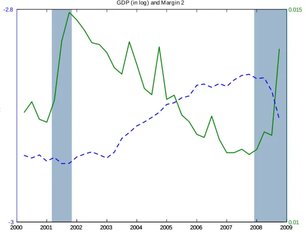
During the two most recent recessions of 2001 and 2007–2009, the net interest margins of banks in the United States rose by approximately 20in under a year, whereas they steadily
Corresponding author: Université Paris-Dauphine, LEDA-SDFi. Place du Maréchal de Lattre de Tassigny. 75775 Paris Cedex 16, France. Tel. (+33)1 4405 4719. Email: kevin.beaubrun@dauphine.fr.
declined during the expansion of 2002–2006.1 These …gures illustrate the countercyclical behaviour of the net interest margin2, which is of considerable importance given the
impact of interest rates on the pro…tability of banks, on macroeconomic activity, and on monetary policy.3 We herein provide a new theoretical explanation of this behaviour by
investigating the possible e¤ects of search frictions on the credit market.
Recent studies have used a search framework to explain the consequences of imper-fections on the credit market in line with the approaches proposed by Den Haan et al. (2003) and Wasmer and Weil (2004). The premise of the research e¤orts of these authors is that new credit arrangements are not instantaneous, but are rather costly and time consuming. These constraints are mainly due to imperfect access to the information of agents. As a result, agents must spent time and resources meeting their counterpart’s needs (e.g., …nding a loan for entrepreneurs or …nding an entrepreneur for banks).4 A
key point in this literature is the powerful nature of the ampli…cation and propagation mechanisms associated with matching friction on the credit market. While many authors have provided detailed analyses of the equilibrium amount of credit market quantities, they have not studied the dynamics of credit market prices, namely the interest rates and margins that ensue.5 This paper therefore contributes to the body of knowledge on credit
market search by demonstrating the relevance of such a mechanism in accounting for the countercyclical behaviour of the net interest margin.
The model developed herein is in the spirit of the matching models presented by Diamond (1982), Mortensen and Pissarides (1994), and Pissarides (2000).6 The model
proposed herein incorporates the following three components: (i) an aggregate matching function that identi…es the search-and-meet processes and then determines the ‡ow of new matches as a function of the mass of unmatched entrepreneurs and the searching intensity of lenders; (ii) a …nancial contract that determines the credit interest rate as an outcome of a Nash bargaining solution; and (iii) an endogenous separation process, which is the consequence of idiosyncratic shocks on the entrepreneur’s technology production.7 By
qualitatively analysing the model’s equilibrium, we thus derive the theoretical conditions under which the net interest margin behaves countercyclically. Based on this analysis,
our main theoretical result shows that the net interest margin’s response to technological shocks is ambiguous because of the combination of the three antagonistic e¤ects described brie‡y below.
Lenders and borrowers bargain to share the value of the match, which depends on the pro…ts yielded by the production activity. As a positive improvement in the technological shock increases the returns on the production activity and therefore the associated pro…t, the lender can then negotiate a higher loan rate. This …rst e¤ect widens the net interest margin during an expansion, but the in‡uence of such widening may be outweighed by the other two e¤ects. The second e¤ect is related to the countercyclical behaviour of the separation rate.8 During an expansion, lenders and borrowers are less selective and
accept matches that have a lower level of idiosyncratic productivity. As a result, average idiosyncratic productivity declines, the pro…ts from the production activity decrease, and the net interest margin tightens. The third e¤ect is a consequence of modi…cations to the external opportunities of entrepreneurs. For each agent, the ease of …nding another partner determines its threat point and thus its raised revenues. A positive technological shock increases the expected value of future matches, which stimulates the supply of loans on the credit market. The relative abundance of liquidity9 shortens the average delay
in …nding a loan and thus reinforces the entrepreneur’s threat point in the bargaining process. This phenomenon lowers the loan interest rate bargained by entrepreneurs and thus decreases the net interest margin. These qualitative results allow us to clarify the mechanisms at work and can be illustrated by carrying out a numerical analysis of the model. We propose a calibration of the model such that both the net interest margin and the separation rate are countercyclical and accompanied by persistent ‡uctuations in output.
The remainder of this article is organised as follows. In Section II, we present the stylised facts of interest and describe the empirical data used. The model economy is described in Section III. The equilibrium of the model is de…ned and studied in both an analytical and a numerical fashion in Section IV. A discussion of the theoretical literature is provided in Section II. Section VI concludes.
II
Some Statistics on the Net Interest Margin in
the US
In this section, we describe the cyclical behaviour of a bank’s net interest margin. In line with Alliaga-Diaz and Olivero (2011) and Corbae and D’Erasmo (2013), we focus on US commercial banks and derive our data from the Consolidated Report of Condition and Income, which is available for all banks regulated by the Federal Reserve System, the Federal Deposit Insurance Corporation, and the Comptroller of the Currency. From this report, we compile a quarterly dataset that runs from 1985 to 2008.10 Moreover, we
follow the approaches put forward by Kashyap and Stein (2000), Alliaga-Diaz and Olivero (2011), and Corbae and D’Erasmo (2013) by constructing consistent time series for our variables of interest. In the Data Appendix, we describe these variables and the data sources.
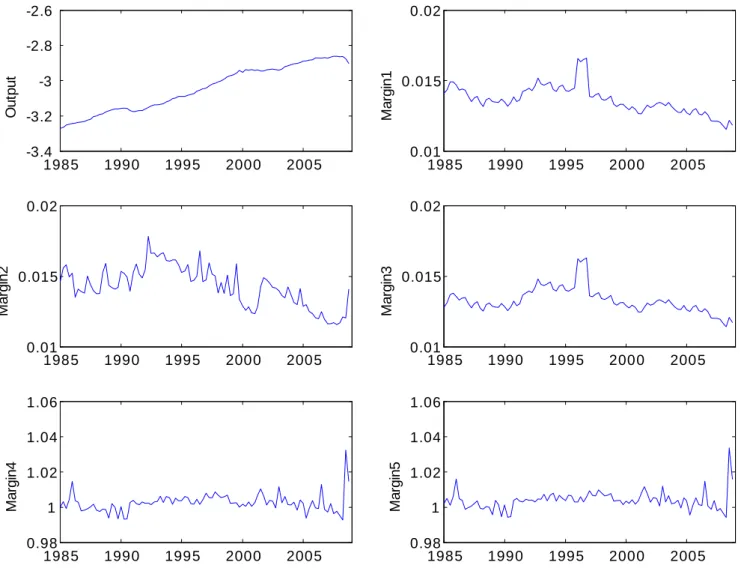
We use six de…nitions for our margins. Margins 1, 2, and 3 are all calculated as the di¤erence between (i) the ratio of interest income on loans to the volume of loans and (ii) the ratio of interest expenses on deposits to the volume of deposits. As stated in Alliaga-Diaz and Olivero (2011), the main di¤erence among these de…nitions is the way in which loan volume is adjusted for delinquent loans.11 Margins 4 and 5, derived from the FRED Database, are de…ned as the net interest margin for all US banks and the net interest margin for all US banks that have average assets under one billion dollars, respectively. Margin 6 is the only case in which macrodata used the spread between the bank prime and the three-month Treasury bill rates. As pointed out by Alliaga-Diaz and Olivero (2011) and Dueker and Thornton (1997), a change in the prime rate is indicative of a general shift in lending rates.
The historical series are shown in Figure 3 in the Appendix together with our proposed measure of the business cycle, namely real GDP per capita. The net interest margin series show substantial di¤erences according to the de…nition of average values, volatilities, and historical evolution. This …nding shows the importance of using di¤erent measures of the net interest margin to present robust empirical facts. To provide an insight into
the countercyclical behaviour of the net interest margin, we also extract the cyclical components of GDP per capita and the net interest margin for the entire sample period.
"Table 1 here"
Table 1 presents the contemporaneous correlations with GDP, while Figure 4 illustrates the correlations at lead and lags (k = 4to k = 4) with the associated con…dence interval. Despite clear di¤erences in the series, they all show signi…cant countercyclical behaviour. The correlation coe¢ cient ranges between -0.26 and -0.48 and is always nonzero at the 1% level (except for Margin 3 whose correlation with output is only nonzero at the 5% level). Moreover, a signi…cant negative correlation is still observed if we consider one lead or one lag for the margin. These values are consistent with the evidence presented by Aliaga-Diaz and Olivero (2011) and Corbae and D’Erasmo (2013).
III
The Model Economy
Let us assume that the model economy is populated by two types of agents: entrepreneurs and …nancial intermediaries (lenders). Entrepreneurs specialise in project management and produce a unique …nal good. Our model assumes that entrepreneurs have no private wealth and use the lender’s funds as the sole productive input. This assumption implies that production feasibility depends on the availability of the funds provided by lenders. In the same vein, the …nancial intermediary (or bank) is endowed with funds but has no skill to manage production projects.
Since the credit market is subject to search frictions, banks must pay a …xed search cost to …nd an entrepreneur on the market in a given period. A bank is only allowed to allocate its funds to an entrepreneur with whom it is currently matched. The bank must therefore form a bilateral long-term relationship with an entrepreneur. Once a lender– entrepreneur pair has been formed, a …nancial contract is agreed between these agents that determines the price of the funds lent by the bank.
The …nal good technology is subject to both an aggregate productivity shock and an idiosyncratic productivity shock. The amount of production, and thus the entrepreneur’s
ability to repay a debt, is therefore related to both these productivity levels. If the idiosyncratic productivity level is su¢ ciently high, then contracting in a given period will be solved according to a Nash bargaining solution. If not, both parties will agree to sever the relationship in order to avoid paying the …xed costs of production and loan management, and both agents will return to the credit market.
The following three subsections describe the model’s key mechanisms in more detail: (i) the matching function and search behaviours, (ii) idiosyncratic productivity shocks and the choice of the reservation productivity threshold, and (iii) the …nancial contract that determines the credit interest rate as an outcome of a Nash bargaining solution.
1
The Matching Process
Let E be the population of entrepreneurs and let Nt represent the number of
entrepre-neurs matched with lenders. The ‡ow of new matches Mt is a function of the numbers of
unmatched entrepreneurs, (E Nt)and the lenders’loan supply, Vt. The search friction
is summarised by an increasing and concave matching function Mt = m (Vt; E Nt) <
minfVt; Et Ntg. The assumption of constant returns to scale for the matching
technol-ogy leads to the following properties for matching probabilities: (1) qt= q ( t) = p ( t) t = pt t :
Here, qt = Mt=Vt is the lender’s matching probability, whereas pt = Mt= (E Nt) is the
matching probability for entrepreneurs. Importantly, t= Vt= (E Nt) represents credit
market tightness. As Vt increases, the tightness of the market also increases. t could
be interpreted as a liquidity index: in this context, the more lenders supply loans, the more liquid the market.12 In the remainder of this subsection, we assume a standard
Cobb–Douglas matching function, with a scale parameter m > 0 and elasticity parameter 0 < < 1. Consequently, the matching probability for entrepreneurs is
We de…ne the law of motion of the rate of matched entrepreneurs, nt = Nt=E, as
follows:
(3) nt+1= (1 st+1) [nt+ m (vt; 1 nt)] ;
where vt = Vt=E and st represent the endogenous rate of separation per period. The
separation rate concerns both old matches, nt, and new matches, mt.
2
Idiosyncratic Productivity Shocks and Reservation
Produc-tivity
Entrepreneurs are expected to undertake projects to produce yt units of the …nal good
(the numeraire) according to the following constant returns to scale technology: yt(!) = zt!,
where ztis the aggregate productivity level and ! the idiosyncratic productivity level.
The …xed amount of the loan is normalised to unity, without loss of generality. In each period, all entrepreneurs pick a new value for ! from the uniform distribution function G (!) that satis…es dG (!) =d! = 1= (! !) ; with ! > !. ! is assumed to be perfectly observed by lenders.
Let Jt(!) be the entrepreneur’s value function of being matched with an idiosyncratic
productivity level !. We have Jt(!) = maxfJta(!) ; Vteg, where the entrepreneur that
accepts the match obtains the value function Jta(!). Otherwise, he or she turns to the
credit market and then has the value function Ve
t: Reservation productivity is de…ned as
the level e!et that satis…es the condition Ja t (!e e t) = Vte: (4) maxfJta(!) ; Vteg = 8 > < > : Ja t (!) ; ! !e e t Vte; ! <!eet
t(!), the value function for matched lenders, also depends on the idiosyncratic
to the realised value of !, a lender decides either to accept the match, in which case it obtains the value function a
t (!), or to refuse it, thereby obtaining Vtb. For lenders, the
reservation productivity level !ebt satis…es the condition a t !e b t = Vtb, with (5) max at (!) ; Vtb = 8 > < > : a t (!t) ; ! !ebt Vb t; ! <!e b t
Depending on the productivity of the project, matched lenders and entrepreneurs will decide either to pursue or to sever the credit relationship. If they choose to maintain coop-eration, they will negotiate a …nancial contract in which a loan interest rate is determined.
3
The Financial Agreement
The …nancial contract determines the loan interest rate, R`t(!), as a function of !, the
idio-syncratic productivity of the entrepreneur’s technology. The interest rate is the outcome of a Nash bargaining solution, where the respective bargaining power of the entrepreneur and lender are represented by and (1 ). The use of this Nash bargaining solution leads to the traditional sharing rule:
(6) at(!) Vtb = (1 ) (Jta(!) Vte)
The outcome of the bargaining process ensures equality between the reservation pro-ductivity of the lender and that of the entrepreneur: !et = e!et =!e
b
t. Indeed, the sharing
rule (6) implies that the entrepreneur’s payo¤ (Ja
t (!) Vte) is the share (1= 1) 1
of the lender’s payo¤ a
t(!) Vtb . Therefore, for any !, if the lender wishes to pursue the
relationship (which requires at (!) to be greater than or equal to Vtb), this implies that
the entrepreneur will also wish to stay matched. Therefore, the condition Jta(!) > Vte
must hold for entrepreneurs as well, and …nally reservation productivity e!t must satisfy
(7) Jta(!et) Vte= 1
a
For this value of reservation productivity !et, the separation rate is de…ned as (8) st = Z !et ! dG (!) = !et ! ! ! given the uniform distribution of !.
IV
Equilibrium Credit Cycle Properties
This section discusses the credit cycle properties of the model presented in Section III. We …rst describe the theoretical properties and then use a numerical analysis to demon-strate the model’s ability to reproduce the stylised facts. The full resolution of the model is presented in the Appendix. Subsection B de…nes the value functions introduced in the previous section, while Subsection C details the calculus for the equilibrium decisions concerning the entry, separation, and bargaining. Finally, the full equilibrium character-isation (de…nition, existence, and stability) is developed in Subsection D.
1
Theoretical Results
The topic of interest here is the cyclical characterisation of the net interest margin fol-lowing a technological shock. Therefore, in the present paper, we de…ne the equilibrium net interest margin to be the di¤erence between the rate of return on a loan, Rt`(!), and
the cost of the resources for the lender, Rh. To account for the heterogeneity of matches,
the net interest margin is de…ned to be the average of the individual margins:13
(9) Rpt = (1 ) zt
(! +!et)
2 x
e Rh + xb d
t
Equation (9) is the weighted average of two terms whose coe¢ cients represent the re-spective bargaining power of the agents (1 ) and . For = 1, which corresponds to the extreme case of the absence of bargaining power for the lender. The credit spread depends on two variables, namely the lender’s cost, xb, and credit market tightness,
t. In
the entire surplus from the production process, i.e., the average value of the production carried out by entrepreneurs, zt(! +e!t) =2, less the …xed cost of production, xe, and less
the interest paid to depositors, Rh.
The business cycle behaviour of an endogenous variable is characterised by its elasticity with respect to the technological shock, denoted z; which satis…es bt = zbzt, where
bt = log ( t= ) is the logdeviation of the variable t, for = fRp; ;!eg, and bzt the
logdeviation of the productivity shock. Based on this de…nition, the elasticity of the net interest margin with respect to the technological shock (see equation (D.14) in Appendix D) is (10) RpRpz = (1 ) ! +!e 2 z + (1 ) e ! 2z!ez d z
We now describe the conditions under which the net interest margin may behave countercyclically by analysing the sign of Rp
z. As shown by (10), the elasticity of the net
interest margin to the technological shock is a function of the elasticities of credit market tightness, z, and of reservation productivity, !ez . Therefore, we must …rst illustrate the
link between the credit market tightness and the technological shock. We can then repeat the same exercise with reservation productivity.
Proposition 1 Credit market tightness is procyclical.
Proof. The elasticity of the credit market tightness to a technological shock (see equa-tion (D.12) in Appendix D) is (11) z = z 1 ! +e! ! !e 1 2 d z (! e!) 1 m 1 z 1
where z is unambiguously positive, z > 0, given the stability condition demonstrated in
the proof of Proposition 5 (see Appendix D).
Credit market tightness responds positively to productivity shocks. Following a pos-itive aggregate technological shock, lenders are willing to increase their search e¤orts on the credit market. Indeed, improvement in the entrepreneurs’technology signals higher
productivity for the following periods.14 This mechanism is therefore clearly related to the persistent nature of shocks. The more persistent the productivity shock, the more positive is the credit market tightness. With no persistence, z = 0, and the credit market tightness would become unambiguously acyclical.
Proposition 2 The separation rate is countercyclical if (12) (1 )
This is a su¢ cient (and not necessary) condition for a negative elasticity of the separation rate to a technological shock, namely !ez < 0.
Proof. The expression for the elasticity of reservation productivity to a technological shock is e !z = 1 m 1 (1 ) d z!e z 1
as shown in equation (D.13) in Appendix D. Moreover, the case of !ez < 0 requires
1 m 1
(1 ) d
ze! z < 1
since z > 0, a su¢ cient but not necessary condition of !ez < 0 is
1 m > 1
which is necessarily satis…ed under condition (12), because m is the entrepreneur’s matching probability and therefore below unity.
This condition (12) is always satis…ed if the Hosios (1990) condition of e¢ ciency holds, namely = (1 ). In this case, the trading externalities of the matching function are internalised in the Nash bargaining process given that the equilibrium reservation productivity depends on the technological shock via two mechanisms.
idio-syncratic productivity. In other words, a 1aggregate productivity leads to a 1productivity, because the separation is based on the overall level of the entrepreneur’s productivity.15
The second mechanism by which a technological shock a¤ects reservation productivity arises from the response to credit market tightness, which in turn a¤ects reservation productivity !et in two ways.
Firstly, the free entry condition states that the expected value of a match for lenders is equal to the average cost of a match: the higher the value of t, the higher the value of
a match. In this case, lenders and entrepreneurs accept lower idiosyncratic productivity in order to preserve their current matches and, as a result, !et decreases with t.16
Secondly, as credit market tightness increases, better external opportunities emerge for entrepreneurs, who are therefore able to bargain lower interest rates from their partners. This bargaining process provokes a decline in the equilibrium bargained loan interest rate. In this way, high values of tmake lenders more selective and thereby increase the required
reservation productivity level. In such a case, !et increases with t.17
From here, we assume that condition (12) is satis…ed and we therefore examine the conditions of the countercyclical behaviour of the net interest margin.
Proposition 3 The net interest margin is countercyclical if (13) (1 ) ! +!e
2 z < d z+ (1 ) e !
2z ( !ez)
Under this condition, the elasticity of the net interest margin to a technological shock is negative, namely Rpz < 0.
Proof. This condition is deduced from the de…nition of Rpz in equation (10) and
Propositions 1 and 2.
The elasticity of the net interest margin to a technological shock, Rpz, allows us to
assess whether this variable behaves countercyclically. The sign of Rpz depends on three
components, each related to one of the following coe¢ cients: z; !ez, or z (see Equation
(10)).
shock increases pro…ts for the entrepreneur through a technological improvement (the coe¢ cient of z in Equation (10)). As the bargaining power of lender (1 ) is higher, he or she may wish to take advantage of this in order to negotiate a higher loan interest rate. The size of this …rst e¤ect thus depends on the lender’s bargaining power and the average productivity of matches, namely (! +!) z=2. The greater the bargaining powere of the lender, the greater the appropriation of pro…t and the higher the impact of the technological shock on the net interest margin.
The second e¤ect generates a countercyclical net interest margin related to the average productivity of matches (the coe¢ cient of !ez in (10)). As reservation productivity !et
drops in response to a positive shock, the average productivity of matches reduces. The consequences for pro…ts are the opposite of those of the …rst e¤ect, leading therefore to a decrease in the net interest margin.
The third e¤ect serves to generate a countercyclical net interest margin similar to the second. This e¤ect is based on the threat point of entrepreneurs, which is in‡uenced by credit market liquidity (the coe¢ cient of z in (10)). To understand which mechanism
is at work, note that d = p (d=q), which implies that an entrepreneur can …nd another match, with a probability p, and obtain a share of the value of that match, d=q. Consequently, as the credit market tightens following a positive shock, better external opportunities present themselves to entrepreneurs, which signi…cantly increases their threat point and tightens the net interest margin further.
To conclude, the second and third e¤ects (the RHS term of (13)) must be su¢ ciently large to outweigh the …rst term (the LHS term of (13)) in order for the net interest margin to behave countercyclically. However, because the previous analysis of the equilibrium does not allow us to draw unambiguous conclusions about the model’s ability to foster a countercyclical net interest margin, we now numerically simulate the model’s solution in order to assess the plausibility of the presented theoretical model.
2
Numerical Analysis
The previous theoretical analysis emphasised the interactions between the several mech-anisms that determine the behaviour of the net interest margin. Some of the e¤ects of a technological shock induce a procyclical net interest margin dynamic, whereas others lead to countercyclical behaviour. In what follows, we present numerical exercises carried out in order to assess and quantify the relative importance of these mechanisms according to the values of the structural parameters used in the present study.
2.1 Calibration
First, the model is calibrated by choosing the available empirical counterparts for the variables of interest. Because none of the previous variables allows us to calibrate all the structural parameters, we make additional assumptions about the values of these parameters.
We restrict their ranges using the conditions of the existence, uniqueness, and stability of the equilibrium. The unit of time is taken to be one quarter. The calibration constraints on interest rates are as follows. For our sample data, the quarterly interest rate on lender resources is Rh = 1:02041=4 and the quarterly interest rate on loans is R` = 1:03921=4. Further, transition probabilities are …xed at the following values: p = 0:5; q = 0:75, and s = 1=16: On average, it takes two quarters for an entrepreneur to …nd a lender and the lending relationship lasts four years. The condition of Hosios (1990) is imposed, namely = = 0:5, and the scale parameters of the production and matching technologies are then set as follows: ! = 0:90; ! = 1; and z = 4. Finally, the discount rate is set to a conventional value = 0:995. We then deduce from the steady-state restrictions the values of!; ; m; d; xe e; xb; n;and Y . In the following subsection, we describe the business
cycle behaviour of the model for this calibration.
2.2 The Cyclical Behaviour of the Net Interest Margin
We start the numerical analysis by describing the dynamic behaviour of the aggregate variables. Figure 5 depicts the impulse response functions (IRFs) to a positive
technolog-ical shock on output, the net interest margin, and reservation productivity. As shown in Proposition 3, the shock’s persistence plays a crucial role in the cyclical behaviour of the net interest margin. Therefore, the model is simulated for the two alternative values of
z =f0:35; 0:95g :
In both these cases, a positive technological shock leads to an expansion of the credit in the economy by two means. Firstly, an improvement in aggregate technology leads to lenders and entrepreneurs accepting a lower idiosyncratic productivity level. Because our calibration respects condition (12), the elasticity coe¢ cient !z is negative and the IRF
of !et is negative in both cases. This fall in reservation productivity decreases the rate of
match destruction in the economy and leads to a credit expansion.
Secondly, the improvement in aggregate technology stimulates the entry of lenders into the credit market. In Proposition 1, we showed that the elasticity z > 0 and thus
the IRF of t is positive. This rise in credit market tightness facilitates the …nancing of
entrepreneurs by increasing their matching probabilities and thus contributes to a credit expansion. However, the magnitude of the response of credit market tightness depends crucially on the shock’s persistence because of the forward-looking behaviour of agents. In the case of low persistence, the increase in credit market tightness is moderate with important consequences for output and the net interest margin, as discussed below.
For output, the IRFs are positive for both values of z. However, the hump-shaped pattern, as emphasised by Den Haan et al. (2003), is no longer observed for moderately persistent shocks. For the net interest margin, the sign of its IRFs is related to the shock’s persistence. When persistence is high, the net interest margin reacts negatively to the shock, leading to a negative correlation with output (approximately 0:99). This result is consistent with the observed countercyclical behaviour of the net interest margin in the United States, as described in Section II. If low persistence is assumed, the model loses its ability and generates a procyclical net interest margin. The small response of credit market liquidity reduces the threat point e¤ect drastically. Therefore, entrepreneurs do not bene…t from a signi…cant improvement in liquidity and are thus unable to bargain a lower interest rate.
2.3 Robustness
In order to assess the robustness of the numerical results to the speci…c values selected in the calibration process, Figure 6 reports the coe¢ cient of correlation between the net interest margin and output for various structural parameters and calibrated endogenous variables. The ranges of values used are selected to satisfy the conditions of equilibrium existence and stability given in Appendix D.
When the value of a calibrated endogenous variable is changed, the overall calibration process described above is applied and we adapt the values of the structural parameters as necessary. The net interest margin becomes procyclical when (i) low persistent shocks are considered (as shown in the previous subsection) and (ii) a high separation rate is imposed (for values above 40%, which implies a …nancial relationship that lasts for less than 2.5 quarters).
V
Relations with the Theoretical Literature
The presented explanation of the cyclical behaviour of the net interest margin based on search frictions is not the …rst proposed in the literature. Business cycle models with …nancial frictions have been widely based on costly state veri…cation theory, as …rst suggested by Townsend (1979) and later incorporated into business cycle models by Bernanke and Gertler (1989). The countercyclical behaviour of the net interest margin in this context should result from the countercyclicality of default rates. In times of economic recession, borrowers receive less compared with the value of their collateral than they do in better economic times. Further, the probability of borrowers defaulting on their loans increases in recessions and this forces banks to increase their lending rates compared with the costs of their deposits.
Carlstrom and Fuerst (1997), Gomes et al. (2003), and Covas and Den Haan (2012) all demonstrated the di¢ culty of this framework generating a countercyclical default rate and suggested extensions to overcome this problem. In addition, Bernanke et al. (1999) made the seminal …nding that costly state veri…cation theory is a convenient ampli…cation
mechanism of shock e¤ects, but not per see a powerful propagation mechanism. The purpose of the credit market search model is thus both to generate persistent ‡uctuations, as demonstrated by Den Haan et al. (2003), and a countercyclical separation rate, as shown in the present paper.
The second set of explanations is linked to the macroeconomic literature on coun-tercyclical mark-ups in markets associated with imperfect competition (e.g., Rotemberg and Woodford, 1992). One representation of this approach was proposed by Olivero (2010), who introduced a monopolistically competitive banking sector into a standard two-country, two-good business cycle model with complete asset markets. The counter-cyclical margin in the model presented by Olivero (2010) rested on the counter-cyclical variations in the number of banks and in their di¤erentiation. Corbae and D’Erasmo (2013) also focused on imperfect competition in the context of a model of banking industry dynamics based on Stackelberg monopolistic competition. This approach aimed to provide a full treatment of the bank, in particular its endogenous size. Therefore, it would be interest-ing to adopt this approach for the credit market search model.18 Indeed, in the literature as in this paper, …nancial intermediation activities are linear, while bank size has no consequences on the credit market.
Recently, Aliaga-Diaz and Olivero (2012) o¤ered another explanation of net interest margin dynamics based on deep habits. Interestingly, their explanation shares a key assumption with the credit market search model, namely the existence of switching costs. These authors introduced deep habits as a way of modelling switching costs, which are similar to the search costs considered in the present paper. Switching costs correspond to the search costs that agents must repay after separation in order to form a new match.
VI
Conclusion
This paper formulated a credit market search model that reproduces the well known coun-tercyclical behaviour in the net interest margins of banks. Our contribution to the body of knowledge in this regard is to demonstrate that the relevance of the credit market search model is not restricted to "quantities" (e.g., credit, output, or unemployment),
but can also be applied to "prices" (e.g., interest rates). Credit market liquidity, mea-sured by credit market tightness, plays a crucial role in our model because it determines the countercyclical behaviour of the net interest margin. As credit market tightness is time-varying, this model’s property is in line with the research directions suggested by Petrosky-Nadeau and Wasmer (2013) . Although time-invariant in their model19, these
authors clearly stated that time-varying credit market tightness is an attractive mecha-nism for overcoming …nancial issues. Finally, the presented setup explains the procyclical behaviour of liquidity on the credit market as well as the countercyclical behaviour of the net interest margin and separation rate, consistent with persistence in output ‡uctuations.
VII
ACKNOWLEDGEMENTS
This paper bene…ted from the comments and suggestions of Hafedh Bouakez, Jerôme de Boyer des Roches, Dean Corbae, Pablo d’Erasmo, Nicolas Petrosky-Nadeau, and Etienne Wasmer as well as the seminar participants of the GDR Monnaie et Finance (Orléans, 2009), the Annual Meeting of the SED (Montréal, 2010), the Louis Bachelier Institute Seminar (Paris, 2010), the Annual Meeting of T2M (2010, Le Mans), the MSE Université Paris I Seminar (2009), and the Université de Nantes (2010). The authors also thank Samir Ifoulou for research assistance. Fabien Tripier gratefully acknowledges the …nancial support provided by the Chair Finance of the University of Nantes Research Foundation. Kevin Beaubrun-Diant gratefully acknowledges the …nancial support received from the Dauphine Research Foundation.
Notes
1The net interest margin is calculated as the di¤erence between (i) the ratio of interest income on
loans to the volume of loans and (ii) the ratio of interest income on deposits to the volume of deposits. The exact values reported in Figure 1 are 1.23% in 2001(1), 1.49% in 2001(4), 1.16% in 2007(4), and 1.41% in 2008(4). Figure 2 shows the cyclical components of these two series for the period 1985–2008.
2Although this empirical fact is not entirely new, the full empirical analysis has only recently been
provided by Aliaga-Diaz and Olivero (2010, 2011) and Olivero (2010). In the present paper, we closely follow the empirical approach of Aliaga-Diaz and Olivero (2010), as discussed in more detail in Section II on the empirical literature. In this section, we also describe our data and compute the correlation coe¢ cients between the net interest margin and output for a longer time period and for various measures of the margin compared with the literature on this topic.
3A large body of knowledge on the structural determinants of the net interest margin aims to explain
international di¤erences in banking pro…tability as well as recent trends in this sector. For instance, Ho and Sanders (1981) and Wong (1997) developed the theoretical foundations of this topic, while Demirgüç-Kunt and Huizinga (1999) exempli…ed previous empirical works. For the macroeconomic implications of this research stream, see Tobias and Shin’s (2010) work on …nancial intermediaries. These authors showed that the net interest margin in‡uences monetary policy by determining the pro…tability of bank lending, and thus the capacity of banks to increase lending in the economy.
4Dell’Ariccia and Garibaldi (2005) and Craig and Haubrich (2013) both constructed databases of credit
‡ows and showed that the US credit market is characterised by large cyclical ‡ows of credit expansions and contractions that can be explained in terms of matching friction.
5The important macroeconomic consequences of credit market quantities were put forward by Den
Haan et al. (2003) for output dynamics and by Wasmer and Weil (2004) and Petrosky-Nadeau and Wasmer (2013) for equilibrium unemployment. Wasmer and Weil (2004) and Besci et al. (2005) also examined equilibrium interest rates in the credit matching model, but only at the steady state and not for the business cycle as addressed in the present study.
6This basic structure of the credit matching model (i.e., an aggregate matching function and a Nash
bargaining process for interest rates) was used by Wasmer and Weil (2004) and Petrosky-Nadeau and Wasmer (2013) in association with search frictions on the labour market, by Besci et al. (2005) with heterogeneous borrowers, by Petrosky-Nadeau and Wasmer (2011) in a model of search frictions on three markets (labour, credit, and goods), and by Rochon and Chamley (2011) for loan rollovers. Note that Den Haan et al. (2003) did not consider the Nash solution for the interest rate, but instead explored an agency contract with moral hazard. Liquidity shocks for lenders were also considered.
7The inclusion of the third component is necessary to generate a countercyclical net interest margin
in the credit market search model. By contrast, an exogenous separation process would lead to the net interest margin being procyclical.
8The countercyclical behaviour of the default rate is a well established empirical fact (see Gomes et al.
(2003) and Covas and Den Haan (2012) for the implications on the business cycle). In our model, such a separation is based on a joint decision by the lender and the borrower and cannot therefore strictly be interpreted as a default even though the two events (i.e., failure and separation) lead to the entrepreneur
losing his or her long-term lending relationship with the bank.
9Here, we use the term "liquidity" to express the "ease and speed" experienced by an entrepreneur
when his or her status switches from "un…nanced" to "…nanced".
10Our study period ends in 2008 in order to avoid the period of the global …nancial crisis. Since
then, monetary policy has become unconventional, which could have modi…ed net interest margin behaviour signi…cantly. Although this topic is of clear research interest, it is beyond the scope the present paper.
11Corbae and D’Erasmo (2012) considered only Margin 3.
12Using the terms introduced in footnote I, the credit market is more liquid when rises in the sense
that entrepreneurs …nd "easier" and more "speedy" lenders thanks to a higher matching probability, de…ned as p = m .
13This equation is deduced by introducing into Rp t = R! e !t R ` t(!) Rht dH (!) the expression of R`t(!) given by (C.3).
14See equation (D.1), where the expected productivity for tomorrow, that is E
tfzt+1g, determines the
current credit market liquidity, t.
15See the LHS term of equation (D.2), which determines reservation productivity. 16This corresponds to (d=m) 1
t in the RHS term of equation (D.2), which determines reservation
productivity.
17This corresponds to ( m
t) in the RHS term of equation (D.2), which determines reservation
productivity. See equation (C.3) for the impact of this term on the bargained loan interest rate.
18In the labour market search literature, a speci…c strand has demonstrated the interest of considering
large …rms with nonlinearities in their production or search activities (see Bertola and Caballero, 1994).
19Credit market tightness is assumed to be acyclical by Petrosky-Nadeau and Wasmer (2013) because
there is a double free entry condition for entrepreneurs and banks. Petrosky-Nadeau and Wasmer (2013) considered endogenous (exogenous) participation for banks and entrepreneurs (workers), as in the seminal paper by Wasmer and Weil (2004). Because we only consider a unique frictional market, participation is endogenous on only one side of the market (here banks as well as …rms in the labour market search model) and exogenous on the other (here entrepreneurs as well as workers in the labour market search model).
REFERENCES
ADRIAN, T., SHIN, H.S., 2010. Financial Intermediaries and Monetary Economics, Chapter 12 in Handbook of Monetary Economics, Volume 3, edited by B. M. Friedman and M. Woodford, 601–650.
ALIAGA-DIAZ, Roger A. and OLIVERO, Maria P. “The Cyclicality of Price-Cost Mar-gins in Credit Markets: Evidence from US Banks” ECONOMIC INQUIRY 49.1 (Jan 2011):26-46
ALIAGA-DIAZ, Roger A. and OLIVERO, Maria P. “Is there a Financial Accelerator in US Banking? Evidence from the Cyclicality of Banks’Price-Cost Margins”ECONOMICS LETTERS 108.2 (Aug 2010):167-171
BECSI, Z., LI., V.E. and WANG, P. (2005). Heterogeneous borrowers, liquidity, and the search for credit. Journal of Economic Dynamics and Control. 29 (8), 1331-1360.
BERNANKE, B. S. and GERTLER, M. (1989). Agency costs, net worth, and business ‡uctuations. American Economic Review, 79 (1), 14-31.
BERTOLA, G., and CABALLERO, R. J. (1994). Cross-sectional e¢ ciency and labour hoarding in a matching model of unemployment. The Review of Economic Studies, 61(3), 435-456.
CHAMLEY, C. and ROCHON, C. (2011). From search to match: when loan contracts are too long. Journal of Money, Credit and Banking, 43, 385-411.
CORBAE, D. and D’Erasmo, P. (2011). A quantitative model of banking industry dy-namics. Working paper.
COVAS, F. and DENHAAN, W.J., (2012). The Role of Debt and Equity Finance Over the Business Cycle. The Economic Journal vol. 122, Iss. 565, 1262-1286.
CRAIG, B.R. and HAUBRICH, J.G. (2013). Gross loan ‡ows. Journal of Money, Credit and Banking 45 (2-3), 401–421.
DELL’ARICCIA, G. and GARIBALDI, P. (2005). Gross credit ‡ows. Review of Eco-nomic Studies 72 (3), 665-685.
DEMIRGUC-KUNT, A., and H. HUIZINGA (1999). Determinants of Commercial Bank Interest Margins and Pro…tability: Some International Evidence, World Bank Economic
Review 13(2), 279-408.
DEN HAAN, W.J., RAMEY, G. and WATSON, J. (2003). Liquidity ‡ows and fragility of business enterprises. Journal of Monetary Economics 50 (6), 1215-1241.
DIAMOND, P. A. (1982), Wage determination and e¢ ciency in search equilibrium. Re-view of Economic Studies, 49, 217-27.
GOMES, J., A. YARON and L. ZHANG, 2003, Asset Pricing and Business Cycles with Costly External Finance", Review of Economic Dynamics, vol. 6, 767-788.
HO, T., and A. SAUNDERS, 1981. The determinants of bank interest margins: theory and empirical evidence. Journal of Financial and Quantitative Analyses 16, 581–600. IACOVIELLO, M. (2011). Financial business cycles. Federal Reserve Board.
KOLLMANN, R. (2012). Global banks, …nancial shocks and international business cycles: Evidence from estimated models. Working Papers ECARES ECARES.
MORTENSEN, D.T. and PISSARIDES, C.A. (1994). Job creation and job destruction in the theory of unemployment. Review of Economic Studies, 61 (3), 397-415.
OLIVERO, M.P. (2010). Market power in banking, countercyclical margins and the international transmission of business cycles. Journal of International Economics. 80 (2). 292-301.
PETROSKY-NADEAU, N. and WASMER, E. (2011). Macroeconomic dynamics in a model of goods, labor and credit market frictions. IZA Discussion Papers 5763.
PETROSKY-NADEAU, N. and WASMER, E. (2013). The Cyclical Volatility of La-bor Markets under Frictional Financial Markets American Economic Journal: Macroeco-nomics 5(1), 1–31 .
PISSARIDES, C.A. (2000). Equilibrium unemployment theory. MIT Press.
ROTEMBERG, J.J. and WOODFORD, M. (1992). Oligopolistic pricing and the e¤ects of aggregate demand on economic activity. Journal of Political Economy, 100 (6), 1153-1207. RAJAN, R.G. (1992). Insiders and outsiders: The choice between informed and arm’s length debt. Journal of Finance 47, 1367–1400.
SANTOS, J.A.C and WINTON, A. (2008). Bank loans, bonds, and information monop-olies across the business cycle. Journal of Finance, LXIII (3), 1315-59
TOBIAS, A.and SHIN, H.S. (2010). "Liquidity and leverage," Journal of Financial Inter-mediation, Elsevier, vol. 19(3), 418-437.
TOBIAS, A.and SHIN, H.S. (2010). "The Changing Nature of Financial Intermediation and the Financial Crisis of 2007–2009," Annual Review of Economics, Annual Reviews, vol. 2(1), 603-618.
TOWNSEND, R. (1979). Optimal contracts and competitive markets with costly state veri…cation. Journal of Economic Theory, 21, 265-93.
WASMER, E. and WEIL, P. (2004). The Macroeconomics of labor and credit market imperfections. American Economic Review 94 (4), 944-963.
WONG, K.P. (1997). On the determinants of bank interest margins under credit and interest rate risks. Journal of Banking and Finance 21, 251–271.
GDP (in log) and Margin 2 G DP (-) 2000 2001 2002 2003 2004 2005 2006 2007 2008 2009 -3 -2.8 2000 2001 2002 2003 2004 2005 2006 2007 2008 20090.01 0.015 M ar gi n 2( :)
Figure 1: Output and net interest margin during the two last recessions and the expansion phase of 2002-2007.
Cycl ical gdp and m argi n2 C yc lic a l g d p ( -) 1985 1990 1995 2000 2005 2010 -0.05 0 0.05 1985 1990 1995 2000 2005 2010-5 0 5 x 10⁻³ C y c lic a l marg in 2(: )
Figure 2: Cyclical components of GDP (in log) and of the net interest margin (HP Filter 1600).
Table 1. Sample Relative Volatility and Correlations with GDP
(level of signi…cance in parenthesis)
Volatility Correlation margin 1 0:0437 0:2680 (0:0083) margin 2 0:0669 0:3091 (0:0022) margin 3 0:0436 0:2477 (0:0150) margin 4 0:4184 0:4653 (0:0000) margin 5 0:4149 0:4510 (0:0000) margin 6 0:4199 0:4839 25
1985 1990 1995 2000 2005 -3.4 -3.2 -3 -2.8 -2.6 O ut put 1985 1990 1995 2000 2005 0.01 0.015 0.02 M ar gin1 1985 1990 1995 2000 2005 0.01 0.015 0.02 M ar gin2 1985 1990 1995 2000 2005 0.01 0.015 0.02 M ar gin3 1985 1990 1995 2000 2005 0.98 1 1.02 1.04 1.06 M ar gin4 1985 1990 1995 2000 2005 0.98 1 1.02 1.04 1.06 M ar gin5
-4 -2 0 2 4 -1 -0.5 0 0.5 1 corr(Output(t),X(t+k)) k M a rg in1 -4 -2 0 2 4 -1 -0.5 0 0.5 1 corr(Output(t),X(t+k)) k M a rg in2 -4 -2 0 2 4 -1 -0.5 0 0.5 1 corr(Output(t),X(t+k)) k M a rg in3 -4 -2 0 2 4 -1 -0.5 0 0.5 1 corr(Output(t),X(t+k)) k M a rg in4 -4 -2 0 2 4 -1 -0.5 0 0.5 1 corr(Output(t),X(t+k)) k M a rg in5 -4 -2 0 2 4 -1 -0.5 0 0.5 1 corr(Output(t),X(t+k)) k M a rg in6
0 5 10 15 20 0 0.5 1 1.5 2 2.5 3 1a. Output ρ z=0.95 ρz=0.35 0 5 10 15 20 -20 -15 -10 -5 0 5 10
1b. Interest Rate M argi n
0 5 10 15 20 -30 -25 -20 -15 -10 -5 0 1c. Separati on Rate 0 5 10 15 20 0 1 2 3 4 5
1d. Credit Market T ig htness
Figure 5: IRFs of endogenous variables to the technological shock with a persistence of shocks equal to = 0:95 (the lines with diamonds) and equal to = 0:35 (the lines with circles).
0.9 0.92 0.94 0.96 0.98 -0.9717 -0.9716 -0.9716 β 0.4 0.6 0.8 -0.959 -0.958 -0.957 η 0.2 0.4 0.6 -0.97 -0.965 -0.96 χ 0.5 0.6 0.7 0.8 0.9 -0.974 -0.973 -0.972 ω inf 1 1.5 2 -0.974 -0.973 -0.972 ω sup 2 4 6 8 10 -0.9716 -0.9716 -0.9716 -0.9716 z 0.2 0.4 0.6 0.8 -0.95 -0.9 -0.85 -0.8 p 0.2 0.4 0.6 -0.5 0 0.5 s 0.2 0.4 0.6 0.8 -0.5 0 0.5 rho z
Figure 6: Coe¢ cient of correlation between the net interest margin and output for various values of structural parameters and of calibrated endogenous variables.
Appendix
A
Data Appendix
We focus on individual commercial banks in the U.S. The dataset compiled data from 1985 to 2008. Time series were constructed taking into account "Notes on forming consistent time series" provided by the Call Reports on Condition and Income data (available in the Federal Reserve Bank of Chicago website). We also follow Kashyap and Stein (1997), Corbae and D’Erasmo (2013) and Aliaga-Diaz and Olivero (2011).
Firstly, data was cleaned to avoid the result to be a¤ected by outlier and other obvious data problems: data for which total assets or total loans are zero or missing were deleted. Then, banks in US territories were dropped from the database.
Secondly, banks interest income, expenses are all measured as cumulative year to date totals. So we apply the appropriate adjustment to get the corresponding values for each quarter. As a result, banks for which there is no date in at least one of the four quarter, in a given year, were not included in the computation of the net of the net interest margin of that year.
Finally, we keep some de…nitions that are based on individual bank level (See Table A.1), from Aliaga-Diaz and Olivero (2011) and from Corbae and D’Erasmo (2013). When computing individual net interest margins we restrict our sample to the interval of …ve standard de…nition from the mean to control the e¤ect of outliers. We also put in the analysis of the net interest margin two time series available on the FRED database. To de‡ate balance sheets and income statements variables we use the CPI index. Variables are detrended using the HP …lter.
Table A.1. Variables De…nitions Variable Description
margin 1 Int. income on loans/loans net of loans past 90 days due int. expense on deposit/total deposits ; (riad4010/(rcfd2122 rcfd1407) riad4170/rcfd2200). margin 2 (Total int. income int. expenses)/Total loans; (riad4107 riad4073)/rcfd1400. margin 3 (Int. income from loans/Loans) (Expense from Deposits/Deposits);
riad4010/(rcfd1400 rcfd2165) riad4170/rcfd2200.
margin 4 NIMUS - The Net Interest Margin for all US banks - FRED Database. margin 5 NIM1US - The net interest margin for all US banks with average assets
under 1 billion of dollars from FRED Database.
margin 6 Bank Prime loan - Treasury Bill rate (3 months secondary market).
GDPpc Real Gross Domestic Product, 1 Decimal (GDPC1) in billions of chained 2005 US dollars. and Civilian Noninstitutional Population (CNP16OV) U.S. Department
of Labor: Bureau of Labor Statistics.
CPI Consumer Price Index - Consumer Price Index for All Urban Consumers. All Items (CPIAUCSL) Index 1982-84=100.
B
Value Functions
1
Entrepreneurs
The value functions Ja
t (!) and Vte are de…ned as follows
(B.1) Jta(!) = zt! xe R`t(!) + Et Z ! ! Jt+1(!) dGt+1(!) (B.2) Vte = pt Et Z ! ! Jt+1(!) dGt+1(!) + (1 pt) Et Vt+1e
where is the discount rate, zt! represent the value of production, R`t(!) is the credit
interests, and xe represents the …xed costs of production. We introduce …xed costs of
production to ensure the existence of a positive value for the productivity reservation !.e The probability that an entrepreneur does not …nd a lender is given by (1 pt), in which
case he must turn to the credit market in the next period. It should be noticed that being matched with a lender does not necessarily ensure that the entrepreneur is awarded funds for his project. The decision to …nance the project depends on the realized value of !.
In order to solve the bargaining process, we compute the net surplus of being matched from an entrepreneur’s perspective
Jta(!) Vte = zt! xe Rt`(!) (B.3) + (1 pt) Et Z ! ! Jt+1(!) Vt+1e dGt+1(!)
Equation (B.3) states that an entrepreneur’s net surplus is the sum of the revenue per period (total sales less production and credit costs) plus the expected value of the net surplus in the next period. The entrepreneur gets the net surplus at the new period with a probability of 1 if matched and pt if unmatched. Here, the term (1 pt) represents the
2
Banks
The value functions a
t(!) and Vtb are de…ned as follows
(B.4) at (!) = R ` t(!) R h xb+ Et Z ! ! t+1(!) dG (!) (B.5) Vtb = d + qt Et Z ! ! t+1(!) dG (!) + (1 qt) Et Vt+1b
where is the same discount rate as for entrepreneurs, R`
t(!) denotes the revenue
gen-erated by the credit activity, Rh represents the cost of the resources, xb is the …xed cost
of managing the project, d represents the per-period cost of search, and qt is the
match-ing probability for a …nancial intermediary. When matched to an entrepreneur, the net surplus of a …nancial intermediary is
a t (!) V b t = R ` t(!) R h xb+ d (B.6) + (1 qt) Et Z ! ! t+1(!) Vt+1b dG (!)
A lender’s net surplus (Equation (B.6)) is the sum of the per period income (the credit interests, minus the cost of resources, the cost of the project management, plus the search cost unpaid when matched) plus the expected value of the net surplus in the next period. The lender gets the net surplus at the new period with a probability of 1 if matched and qt if unmatched. Here, the term (1 qt) represents the di¤erence between
the matching probabilities of the two states.
C
Equilibrium Decisions for the Loan Interest Rate,
Separation, and Entry
We assume that the costs of search in the credit market are completely borne by the lenders and that all unmatched entrepreneurs search for funds on the credit market. The endogenous entry of lenders determines the tightness of the credit market. The free entry
condition on the credit market implies that Vtb = 0. From (B.5), we deduce that (C.1) d qt = Et Z ! ! t+1(!) dG (!) = Et Z ! e !t+1 a t+1(!) dG (!)
since Et Vt+1b = 0: The lenders’surplus (B.6) then becomes under the free entry
condi-tion
(C.2) at (!) Vtb = Rt`(!) Rht xb+ d qt
:
In equation (C.2), the new variable, d=qt, represents the current average cost of a match.
From (C.1), this equals the expected value of a match for the next period. The equilibrium credit interest rate is deduced from (6), (B.3), (C.1) and (C.2)
(C.3) R`t(!) = (1 ) (zt! xe) + xb+ Rh pt
d qt
where R`
t(!) represents the lender’s revenues. The equilibrium value of these revenues
is an average of two terms weighted according to the bargaining powers represented by (1 ) and . The …rst term is the net production pro…t, de…ned as the amount of total output, zt!, minus the total cost, xe. The second term represents the …xed cost
for the lender, xb, plus the cost of the resources, Rh
t, minus the entrepreneur’s outside
opportunity, pt d=qt. An increase in the credit market tightness (namely t = pt=qt)
improves the outside opportunity of entrepreneurs, thus diminishing the lender’s payo¤. The separation rule is deduced from equations (7) and (C.2)
(C.4) R`t(e!t) +
d qt
= Rh+ xb
The term on the LHS is the value of a match for a lender, de…ned as the sum of the credit activity revenues, R`
t(!et), and the expected value of a match at the next period, d=qt. A
lender would maintain a match if, and only if, its value is at least higher than the cost of the match (the term on the RHS), equal to the cost of the resources lent, Rh, plus the
Given the equilibrium interest rate from (C.3), the separation rule (C.4) may then be written as (C.5) zt!et xe+ 1 pt 1 d qt = Rht + xb and the free entry condition (C.1) written as (C.6) d qt = Et Z ! e !t+1 R`t+1(!) Rht+1 xbt+1+ d qt+1 dG (!)
The free entry condition implies that lenders enter the credit market (bearing a cost d with a probability qtto …nd a partner) until the current expected cost of matching equals
the present value of the anticipated lender’s surplus for the match concerned.
We restrict our attention to three aggregate variables, namely Rpt, the average net
interest margin, Yt, the total output, and, Lt, the total credit in the economy. This last
variable is equal to the number of …nanced entrepreneurs, Nt, because the value of each
individual loan is normalised to the unity: Lt= Nt= ntE:The total output is the product
of the number of …nanced entrepreneurs, Nt, the aggregate productivity level, zt, and the
average productivity of the entrepreneurs (C.7) Yt = Ntzt
! +!et
2
The expression is derived from Yt = ntzt
R!t
e
!t !dH (!) where H (!) is the distribution
function of ! for the matched entrepreneurs (who have ! above !et; the productivity of
reservation). This function satis…es dH (!) =d (!) = 1= (! e!t).
D
De…nition, Existence, and Stability of the
equilibrium
We …rstly de…ne equilibrium, and then yield the conditions for its existence, its uniqueness, and its stability. In order to establish the existence and uniqueness of the equilibrium,
we reduce the equilibrium to a four-dimensional system for the variables f t;!et; Rpt; ztg.
To this end, we reformulate the free entry condition and separation rule according to the following de…nition.
De…nition 1 The reduced model is a set of endogenous variables f t;!et; R p
t; ztg that
sat-is…es four equations, given the set of structural parameters. The …rst equation is the free entry condition (C.6) that becomes
(D.1) d m 1 t = (1 ) 2 (! !) Et zt+1(! !et+1) 2
using the interest rate de…nition (C.3), the matching probability (1), and the separation rule (C.5). The equilibrium value of the credit market tightness t depends on the
ex-pected values for the technological shock, Etfzt+1g, and for the productivity reservation,
Etfe!t+1g. The second equation is the separation rule (C.5) that becomes
(D.2) zt!et= xb+ xe+ Rh 1 m t 1 d m 1 t
using the equations for the rates of matching given in (1) and (2). The equilibrium value for the productivity reservation!etdepends on the current values of the technological shock,
zt, and the credit market tightness, t. The third equation is (9), which gives the
equi-librium value of the credit spread as a function of the credit market tightness, t; the
reservation productivity, !t; and the technological shock, zt. The fourth and last equation
is the law of motion of the aggregate technology zt
(D.3) log (zt+1) = zlog (zt) + (1 z) log (z) + "z;t+1
where z is the steady-state value of zt, z is the persistence parameter, and "z iid (0; 2z)
is the innovation, which variance is 2 z.
The following proposition establishes the existence and uniqueness conditions of the reduced equilibrium.
Proposition 4 The steady-state equilibrium f ; e! ; Rp; zg of the model de…ned in De…-nition 1 exists and is unique, if the following condition is satis…ed
xb+ xe+ Rh z < ! < xb+ xe+ Rh z 2 (D.4) + m (1 ) zm d =(1 ) 2 =(1 )
in which an additional parameter has been introduced: = ! !. This condition is necessary and su¢ cient.
Proof. In order to prove Proposition 4, we …rst de…ne the function (!;e ) that gives as a function of e! and a set of structural parameters =f ; ; z; m; !; !g (D.5) (e!; ) = (1 ) zm
2 (! !) d (! !)e
2
1=(1 )
This function is obtained from the steady–state expression of (D.1). The limit values for are lim e !!! (!;e ) = (!;e )j!!!e = (1 ) zm 2 (! !) d 2 1=(1 ) > 0 lim e !!! (!;e ) = 0
If !e 2 ]!; ![ exists and is unique, the Equation (D.5) implies that exists, is unique, and satis…es 2i0; (!;e )j!!!e h. In order to establish the existence and uniqueness of e
! , we introduce the steady–state expression of Equation (D.2) into Equation (D.5) and deduce that !e 2 ]!;