Wavelet packet transforms analysis applied to carbon prices

(1)

Volume 31, Issue 2

Wavelet packet transforms analysis applied to carbon prices

Julien Chevallier University Paris Dauphine

Abstract

This paper deals with carbon price variations using a multi time scale decomposition based on the theory of wavelets. Our approach is based on wavelet packet transforms. This original approach enables us to identify that the periods which contribute the most to EUA spot, EUA futures, and CER futures price variations are February-April 2008, October-November 2008, and the recent 2009-2011 business cycle which correspond to major institutional

uncertainties and changes in macroeconomic fundamentals. This wavelet decomposition therefore provides additional evidence on the drivers of carbon prices being institutional events and economic activity.

Julien Chevallier is Member of the Center for Geopolitics and Raw Materials (CGEMP) and the Dauphine Economics Lab (LEDa). He is also Visiting Researcher with EconomiX-CNRS, and the Grantham Institute for Climate Change at Imperial College

(2)

1 Introduction

Wavelet approaches have been employed for numerous studies of time series problems. Hunt and Nason (2001) use the wavelet packet transfer methodol-ogy to generate a predictive model between Met Office wind speed measure-ments taken at established weather stations, and those taken at a prospective wind farm site. Nason et al. (2001) consider another situation to classify in-fant sleep state for future time periods from heart-rate data. Lee (2005) proposes a new methodology using wavelet transformation to estimate the memory parameter in the US monthly inflation rate. Wu (2006) examines the relative efficiency of wavelet estimator of a regression model with both regressors and disturbances having long memory. Yogo (2008) uses multires-olution wavelet analysis to decompose GDP data into trend, cycle, and noise. This paper provides the first empirical application of wavelet packet meth-ods for the analysis of carbon prices, exchanged under the EU Emissions Trading Scheme (EU ETS) and the Clean Development Mechanism (CDM). Under the EU ETS, European Union Allowances (EUAs) are exchangeable between energy-intensive companies for each ton of CO2-equivalent emitted

in the atmosphere. Under the CDM, which is a project-based flexibility mechanism of the Kyoto Protocol, Certified Emissions Reductions (CERs) are exchangeable between parties, but also between companies, once they have been sold on the secondary market (see Chevallier (2011a;b) for a re-view of both markets).

Wavelets have many characteristics (in terms of structure extraction, lo-calization, efficiency, sparsity, etc.) which offer the insurance that they will

(3)

work sometimes better than certain competitors on some classes of problems, but typically work nearly as well on all classes (see Nason (2008)). In our setting, this approach is useful in revealing that the behavior of carbon prices is not the same through all timescales, and that a multiscale analysis can help unravel the changes that occur in the series of EUA spot, EUA futures, and CER futures.

The rest of the paper is structured as follows. Section 2 presents the data used. Section 3 contains the econometric analysis. Section 4 briefly concludes.

2 Data

We study the time-series of EUA spot, EUA futures, as well as CER futures daily closing prices.

2.1 EUA Spot Price

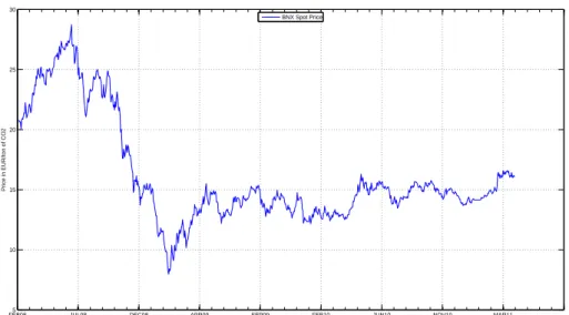
Figure 1 presents the daily time series of EUA Spot prices traded in =C/ton of CO2 on BlueNext (BNX) from February 26, 2008 to April 26, 2011 which

corresponds to a sample of 819 observations. The start of the study period corresponds to the trading of CO2 spot allowances valid during Phase II

under the EU ETS1_{.The EUA Spot prices are also presented in logreturn}

transformation in the bottom panel of Figure 1.

Descriptive statistics for all raw time-series and logreturns may be found

1

Phase I spot prices are not considered here, due to their non-reliable behavior (see Alberola and Chevallier (2009) for more details on the effects of inter-period banking restrictions on the price pattern of EUA spot prices during 2005-2007).

(4)

in Table 1. According to the Jarque-Bera test statistic, the distributional properties of the EUA Spot raw price series appear non-normal. In logre-turn transformation, the carbon futures are negatively skewed and since the kurtosis (or degree of excess) in exceeds three, a leptokurtic distribution is indicated. This comment applies in the remainder of the paper.

2.2 EUA Futures Price

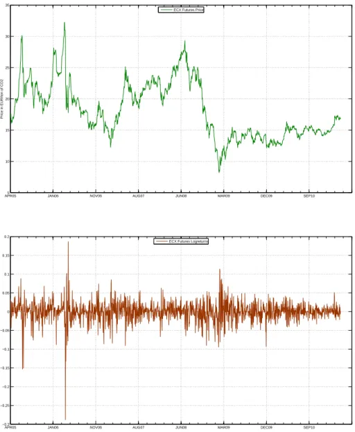
Figure 3 presents the daily time series of EUA Futures prices traded in =C/ton of CO2 on the European Climate Exchange (ECX) from April 22, 2005 to

April 26, 2011 which corresponds to a sample of 1,548 observations. The start of the study periods corresponds to the trading of CO2 futures allowances on

ECX. The EUA Futures prices are also presented in logreturn transformation in the bottom panel of Figure 3.

2.3 CER Futures Price

Figure 5 presents the daily time series of CER Futures prices traded in =C/ton of CO2 on ECX from March 09, 2007 to April 26, 2011 which corresponds to

a sample of 1,066 observations. The start of the study periods corresponds to the trading of CER futures allowances on ECX. The CER Futures prices are also presented in logreturn transformation in the bottom panel of Figure 5.

In what follows, we consider the log-return transformation of each time-series in the econometric analysis. In the next section, we present our esti-mation results.

(5)

3 Econometric Analysis

We explain first the basis of the econometric modelling with wavelet packet methods. Then, we detail the results obtained when applying this method-ology to carbon prices.

3.1 Wavelet Packet Transforms

In this section we base our exposition on, and borrow notation from, Na-son (2008) which draws on work on wavelet packet transforms by Wick-erhauser (1994), Coifman and WickWick-erhauser (1992), and Hess-Nielsen and Wickerhauser (1996). Besides, Percival and Walden (2000) have explained the discrete wavelet packet transform. Other useful contributions for time series analyses include Bernardini and Kovacevic (1996), Ombao et al. (2001, 2002, 2005). More recently, Gabbanini et al. (2004) have extended the def-inition of wavelet variance to wavelet packets, and introduced a method to discover variance change points based on wavelet packet variance2_.

Following the description in Coifman and Wickerhauser (1992), we start from a Daubechies mother and father wavelet, ψ and φ, respectively. Let W0(x) = φ(x) and W1(x) = ψ(x). Then, define the sequence of functions

{Wk(x)} ∞ k=0: W2n(x) = √ 2X k hkWn(2x − k) (1) 2

On a related topic, we may also cite the pioneering work on multiple wavelets by Geronimo et al. (1994), Strang and Strela (1994,1995), Xia et al. (1996) and Strela et al. (1999).

(6)

W2n+1(x) =

√ 2X

k

gkWn(2x − k) (2)

These equations correspond to the description that both hk and gk are

applied to W0 = φ and both to W1 = ψ, and then both hkand gk are applied

to the results of these.

Coifman and Wickerhauser (1992) define the library of wavelet packet bases to be the collection of orthonormal bases3 _{comprised of (dilated and}

translated versions of Wn) functions of the form Wn(2jx− k), where j, k ∈ Z

and n ∈ N. Here, j and k are the scale and translation numbers respectively, and n is a new kind of parameter called the number of oscillations. Hence, they conclude that Wn(2j − k) should be (approximately) centered at 2jk,

have support size proportional to 2−j

, and oscillate approximately n times. The definition of wavelet packets in eq. (1) and (2) shows how coeffi-cients/basis functions are obtained by the repeated application of filters to the original data (see Nason (2008) for a visual explanation of this mecha-nism).

3.2 Empirical Results

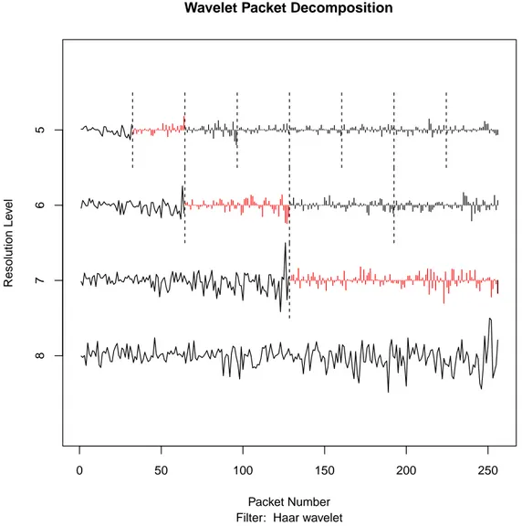
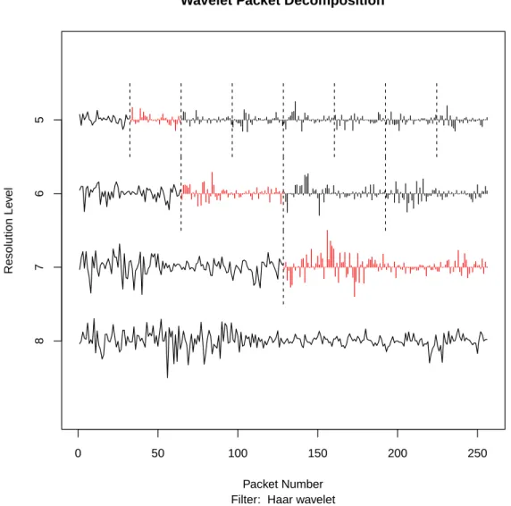
This modelling approach produces the wavelet packet plots shown in Figures 2, 4 and 6 for EUA Spot, EUA Futures and CER Futures prices, respectively. Turning to the scale 7 wavelet details in Figure 2 (for EUA Spot prices), we note that they are able to capture the period of strong adjustment to the recession, approximately from January 2009 onwards. At the smallest

3

See also Coifman and Wickerhauser (1992) for a formal definition of an orthonormal basis.

(7)

scale 5, we observe a clear rupture in February-April 2008, corresponding to the compliance event for the year 2007 on the European carbon market (see Chevallier (2011a) for a review of the calendar of compliance events on this market). At the intermediate scale 6, we can see an additional signfi-cant rupture in October-November 2008, corresponding to rising uncertain-ties concerning post-Kyoto agreements which were going to be discussed at the COP/MOP Summit in Poznan (Poland) in December of the same year.

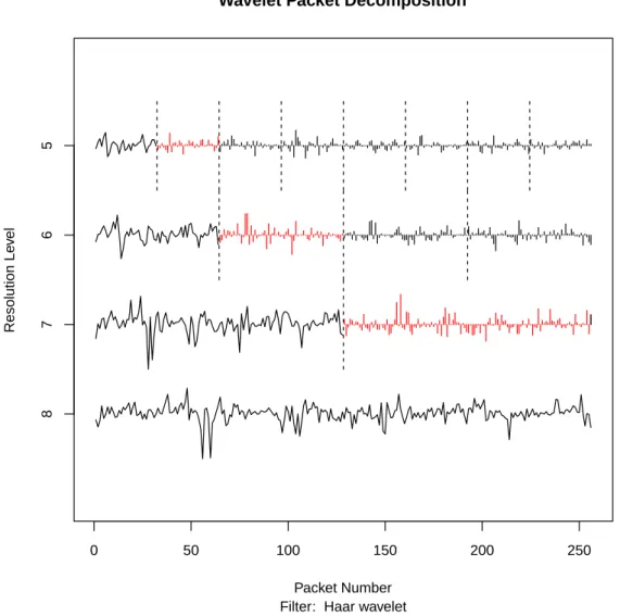
Let us now look at the wavelet details in Figure 4 (for EUA Futures prices). The estimation results are roughly similar, although at scale 7 smaller shocks are detected into CO2 futures price movements throughout

the recent 2009-2011 period covering the adjustment to the economic reces-sion and the slight economic uptake. The difference between spot and futures prices for the same asset may indeed be summarized as follows: while spot prices embody expectations about current events and shocks (on the phys-ical market for the commodity), futures prices reflect a longer-term view and larger set of information about market agents’ expectations of future events (such as the shape of international climate negotiation mechanisms until 2020).

Another feature which can be observed from Figure 6 (for CER Futures prices) is the larger variations at scales 6 and 7, which occur during 2008-2009 and exhibit more peaks than for EUA spot and futures price series. This result does not constitute a surprise in itself, as CERs are characterized by an even greater level of uncertainty than EUAs since there is no post-Kyoto scheme confirmed after 2012 (but the validity of CERs use for compliance in the EU ETS has been confirmed during 2013-2020, see Chevallier (2011b)).

(8)

4 Conclusion

While most previous studies rely on standard time-series analysis to study the empirical properties of carbon prices, this paper uses a more innovative approach based on wavelet packet transforms. Such a decomposition analysis has been found to be useful in previous literature to decompose a signal into various time scales, without losing time-related information, and to capture the various time scales at which the factors that influence the carbon price operate.

We show that the periods that have contributed the most to carbon price variations over Phase I and currently Phase II are:

• February-April 2008: for EUA spot prices, this corresponds to the 2007 compliance event;

• October-November 2008: for EUA spot prices, this corresponds to rising uncertainties about post-Kyoto negotiations before the Poznan summit;

• the recent 2009-2011 period: for EUA futures prices, this corresponds to a period of adjustment to the economic recession and timid recovery; • 2008-2009: for CER futures prices, this corresponds to similar kinds of

uncertainties concerning the status of the CDM post-2012.

These oscillations seem to occur mostly during periods of strong insti-tutional uncertainties. They also correspond to the time scales of business cycles. We may therefore conclude that carbon price variations are mainly driven by institutional events and macroeconomic fundamentals.

(9)

References

Alberola, E., Chevallier, J. 2009. European Carbon Prices and Banking Re-strictions: Ev-idence from Phase I (2005-2007). The Energy Journal 30(3), 51-80.

Bernardini, R., Kovacevic, J. 1996. Local orthogonal bases II: window design. Multidimensional systems and signal processing 7, 371-399.

Chevallier, J. 2011a. The European Carbon Market (2005-2007): Bank-ing, Pricing and Risk-Hedging Strategies. in Handbook of Sustainable Energy, Chapter 19, edited by Galarraga, I., Gonzalez-Eguino, M., Markandya, A. Edward Elgar.

Chevallier, J. 2011b. The Clean Development Mechanism: A Stepping Stone Towards World Carbon Markets? in Handbook of Sustainable Energy, Chapter 20, edited by Galarraga, I., Gonzalez-Eguino, M., Markandya, A. Edward Elgar.

Coifman, R.R., Wickerhauser, M.V. 1992. Entropy-based algorithms for best-basis selection. IEEE Transactions on Information Theory 38, 713-718. Gabbanini, F., Vannucci, M., Bartoli, G., Moro, A. 2004. Wavelet packet methods for the analysis of variance of time series with applications to crack widths on the Brunelleschi dome. Journal of Computational and Graphical Statistics 13, 639-658.

Geronimo, J.S., Hardin, D.P., Massopust, P.R. 1994. Fractal functions and wavelet expansions based on several scaling functions. Journal of Ap-proximation Theory 78, 373-401.

Hess-Nielsen, N., Wickerhauser, M.V. 1996. Wavelets and timefrequency analysis. Proceedings of the IEEE 84, 523-540.

Hunt, K., Nason, G.P. 2001. Wind speed modelling and short-term pre-diction using wavelets. Wind Engineering 25, 55-61.

Lee, J. 2005. Estimating memory parameter in the US inflation rate. Economics Letters 87(2), 207-210.

(10)

Nason, G.P., Sapatinas, T., Sawczenko, A. 2001. Wavelet packet mod-elling of infant sleep state using heart rate data. Sankhya B 63, 199-217.

Ombao, H., von Sachs, R., Guo, W.S. 2005. SLEX analysis of multivariate nonstationary time series. Journal of the American Statistical Association 100, 519-531.

Ombao, H.C., Raz, J., von Sachs, R., Malow, B.A. 2001. Automatic statistical analysis of bivariate nonstationary time series. Journal of the American Statistical Association 96, 543-560.

Ombao, H.C., Raz, J., von Sachs, R., Guo, W. 2002. The SLEX model of non-stationary random processes. Annals of the Institute of Statistical Mathematics 54, 171-20.

Percival, D.B., Walden, A.T. 2000. Wavelet Methods for Time Series Analysis. Cambridge University Press.

Strang, G., Strela, V. 1994. Orthogonal multiwavelets with vanishing moments. Optical Engineering 33, 2104-2107.

Strang, G., Strela, V. 1995. Short wavelets and matrix dilation equations. IEEE Transactions on Signal Processing 43, 108-115.

Strela, V., Heller, P.N., Strang, G., Topiwala, P., Heil, C. 1999. The ap-plication of multiwavelet filterbanks to image processing. IEEE Transactions on Image Processing 8, 548-563.

Wickerhauser, M.V. 1994. Adapted Wavelet Analysis from Theory to Software. A.K. Peters.

Wu, H. 2006. "Wavelet Estimation of Time Series Regression with Long Memory Processes. Economics Bulletin 3(33), 1-10.

Xia, X.G., Geronimo, J., Hardin, D., Suter, B. 1996. Design of prefilters for discrete multiwavelet transforms. IEEE Transactions on Signal Process-ing 44, 25-35.

Yogo, M. 2008. Measuring business cycles: A wavelet analysis of economic time series. Economics Letters 100(2), 208-212.

(11)

B N X S P O T B N X S P O T R E T E C X E U A F U T E C X E U A F U T R E T E C X C E R F U T E C X C E R F U T R E T M ea n 1 6 .1 5 7 6 -0 .0 0 0 3 1 8 .2 2 6 4 -0 .0 0 0 1 1 4 .0 9 3 4 0 .0 0 0 1 M ed ia n 1 4 .6 8 0 0 0 .0 0 0 1 1 7 .4 5 0 0 0 .0 0 0 1 1 3 .3 3 5 0 0 .0 0 0 1 M a x im u m 2 8 .7 3 0 0 0 .1 0 5 4 3 2 .2 5 0 0 0 .1 8 6 5 2 2 .8 5 0 0 0 .1 1 2 5 M in im u m 7 .9 6 0 0 -0 .1 0 2 8 8 .2 0 0 0 -0 .2 8 8 2 7 .4 8 4 6 -0 .1 1 0 4 S td . D ev . 4 .3 7 0 6 0 .0 2 3 3 4 .4 5 9 4 0 .0 2 6 5 2 .8 0 5 5 0 .0 2 1 1 S k ew n es s 1 .1 9 7 0 -0 .2 0 6 5 0 .4 5 2 9 -0 .9 8 0 2 0 .7 6 6 0 -0 .3 4 0 9 K u rt o si s 3 .3 4 6 3 5 .4 2 9 4 2 .4 0 0 8 1 6 .0 1 7 4 3 .0 6 9 1 6 .3 0 4 8 J a rq u e-B er a 1 9 9 .6 8 8 7 2 0 6 .9 7 5 3 7 6 .0 9 4 2 1 1 1 7 0 .4 9 0 0 1 0 4 .4 6 80 5 0 5 .3 0 8 9 P ro b . 0 .0 0 0 0 0 .0 0 0 0 0 .0 0 0 0 0 .0 0 0 0 0 .0 0 0 0 0 .0 0 0 0 O b s. 8 1 9 8 1 8 1 5 4 8 1 5 4 7 1 0 6 6 1 0 6 5 T ab le 1: D es cr ip ti ve st at is ti cs N o te : B N X S P O T re fe rs to th e B N X S p o t ti m e se ri e s in ra w fo rm , B N X S P O T R E T to th e B N X S p o t ti m e se ri e s in lo g re tu rn tr a n sf o rm a ti o n , E C X E U A F U T re fe rs to th e E U A F u tu re s ti m e se ri e s in ra w fo rm , E C X E U A F U T R E T to th e E U A F u tu re s ti m e se ri e s in lo g re tu rn tr a n sf o rm a ti o n , E C X C E R F U T to th e E C X C E R F u tu re s ti m e se ri e s in ra w fo rm , E C X C E R F U T R E T to th e E C X C E R F u tu re s ti m e se ri e s in lo g re tu rn tr a n sf o rm a ti o n , S td . D e v . to st a n d a rd d e v ia ti o n , P ro b . to th e p ro b a b il it y o f th e J a rq u e -B e ra te st , a n d O b s. to th e n u m b e r o f o b se rv a ti o n s.

(12)

FEB085 JUL08 DEC08 APR09 SEP09 FEB10 JUN10 NOV10 MAR11 10 15 20 25 30

Price in EUR/ton of CO2

BNX Spot Price

FEB08 JUL08 DEC08 APR09 SEP09 FEB10 JUN10 NOV10 MAR11

−0.2 −0.15 −0.1 −0.05 0 0.05 0.1 0.15 BNX Spot Logreturns

Figure 1: Time series of BNX Spot daily closing prices in raw form (top) and logreturn transformation (bottom) from February 26, 2008 to April 26, 2011 Source: BlueNext

(13)

0 50 100 150 200 250

Wavelet Packet Decomposition

Filter: Haar wavelet Packet Number Resolution Le v el 8 7 6 5

Figure 2: Wavelet decomposition for BNX Spot daily closing prices in logre-turn transformation from February 26, 2008 to April 26, 2011

Note: The time series at the bottom of the plot, scale eight, depicts the original data. At scales seven through five different wavelet packets are separated by vertical dotted lines. The first packet at each scale corresponds to scaling function coefficients, and these have been plotted as a time series rather than a set of small vertical lines. The regular wavelet coefficients are always the second packet at each scale.

(14)

APR055 JAN06 NOV06 AUG07 JUN08 MAR09 DEC09 SEP10 10 15 20 25 30 35

Price in EUR/ton of CO2

ECX Futures Price

APR05 JAN06 NOV06 AUG07 JUN08 MAR09 DEC09 SEP10

−0.3 −0.25 −0.2 −0.15 −0.1 −0.05 0 0.05 0.1 0.15 0.2

ECX Futures Logreturns

Figure 3: Time series of ECX EUA Futures daily closing prices in raw form (top) and logreturn transformation (bottom) from April 22, 2005 to April 26, 2011

(15)

0 50 100 150 200 250

Figure 4: Wavelet decomposition for ECX EUA Futures daily closing prices in logreturn transformation from April 22, 2005 to April 26, 2011

(16)

MAR076 DEC07 DEC08 JUL09 APR10 JAN11 8 10 12 14 16 18 20 22 24

ECX CER Futures

MAR07 DEC07 DEC08 JUL09 APR10 JAN11

−0.2 −0.15 −0.1 −0.05 0 0.05 0.1 0.15

ECX CER Logreturns

Figure 5: Time series of ECX CER Futures daily closing prices in raw form (top) and logreturn transformation (bottom) from March 09, 2007 to April 26, 2011

(17)

0 50 100 150 200 250

Figure 6: Wavelet decomposition for ECX CER Futures daily closing prices in logreturn transformation from March 09, 2007 to April 26, 2011