AP and MN-centric Mobility Prediction:
A Comparative Study Based on Wireless Traces
Jean-Marc Fran¸cois and Guy Leduc Research Unit in Networking (RUN)
Department of Electrical Engineering and Computer Science Institut Montefiore, B28 — Sart-Tilman
University of Li`ege 4000 Li`ege, Belgium
{francois,leduc}@run.montefiore.ulg.ac.be
Abstract. The mobility prediction problem is defined as guessing a mo-bile node’s next access point as it moves through a wireless network. Those predictions help take proactive measures in order to guarantee a given quality of service. Prediction agents can be divided into two main categories: agents related to a specific terminal (responsible for antici-pating its own movements) and those related to an access point (which predict the next access point of all the mobiles connected through it). This paper aims at comparing those two schemes using real traces of a large WiFi network. Several observations are made, such as the difficul-ties encountered to get a reliable trace of mobiles motion, the unexpect-edly small difference between both methods in terms of accuracy, and the inadequacy of commonly admitted hypotheses (such as the different motion behaviours between the week-end and the rest of the week).
1
Introduction
Wireless networks have experienced spectacular developments those last ten years. They are today facing two major changes:
– The number of wireless users grows quickly, and those users always ask for more bandwidth. The current trend is thus to reduce the transmitters’ coverage which in turn increases the rate at which mobile hosts (MHs) switch from an antenna to the next (or handover rate).
– Since voice, television, and data networks are now merging, it would be desirable to be able to guarantee various quality of service (QoS) levels. When a mobile terminal moves, one of the main causes of service degradation is switching between the network’s access points (APs): changing one’s current AP requires re-routing the received and sent data flows, a procedure which is This work has been supported by the Belgian Science Policy in the framework of the IAP program (Motion P5/11 project) and by the IST-FET ANA project.
likely to cause packet losses and delays. Predicting a MH’s next handover(s) allows taking pro-active measures to reduce handovers impact, a problem known as mobility prediction. In the following, we study a wireless WiFi network and aim at predicting each mobile host’s next AP.
Mobility prediction methods can be classified into two main families: – MH-centric (MHC): the agent performing predictions is bound to a MH;
it builds a model of this particular MH’s movements (e.g. [1,2,3]);
– AP-centric(APC): the prediction agent is bound to an AP; this AP builds a model using the motion of the MHs passing by (e.g. [4,5,6]).
Those models can be built on-line, as the mobiles move, and can perform a prediction anytime.
The pieces of information that allow deducing the likely motion of a mobile terminal are very varied (e.g. GPS coordinates). In what follows, we assume that the piece of information used is the sequence of most recently encountered APs. This assumption is not strong since it only requires that MHs record the last APs they have been associated with.
The various prediction methods presented in the literature have rarely been validated using mobility traces extracted from a real network. [7] is a notable exception which shows that simple markovian models perform nearly as well as other, more complex methods. We thus focus on those models in this paper.
In the following, we present a comparison between MH and AP-centric pre-diction methods using the mobility traces of a large-scale WiFi network. It is expected that the conclusions drawn here could be applied to other kinds of mobile networks.
The rest of the paper is organised as follows. Section 2 defines the prediction models utilized in the article. Sections 3 and 4 give a description of the traces used, the way they have been processed, and basic performance results. Sec-tion 5 compares both types of predicSec-tion schemes (MHC and APC). SecSec-tion 6 concludes.
2
Next-AP predictors
A next-AP predictor, or prediction agent, is the entity responsible for building a model of MH’s movements; this model can be used for predictive purposes.
2.1 Centralized and decentralized methods
In this paper, we study the differences between the two most popular prediction schemes.
In the first method, APC, the prediction agents are the APs. Each AP builds a model of the movements of mobiles passing by. The MHs’ involvement is mini-mal, since they only send during each handover an identification of their previous APs. This architecture is particularly well suited to situations where predictions
are mainly useful to the fixed network infrastructure (which could, for example, use it to reserve resources anticipatively).
The second method, MHC, is more distributed: every MH builds a model using its own movements. It is expected to be more reliable since more specific: the behaviour of a particular mobile cannot be simplified to the mean behaviour of all the MHs moving in the same area. However, this scheme does not fit well the standard wireless network paradigm, where terminals are supposed to be small, memory and processing limited devices (such as a low-end GSM), and not suited to running a learning algorithm. Moreover, no prediction can be made when a MH visits APs for the first time.
2.2 Markovian models
We model MHs’ motion habits thanks to their location history (or trace), i.e. the sequence of APs crossed during their journey. Considering each AP as a symbol of a (finite) alphabet, a MH’s trace is a sequence of symbols and prediction aims at guessing symbol i + 1 given the first i.
Observing MHs’ motion allows a prediction agent to tune the model’s pa-rameters so that prediction improves over time
It has been shown ([7,8]) that in this context, simple Markov predictors perform as well as other, more complex methods1
(such as [9,10,11,12]). We thus only consider this class of predictors here.
Let L = {L1, L2, L3. . .} be the set of locations and L = L1, L2, L3. . . a
location history. The order n markovian hypothesis is:
P(Li= l|L1, . . . , Li−1) = P (Li = l|Li−n, . . . , Li−1) ∀ l ∈ L, i > n (1)
Less formally, this equation states that the stochastic variable that describes the next-AP probability follows a distribution that only depends on the last n symbols. We assume a stationary distribution2
.
The next-AP distribution can easily be learnt on-line. We assume that the agent responsible for building the markovian model is regularly notified of MH(s) movements.
If we denote Lm
the location history of mobile m, the order-n model estima-tion rule is:
P(Li= l | Li−n, . . . , Li−1) = P m∈MO(L m i−n, . . . , L m i−1, l; L m ) P m∈MO(L m i−n, . . . , L m i−1; L m) (2)
where the O(· ; ·) operator finds the number of occurrences of its first argument in its second, and M is the set of mobiles involved.
In the case of MHC, each terminal only models its own motion, thus M is a singleton.
1
To be fair, some of those not only aim at location prediction, but at other purposes such as mobile paging.
2
When a model is used to perform a prediction, the most probable next AP (given the current context, i.e. the MH’s last n APs) is chosen. No prediction can be performed if the context has never been observed before. To limit the consequences of this possibility, we build together with each order-n model, n−1 other models of order n − 1, n − 2, . . . , 1. If a prediction cannot be performed because the current context is seen for the first time, we fallback on a lower-order model.
We do not aim at predicting when a mobile will enter or leave the network; only the proper inter-AP movements are taken into account.
...
...
...
<AP3, AP4> <AP3 AP4, AP5> <AP4 AP5, AP9> <AP4, AP5>... Learning set Learning set AP4 order 2 models order 1, AP1 order 2 models order 1, APC agents Learning set Learning set MH2 order 2 models order 0, order 1, MH1 order 2 models order 0, order 1, MHC agents AP3 AP7 AP8 AP4 AP5 AP6 MH1 trace: MH2 trace:
AP3 AP4 AP7 AP8...
AP3 AP4 AP5 AP9 OFF AP4 AP5... <AP3, AP4> <AP3 AP4, AP7> <AP4 AP7, AP8>...
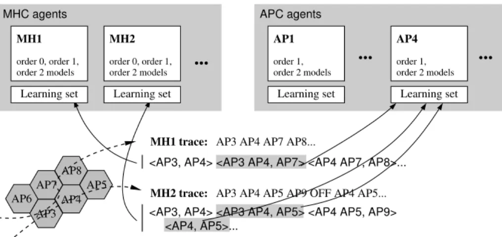
Fig. 1. Overview of the learning process for order-2 markovian models. The mobiles’ motion generates location histories that allow agents to build a set of “context, next-AP” couples (here denoted between brackets). The special “OFF” AP is introduced when the MH leaves the network; since we do not aim at predicting this event, those APs do not appear in the learning sets.
3
Wireless traces
The traces used have been collected by Dartmouth University in the context of the CRAWDAD project ([13]). It is a collection of events generated by the WiFi network of the campus. Syslog and SNMP data have been recorded for 2 years and cover 6202 MHs and 575 APs ([14]).
This data have been analysed ([8]) to extract the actual movement traces (i.e. for each MH, a sequence of APs). A special AP, denoted OFF, indicates that a mobile has been ’deauthenticated’ or that it has not generated any activity since at least 30 minutes; we then consider that it has been disconnected.
Each MH is identified using its MAC address; we assume that each MAC address matches one (and only one) user. Apparatus with more than one interface and apparatus shared by more than one person are considered rare.
In the following, the same data are exploited to perform MH and AP-based predictions. More formally, each time MH m moves, its last n movements Lm
i−n, . . . , L m
i−1 and the next AP L m
i are used to learn the parameters of an
order-n markovian model; those “context, next AP” couples are the elements (or learning samples) of the learning set. With MHC, the prediction agent is bound to ’m’; with APC, it is bound to Lm
i−1. Notice that the contexts fed to
Lm
i−1always end with L m
i−1; an order n model built with APC is thus as complex
as an order n − 1 model built using MHC.
Figure 1 depicts graphically the learning process. Each time a terminal moves, its new AP is appended to its mobility trace; a special ’OFF’ AP is added when the MH is disconnected from the network. This trace is then converted to a series of “context, next-AP” couples; the maximal context length depends on the order of the models built. The couples corresponding to MH m populate the learning set bound to m (left); the couples whose context ends with AP p are the learning samples that compose the learning set of p’s agent (right).
0 2 4 6 8 10 12 14 16 256K 64K 16K 4K 1K 256 64 16 4 1 Frequency (%)
Learning set cardinality
MH-centric modelling 0 2 4 6 8 10 12 14 256K 64K 16K 4K 1K 256 64 16 4 1 Frequency (%)
Learning set cardinality
AP-centric modelling
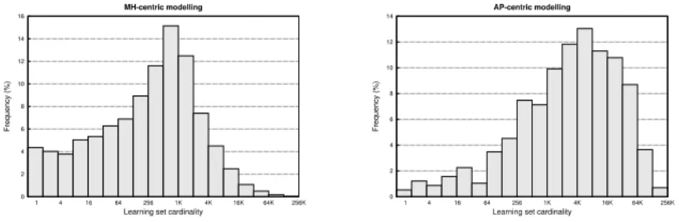
Fig. 2. Distributions of learning sets cardinalities regarding MHC (left) and APC (right). The x-axis is logarithmic.
Figure 2 compares APC and MHC in terms of the distributions of the learning sets’ cardinality (i.e. the number of “context, next AP” couples). A lot of MHs barely move: 12% perform less than 8 movements (plot on the left, sum of the percentages reported in the first 3 bars). On the contrary, few APs are unpopular: 15% are crossed by less than 256 MHs. The impact of under-learning should thus be more pronounced using the distributed MHC method.
3.1 Ping-ponging
It is known (e.g. [15]) that such dataset exhibits the ping-ponging artefact (ping-ponging is defined as repeatedly changing one’s current association back and forth between two —or more— access points).
Mobility prediction is concerned about the physical movements of mobile terminals, not about those quick artefacts. This does not mean that predicting
ping-ponging is not an interesting topic, but that it is only marginally related to the question studied here. We thus try to remove this artefact.
Considering the location history L1, . . . , Ln of a MH, the movement to Ln
is classified as ping-ponging if Ln−2 = Ln. This simple rule surely does trigger
“false positive”: MHs physically moving back and forth from an AP to another are classified as ping-ponging. However, we notice that the proportion of move-ments classified as ping-ponging varies from one interface manufacturer to an-other. Our criterion thus looks reasonable since it filters handovers triggered by a technological cause. About 3 movements out of 10 are classified as ping-ponging.
4
Next-AP predictions accuracy
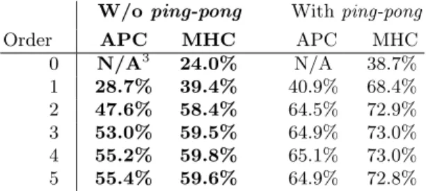
Table 1 shows the next-AP prediction accuracy using both APC and MHC, for various model orders.
W/o ping-pong With ping-pong
Order APC MHC APC MHC
0 N/A3 24.0% N/A 38.7% 1 28.7% 39.4% 40.9% 68.4% 2 47.6% 58.4% 64.5% 72.9% 3 53.0% 59.5% 64.9% 73.0% 4 55.2% 59.8% 65.1% 73.0% 5 55.4% 59.6% 64.9% 72.8%
Table 1. Prediction accuracy. Each number corresponds to the ratio between the number of accurate predictions and the total number of predictions. The columns on the right show the performance one would obtain if ping-ponging were not removed.
We first observe that a simple, statistical approach4
gives unsatisfactory re-sults. Models improve quickly: order-2 models are quasi-optimal. Beyond that, performance improves very slowly and reaches its apogee with order-4 mod-els. Performance decreases with models of higher order, showing a slight over-learning. The columns on the right are those obtained if the ping-ponging move-ments are not removed; they show that ping-ponging is easy to predict, even with simple markovian models.
Results related to MHC are in accordance with [7]. Since table 1 shows that ping-ponging has a major impact on the prediction results, it would be inter-esting to repeat the experiments presented in [7] once ping-ponging has been filtered out.
3
An order n model is based on contexts of length n. With APC, the prediction agent is the same as the last element of the context, which is undefined in the case of a context of length 0.
4
The good prediction ratio is, overall, quite low. We can suppose that it would be higher for other kinds of networks where terminals are usually not switched off during their displacements (e.g. GSM), even if some of the terminals composing this dataset are WiFi phones ([14]). In this study, absolute accuracy performance is not our primary concern; we here emphasize the differences between APC and MHC schemes.
The decentralized MHC scheme works better than APC. This result was expected, as different persons have their specific behaviour: averaging the move-ment patterns of the people crossing the same AP only gives a rough estimate of the way they move. Surprisingly however, the accuracy difference between APC and MHC is small (from 55.4% to 59.8%); in practice, this means that getting decent prediction performance does not require to embed a prediction agent in each mobile: placing them in the fixed infrastructure can suffice. Section 5.2 gives hints on why the results of the two methods are so close.
5
Stressing the differences between APC and MHC
5.1 Prediction accuracy vs learning set cardinality
The markovian models’ parameters learning process and the prediction process are interleaved: when a mobile is associated with an AP, this AP predicts where the terminal is going; as soon as the next AP is known, this piece of information is added to the learning set and allows it to improve the mobility model. The ratio of accurate predictions is thus a function of the elapsed learning time, and the way it evolves depends on the method used — APC or MHC.
90 80 70 60 50 40 30 20 10 0 100 0.8 0.7 0.6 0.5 0.4 0.3 0.2 0.1 0 0 1000 2000 3000 4000 5000 6000 7000 8000 9000 MH (%)AP (%) MHCAPC Prediction accuracy
Learning set cardinality
Percentage of AP or MN
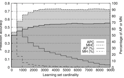
Fig. 3. Prediction accuracy (strong lines, left axis) and proportion of prediction agents (thin lines, right axis) vs learning sets’ cardinality using order 3 models.
Figure 3 (bold lines, left axis) draws the instantaneous prediction accuracy as a function of the learning sets cardinality. This plot shows that learning sets made of a few hundred elements lead to prediction ratios of more than 40%, regardless of whether prediction agents depend on APs or MHs. For bigger learning sets, both methods show different profiles. For APC, performance gets slowly better and stabilizes at 55% when the learning set is made of about 3000 samples. With MHC, the results increase much faster, reaching 60% when the learning set is composed of 1000 elements, and settling at about 73% with 2000 elements. This last percentage is astonishingly good and is thus studied more carefully below.
On the same figure, thin lines (right axis) give the proportion of prediction agents which have a learning set cardinality higher than a given value. For ex-ample, for MHC, about 80% of the mobiles have a learning set composed of less than 500 elements. The curve associated with MHC decreases much faster than that of APC: nearly all the models have a learning set with a cardinality smaller than 3000. The APC curve has a very different shape: there are still some learning sets with cardinalities greater than 8000 elements. Only a small number of MHs are thus responsible for prediction ratios higher than 70%. A manual inspection of motion traces shows that ping-ponging between 3 APs or more seems to explain this anomaly. Fortunately, this situation is rare and should only marginally impact the average performance.
This figure allows finding the steady-state (i.e. on the long run) good pre-diction ratio reached by each method. If APC clearly settles at about 55%, the case of MHC needs to be considered more carefully. As mentioned above, per-formance of 70% or more are not realistic. We thus remove the 10% of best performing MHs and measure the performance of the remaining mobiles once they have reached a learning set cardinality greater than 500 elements; the good prediction ratio obtained is then 60.8%.
5.2 Next-AP distributions’ entropy
Knowing the last APs encountered by a mobile terminal (or context) does not allow a perfect prediction of its next AP. This uncertainty can be formalized as a random distribution of next APs; this distribution is characterized by a given entropy. This entropy is commonly linked to the difficulty of predicting the motion of the mobile.
Mean entropies of order 1, 2, and 3 models are given in table 2 for APC and MHC.
Method 1 2 3
APC 1.86 (0.95) 1.72 (1.18) 1.58 (0.49) MHC 0.98 (0.50) 0.82 (0.66) 0.91 (0.37)
Table 2. Next-cell distribution entropies (in bits). Standard deviations are given be-tween parentheses.
The two schemes exhibit strong differences. This runs counter to the results obtained in terms of prediction accuracy (see table 1) which showed a difference indeed, but as small as about 5%. From this experiment, we can conclude that MHC clearly predicts more precisely which APs might be next encountered by a MH, but this problem is different from the one generally studied, which is only concerned with finding the most probable next AP. Thus, even if entropy estimation allows us to get a quantitative measurement of the mobiles’ motion uncertainty given a model, directly linking entropy to prediction accuracy gives a biased picture. A more complete study of this point can be found in [16].
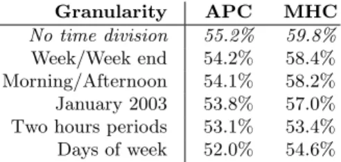
5.3 Time division
It is commonly supposed (e.g. [17]) that it is desirable to divide a learning set in homogeneous time slices: it seems for example sensible to expect different motion behaviours during the week-end and during the rest of the week, and it is thus reasonable to build different models for those periods of time.
Granularity APC MHC
No time division 55.2% 59.8%
Week/Week end 54.2% 58.4%
Morning/Afternoon 54.1% 58.2%
January 2003 53.8% 57.0%
Two hours periods 53.1% 53.4%
Days of week 52.0% 54.6%
Table 3. Prediction accuracy when different order 4 models are built for various time divisions. The results given are the (weighted) mean performance of the models built.
Using such a method would however bring two drawbacks: (a) the start of the model’s learning curve could cause bad performance, and (b) short time periods could yield too small learning sets.
Table 3 gives the results obtained using various time divisions.
The results are surprising: in no case do the time slices improve the results. Two hypotheses can explain this fact: (a) the MHs’ behaviours are the same during all the time periods (movements are not cyclic and can be described as a stationary process) or (b) the motion context already captures those differences.
6
Conclusions and future works
Mobility prediction schemes can be divided into two main classes, here des-ignated AP-centric (or centralized) and MH-centric (or decentralized). Quite surprisingly, they have never been directly quantitatively compared.
This article partially fills this gap using a study based on markovian models. The parameters of those models are fit via the analysis of a database containing the real motion traces of the mobile hosts of a campus WiFi network.
It allows us to draw a number of conclusions:
– Contrary to one could expect, the measured accuracy difference between APC and MHC is only a few percents (typically 55% vs 59%).
– In any case, the prediction accuracy is low (less than 60%); this is certainly a characteristic of WiFi users, and we expect other networks (e.g. GSM) to exhibit more predictable, regular motion patterns. This is not a real concern for this study as we are more interested in comparing APC and MHC rather than in absolute results.
– Next-AP prediction uncertainty can be estimated by an entropy measure-ment, but this only partially reflects prediction accuracy and, in this case, does not provide an accurate comparison of APC and MHC. One should thus refrain from linking entropy to prediction accuracy as this can introduce a bias.
– Quite surprisingly, we notice that building models specific to certain peri-ods of time (e.g. week/week-end, morning/afternoon) does not bring any improvement.
This comparison could be continued along several lines. For example, the relevance of an hybrid method combining APC and MHC schemes could be explored; the prediction of APC could, for example, be used when a MH reaches an AP it has never seen before. This situation barely arises in the dataset used here, hence such an experiment should be tried using traces extracted from a different network.
References
1. Misra, A., Roy, A., Das, S.: An information-theoretic framework for optimal loca-tion tracking in multi-system 4G networks. In: Proc. of INFOCOM’04. (2004) 2. Laasonen, K.: Clustering and prediction of mobile user routes from cellular data.
PKDD 2005, LNAI 3721 (2005) 569–576
3. Samaa, N., Karmouch, A.: A mobility prediction architecture based on contex-tual knowledge and spatial concepcontex-tual maps. IEEE Trans. on mobile comp. 4 (November/December 2005)
4. Hadjiefthymiades, S., Merakos, L.: Using path prediction to improve TCP perfor-mance in wireless/mobile communications. IEEE Communications 40(8) (August 2002)
5. Soh, W.S., Kim, H.: Dynamic bandwidth reservation in cellular networks using road topology based mobility predictions. In: Proc. of IEEE INFOCOM’04. (Mars 2004)
6. Pandey, V., Ghosal, D., Mokherjee, B.: Exploiting user profile to support differ-entiated services in next-generation wireless networks. IEEE Network (Septem-ber/October 2004)
7. Song, L., Kotz, D., Jain, R., He, X.: Evaluating location predictors with extensive Wi-Fi mobility data. Technical Report TR2004-491, Dartmouth College (February 2004)
8. Song, L., Kotz, D., Jain, R., He, X.: Evaluating location predictors with extensive Wi-Fi mobility data. In: Proc. of 23rd Annual Joint Conference of the IEEE Computer and Communications Societies. Volume 2. (March 2004) 1414–1424 9. Bhattacharya, A., Das, S.: LeZi-update: an information-theoretic approach to track
mobile users in PCS networks. In: Proc. of MobiCom’99, Seattle (August 1999) 10. Yu, F., Leung, V.: Mobility-based predictive call admission control and bandwidth
reservation in wireless cellular networks. Computer Networks 38(5) (2002) 11. Cleary, J.G., Witten, I.H.: Data compression using adaptive coding and partial
string matching. IEEE Transactions on Communications 32(4) (1984) 396–402 12. Jacquet, P., Szpankowski, W., Apostol, I. In: An universal predictor based on
pattern matching, preliminary results. (2000) 75–85
13. Kotz, D.: CRAWDAD, a Community Resource for Archiving Wireless Data At Dartmouth. http://crawdad.cs.dartmouth.edu/ (2005)
14. Kotz, D., Essien, K.: Analysis of a campus-wide wireless network. In: MobiCom. (September 2002) 107–118 Revised and corrected as Technical Report TR2002-432. 15. Conan, V., Leguay, J., Friedman, T.: The heterogeneity of inter-contact time
distributions [. . . ]. arXiv.org, cs/0609068 (2006)
16. Fran¸cois, J.M.: Performing and Making use of Mobility Prediction. PhD thesis, University of Li`ege (2007)
17. Choi, S., Shin, K.: Predictive and adaptive bandwidth reservation for hand-offs in QoS-sensitive cellular networks. SIGCOMM CCR 28(4) (1998) 155–166