TDCOSMO. II. Six new time delays in lensed quasars from high-cadence monitoring at the MPIA 2.2 m telescope

https://doi.org/10.1051/0004-6361/202038698 c ESO 2020

Astronomy

&

Astrophysics

TDCOSMO

II. Six new time delays in lensed quasars from high-cadence monitoring at the

MPIA 2.2 m telescope

?

M. Millon

1

, F. Courbin

1

, V. Bonvin

1

, E. Buckley-Geer

2,4

, C. D. Fassnacht

3

, J. Frieman

2,4

, P. J. Marshall

5

,

S. H. Suyu

6,7,8

, T. Treu

9

, T. Anguita

10,11

, V. Motta

12

, A. Agnello

13

, J. H. H. Chan

1

, D. C.-Y. Chao

6,7

, M. Chijani

10

,

D. Gilman

9

, K. Gilmore

5

, C. Lemon

1

, J. R. Lucey

14

, A. Melo

12

, E. Paic

1

, K. Rojas

1

, D. Sluse

17

, P. R. Williams

9

,

A. Hempel

10,16

, S. Kim

15,16

, R. Lachaume

15,16

, and M. Rabus

18,19

(Affiliations can be found after the references) Received 18 June 2020/ Accepted 21 August 2020

ABSTRACT

We present six new time-delay measurements obtained from Rc-band monitoring data acquired at the Max Planck Institute for Astrophysics (MPIA) 2.2 m telescope at La Silla observatory between October 2016 and February 2020. The lensed quasars HE 0047−1756, WG 0214−2105, DES 0407−5006, 2M 1134−2103, PSJ 1606−2333, and DES 2325−5229 were observed almost daily at high signal-to-noise ratio to obtain high-quality light curves where we can record fast and small-amplitude variations of the quasars. We measured time delays between all pairs of multiple images with only one or two seasons of monitoring with the exception of the time delays relative to image D of PSJ 1606−2333. The most precise estimate was obtained for the delay between image A and image B of DES 0407−5006, where τAB = −128.4+3.5−3.8d (2.8% precision) including systematics due to extrinsic variability in the light curves. For HE 0047−1756, we combined our high-cadence data with measurements from decade-long light curves from previous COSMOGRAIL campaigns, and reach a precision of 0.9 d on the final measurement. The present work demonstrates the feasibility of measuring time delays in lensed quasars in only one or two seasons, provided high signal-to-noise ratio data are obtained at a cadence close to daily.

Key words. gravitational lensing: strong – methods: data analysis – cosmological parameters

1. Introduction

Time-delay cosmography with strongly lensed quasars was first proposed byRefsdal(1964) as a single-step method to measure the Hubble constant H0. The method relies on three

ingredi-ents. First, a precise measurement of the time delays between the lensed images must be obtained. This is typically achieved from photometric monitoring campaigns producing the light curve for each multiple image. Second, a mass model is needed for the main lensing galaxy and its possible companions. Deep and high-resolution images, typically obtained with adaptive optics (AO) or the Hubble Space Telescope (HST) are needed for this task. Finally, we need to estimate the contribution of all intervening galaxies along the line of sight to the quasar. This last step can be performed statistically with galaxy counts in wide-field images (Rusu et al. 2017), direct multiplane modeling (McCully et al. 2017), or weak lensing measurements (e.g., Tihhonova et al. 2018). These three ingredients allow for direct measurements of distances to the lens system, which together with the lens and source redshift measurements, provide constraints on H0.

The method is complementary to other probes such as the cosmological microwave background (CMB), baryon acous-tic oscillation (BAO), and the cosmic distance ladder, since time-delay cosmography is mainly sensitive to H0 and depends

weakly on the other cosmological parameters. It is therefore an ideal probe to lift degeneracies in other experiments. Using lensed quasars, Wong et al. (2019) obtained a 2.4% precision

?

All light curves presented in this paper are only available at the CDS via anonymous ftp tocdsarc.u-strasbg.fr(130.79.128.5) or via http://cdsarc.u-strasbg.fr/viz-bin/cat/J/A+A/642/A193

on the Hubble constant in flat-ΛCDM cosmology with a sam-ple of six systems studied by the H0LiCOW collaboration (Suyu et al. 2010,2014; Wong et al. 2017; Bonvin et al. 2017; Birrer et al. 2019;Rusu et al. 2019;Chen et al. 2019). Combin-ing this measurement with the latest results from the Cepheid distance ladder (Riess et al. 2019), the tension with the Planck results (Planck Collaboration VI 2020) reaches 5.3σ, suggest-ing the presence of unaccounted systematics in one or both experiments or new physics beyond the ΛCDM model (e.g., Verde et al. 2019;Riess 2019;Freedman et al. 2020).

The COSMOGRAIL program has so far been one of the lead-ing projects dedicated to time-delay measurement in strong lens-ing systems. This program produced decade-long light curves of more than 20 objects with 1 m class telescopes, yielding many precise time-delay measurements (e.g.,Tewes et al. 2013a; Eulaers et al. 2013; Rathna Kumar et al. 2013; Bonvin et al. 2017). In particular, the final paper of the COSMOGRAIL series presents time delays for 18 objects (Millon et al. 2020). The observation strategy was recently enhanced with higher cadence (daily observation) and improved photometric precision and now allows us to catch quasar variations that are faster than the typical microlensing signal. Consequently, time delays can be measured to a few percent precision in only one monitoring season, pro-vided 2 m-class telescopes can be used on a daily basis. This is the case of the MPIA 2.2 m telescope at ESO La Silla Observatory, which we use in the present work. Previous results using this tele-scope and strategy were presented inCourbin et al.(2018) and Bonvin et al.(2018,2019).

In this paper, we report six new time delays with preci-sions in the range 2.8% hδ(∆t)/∆ti18.3%. We first present in

Table 1. Summary of the optical monitoring data in the Rcband.

Target zs zl Period of observation #Epochs Seeing Sampling Reference

HE 0047−1756 1.66 0.407 Oct. 2nd 2016–Jan. 23rd 2018 186 100

09 1.80 days Wisotzki et al.(2004) WG 0214−2105 3.24 ∼0.45 June 2nd 2018–Feb. 19th 2020 296 100_{08 1.50 days Agnello & Spiniello(2019)}

DES 0407−5006 1.515 – Aug. 3rd 2016–May 4th 2019 174 100

09 1.40 days Anguita et al.(2018)

2M 1134−2103 2.77 – Dec. 7th 2017–July 31st 2018 166 000

92 1.32 days Lucey et al.(2018)

PSJ 1606−2333 1.69 – Jan. 25th 2018–Sep. 23rd 2018 158 000

95 1.52 days Lemon et al.(2018)

DES 2325−5229 2.74 0.400 Apr. 14th 2018–Jan. 6th 2019 183 100

22 1.33 days Ostrovski et al.(2017)

TOTAL – – Oct. 2nd 2016–May. 4th 2019 1163 – – –

Notes. Each epoch consists of 4 exposures of 320 s each. The temporal sampling is the mean number of days between two consecutive observations (epochs), excluding the seasonal gap for HE 0047−1756 and WG 0214−2105. Column 6 corresponds to the median seeing measured in the images for each object. The seeing and airmass distributions are shown in Fig.1.

Sect. 2the high-cadence, high signal-to-noise ratio (S/N) light curves of the lensed quasars HE 0047−1756, WG 0214−2105, DES 0407−5006, 2M 1134−2103, PSJ 1606−2333, and DES 2325−5229, which were acquired between October 2016 and February 2020 at the MPIA 2.2 m telescope at La Silla. In Sect.4, we detail the time-delay measurement procedure before presenting and discussing our results in Sect. 5. Our conclu-sions are summarized in Sect. 7. This paper is the second of the TDCOSMO1 _{series, which includes the COSMOGRAIL}2_, H0LiCOW3_{, STRIDES}4 _{collaborations, and members of the} SHARP collaboration.

2. Observation and data reduction

The photometric monitoring data were acquired on a daily basis at the MPIA 2.2 m telescope at ESO La Silla. Each observing epoch consists of four dithered exposures of 320 s each, through the Rcfilter. The images were taken with the Wide Field Imager

(WFI) instrument, which is composed of eight charge-coupled devices (CCD) covering a field of view of 360× 360with a pixel size of 000_{238. A summary of the observing information is}

pre-sented in Table1and Fig.1.

The monitoring campaigns started in October 2016 and ran until February 2020 with a daily planned observing cadence. We observed a total of 11 targets for one full visibility season with the exception of HE 0047−1756, which was started in the middle of a season, and WG 0214−2105, for which two seasons were obtained. Among these 11 targets, 9 have sufficiently well-defined features in their light curves to measure the time delays. Three of these targets, namely DES 0408−5354, PG 1115+080, and WFI 2033−4723 are presented in previous COSMOGRAIL publications (Courbin et al. 2018;Bonvin et al. 2018,2019) and 6 are the topic of the present work. The remaining 2, namely SDSS J0832+0404 and DES 2038−4008, will require a second season of monitoring to obtain a robust time delay. These 2 objects are left for future work.

Our data were mainly taken when targets had an airmass below 1.5, but we sometimes relaxed the airmass requirement in order to extend the visibility window. A long seasonal coverage can be crucial in the case of long time delays, when the common features in the light curves only overlap by a few weeks. On aver-age over the six objects presented in this work, one data point per object was recorded every 1.48 d. The actual mean sampling of

1 _{www.tdcosmo.org}

2 _{www.cosmograil.org}

3 _{https://shsuyu.github.io/H0LiCOW/site/}

4 _{http://strides.astro.ucla.edu}

0.5 1.0 1.5 2.0 2.5

Seeing (per epoch) ["]

0.00 0.25 0.50 0.75 1.00 1.25 1.50 1.75

Normalised distribution

HE 0047-1756 WG 0214-2105 DES 0407-5006 2M 1134-2103 PSJ 1606-2333 DES 2325-5229 1.0 1.2 1.4 1.6 1.8

Airmass (per epoch)

0 1 2 3 4 5 6

Normalised distribution

HE 0047-1756 WG 0214-2105 DES 0407-5006 2M 1134-2103 PSJ 1606-2333 DES 2325-5229

Fig. 1.Seeing and airmass distributions for the six targets monitored with the WFI instrument at the MPIA 2.2 m telescope at ESO La Silla observatory.

the light curves is a bit larger than the scheduled daily cadence as a consequence of bad weather and technical maintenance of the telescope. The median seeing over the whole period reported is 100_06.

The data were reduced according to the standard COSMO-GRAIL5 _{procedure described in detail in Millon et al. (2020).}

5 _{The reduction pipeline can be found at the following address:www.} cosmograil.org

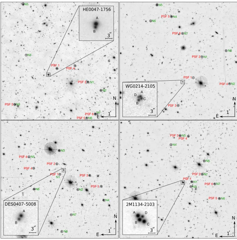
PSF 1 E N 1' HE0047-1756 A B 3'' PSF 2 PSF 3 PSF 4 PSF 5 PSF 6 N1 N2 N3 N4 N5 N6 N7 PSF 1 E N 1' WG0214-2105 A D B C 3'' PSF 2 PSF 3 PSF 4 PSF 5 PSF 6 N1 N2 N3 N4 N5 N6 N7 PSF 1 E N 1' DES0407-5008 A B 3'' PSF 2 PSF 3 PSF 4 PSF 5 PSF 6 N1 N2 N3 N4 N5 N6 N7 N8 PSF 1 E N 1' 2M1134-2103 A D B _C 3'' PSF 2 PSF 3 PSF 4 PSF 5 PSF 6 N1 N2 N3 N4 N5 N6 N7 N8

Fig. 2.Deep stacks of best-seeing images of HE 0047−1756 (74 images, with a total exposure time of 6.6 h), WG 0214−2105 (138 images, 12.3 h), DES 0407−5006 (82 images, 7.3 h), and 2M 1134−2103 (178 images, 15.8 h). The stars used to construct the PSF are circled and labeled in red, whereas the stars used for the night-to-night flux normalization are shown in green. The expanded boxes show single exposures of each lensed quasar in excellent seeing conditions, typically 000.6.

We first bias-subtracted and flat-fielded the images using sky flats. The sky level was then removed via the Sextractor soft-ware (Bertin & Arnouts 1996). As the WFI instrument is some-times affected by fringing in the Rc band, we also constructed

a fringe model by iteratively sigma-clipping the four dithered images taken at each epoch and by taking the median. This model was then subtracted from the four individual exposures.

To obtain an accurate photometric measurement in each sin-gle exposure, we performed image deconvolution of the quasar images with the MCS deconvolution algorithm (Magain et al.

1998;Cantale et al. 2016). This step largely improves the pho-tometric accuracy as the image separation between multiple images does not exceed a few arcseconds. Figures2and3show the stars used to compute the point spread function (PSF) as well as the reference stars used for image-to-image flux calibration. Each image was deconvolved individually with its own PSF, but all images share the same point source astrometry and the same “pixel” channel, which contains all extended sources such as the lensing galaxy, the quasar host galaxy, or companion galaxies (seeCantale et al. 2016, for detailed description of the method).

PSF 1 E N 1' PSJ 1606-2333 A D B C 3'' PSF 2 PSF 3 PSF 4 PSF 5 PSF 6 N1 N2 N3 N4 N5 N6 N7 N9 N8 PSF 1 E N 1' DES2325-5229 A B 3'' PSF 2 PSF 3PSF 4 PSF 5 PSF 6 N1 N2N3 N4 N5 N6 N7 N8 N8 N8 N9 N10 N11

Fig. 3.Continuity of Fig.2for PSJ 1606−2333 (163 images, 14.5 h) and DES 2325−5229 (184 images, 16.5 h).

The intensities of the point sources are included as free param-eters during the process. We computed the median of all indi-vidual measurements within a night to produce the light curves presented in Fig. 4. The photometric error bars for each epoch include the root mean square (rms) standard deviation between the individual measurements as well as systematics due to PSF mismatch during the deconvolution process and normalization errors. These error bars are referred as σempin Table2.

We applied the same deconvolution process to the calibra-tion stars, labeled N1 to NX in Figs.2and3, as for the quasar images to measure their flux. We used the normalization stars for night-to-night calibration relative to a reference image taken in excellent seeing condition. In addition, we used the normaliza-tion star labeled N1 for absolute calibranormaliza-tion of the light curves. We obtained the corresponding calibrated apparent magnitude in the r filter from the PanSTARRS DR2 catalog (Chambers et al. 2016). For the field of DES 2325−5229 and DES 0407−5006, which are not covered by PanSTARRS, we used the r mag-nitude from the Dark Energy Survey (DES) Year-One catalog (Drlica-Wagner et al. 2018). These calibrations are only approx-imate because the r filter of DES and PanSTARRS do not exactly match the ESO844 Rcfilter used for these observations.

3. Noise properties of the light curves

The COSMOGRAIL program was originally designed for mon-itoring lensed quasars with 1 m-class telescopes and using a biweekly cadence. The photometric precision that can be reached with such instruments in 30 min of exposure per epoch is on the order of 10 mmag rms on the brightest lensed quasars. As a result, only large amplitude variations can be detected. These typically occur on long timescales, on the order of several months or years. Using only the most prominent features of the light curves, it is very difficult to disentangle the intrinsic variations of the quasar from the extrinsic (i.e., microlensing) variations (Bonvin et al. 2016;Liao et al. 2015) because these extrinsic variations occurs

on the same timescale. As a result, it typically requires five to ten seasons of monitoring to obtain enough prominent features in the light curves to unambiguously match the intrinsic variations in the various multiple images without being affected by the extrinsic variations.

This long-term strategy yielded several precise time-delay measurements (Tewes et al. 2013a; Rathna Kumar et al. 2013;Shalyapin & Goicoechea 2017,2019;Bonvin et al. 2017; Millon et al. 2020), but at a large observational cost. It is no longer sustainable in the era of wide-field surveys such as DES, CFIS, PanSTARRS, and Gaia, which are discovering dozens of new lensed quasars. For example,Lemon et al.(2019,2018) recently found a total of 46 new lensed quasars by jointly analysing DES, PanSTARRS, and Gaia data. To quickly turn these new systems into cosmological constraints, the time delays must be obtained in just a few seasons.

The data presented in this work are the result of the high-cadence and high S/N lens monitoring campaigns started in 2016 (see Courbin et al. 2018, for the presentation of the program). The enhanced S/N and improved cadence allow us to catch small intrinsic variations of the quasars, which occur on much shorter timescales than typical extrinsic microlensing variations whose timescale ranges from several months to several years (e.g., Mosquera & Kochanek 2011;Millon et al. 2020). In almost all the light curves presented in this paper, intrinsic variations happening on timescales on the order of a few days to weeks can be unambigu-ously matched in at least the brightest multiple images, making the time-delay measurement possible in one single season.

To emphasize the photometric precision that can be reached in ∼20 min exposure per epoch with a 2 m-class telescope, we report in Table2the noise level in the light curves presented in Fig.4. We list the expected median theoretical photon noise from the measured flux σthand the median empirical noise σempobtained

from the standard deviation of the measured flux in all four expo-sures taken in the same night. The quantity σempis larger than σth

because it also includes the frame-to-frame normalization errors and the deconvolution errors in addition to the photon noise. We

16.45 16.50 16.55 16.60 16.65 16.70 16.75 16.80 16.85 16.90 Magnitude HE 0047− 1756

A

B

-1.5 57700 57800 57900 58000 58100 HJD - 2400000.5 (day) 1.60 1.65 mB mA (m ag ) _B-A 2017 2018 2017 2018 20.2 20.4 20.6 20.8 21.0 21.2 21.4 21.6 Magnitude WG 0214− 2105

A

-0.1

B

+0.2

C

+0.5

D

+0.1 0.2 0.0 mB mA (m ag ) B-A 0.1 0.0 0.1 mC mA (m ag ) _C-A 58200 58300 58400 58500 58600 58700 58800 58900 HJD - 2400000.5 (day) 0.50 0.75 mD mA (m ag ) _D-A 2019 2020 2019 2020 18.00 18.05 18.10 18.15 18.20 18.25 18.30 18.35 Magnitude DES 0407− 5006

A

B

-1.1 58300 58350 58400 58450 58500 58550 58600 HJD - 2400000.5 (day) 1.20 1.25 mB mA (m ag ) _B-A 2019 2019 _17.2 17.3 17.4 17.5 17.6 Magnitude 2M 1134_{− 2103}

A

B

+0.05

C

+0.1

D

-1.5 0.03 0.04 0.05 mB mA (m ag ) B-A 0.06 0.08 mC mA (m ag ) C-A 58100 58150 58200 58250 58300 58350 HJD - 2400000.5 (day) 1.7 1.8 mD mA (m ag ) _D-A 2018 2018 19.2 19.4 19.6 19.8 20.0 Magnitude PSJ 1606_{− 2333}

A

B

0.0

C

-0.2

D

-0.2 0.1 0.2 mB mA (m ag ) _B-A 0.5 0.6 0.7 mC mA (m ag ) _C-A 58150 58200 58250 58300 58350 58400 HJD - 2400000.5 (day) 0.50 0.75 mD mA (m ag ) _D-A 19.8 20.0 20.2 20.4 20.6 20.8 Magnitude DES 2325_{− 5229}

A

B

-0.5 58200 58250 58300 58350 58400 58450 58500 HJD - 2400000.5 (day) 1.00 1.25 mB mA (m ag ) _B-A 2019 2019

Fig. 4.Light curves for the six lensed quasars presented in this paper. The bottom panels of each lens system show the difference curves between pairs of multiple images shifted by the measured time delays, highlighting the extrinsic variations. Spline interpolation between the data points are used to produce the difference curve, which corresponds the magnitude difference between pairs of images after correction for the measured time delay, but no correction for microlensing is applied.

observe that some objects with a wide separation between images and a faint lens galaxy such as 2M 1134−2103 have almost the same σempand σth, which indicates that the photometric errors

are still dominated by photon noise and could be reduced by increasing the exposure time. On the contrary, objects with com-pact image configurations, such as HE 0047−1756, seem to be limited by systematic errors possibly introduced by residual flux contamination after the deconvolution process. Overall, a median

empirical photometric precision in the range 1.2−7.1 mmag is reached for at least the brightest quasar image of all lens systems. This allows us to catch intrinsic quasar variation on the order of 10 to 20 mmag in the brightest lens images, which were previ-ously below the noise level of the COSMOGRAIL monitoring campaigns.

We also present in Table 2 the median absolute deviation (MAD) of the residuals after fitting our spline model for extrinsic

Table 2. Photometric properties of the light curves presented in Fig.4.

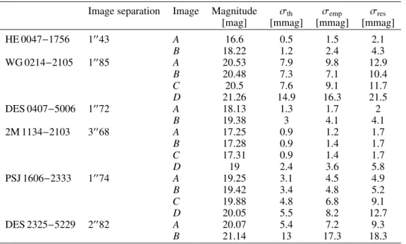
Image separation Image Magnitude σth σemp σres

[mag] [mmag] [mmag] [mmag]

HE 0047−1756 100_{43 A 16.6 0.5 1.5 2.1} B 18.22 1.2 2.4 4.3 WG 0214−2105 100_{85 A 20.53 7.9 9.8 12.9} B 20.48 7.3 7.1 10.4 C 20.5 7.6 9.1 11.7 D 21.26 14.9 16.3 21.5 DES 0407−5006 100_{72 A 18.13 1.3 1.7 2} B 19.38 3 4.1 4.1 2M 1134−2103 30068 A 17.25 0.9 1.2 1.7 B 17.28 0.9 1.4 1.7 C 17.31 0.9 1.4 1.7 D 19 2.4 3.6 5.8 PSJ 1606−2333 10074 A 19.25 3.1 4.5 4.9 B 19.42 3.4 4.8 5.2 C 19.88 4.8 6.8 9.1 D 20.05 5.5 8.2 12.7 DES 2325−5229 200_{82 A 20.07 5.4 7.2 9.3} B 21.14 13 17.3 18.3

Notes. We give the maximum image separation in Col. 2; the median observed magnitude over all the epochs in Col. 4; the expected median photon noise, σth, in Col. 5; the median empirical photon noise, σempin Col. 6 and the MAD of the residuals after fitting our intrinsic and extrinsic spline models in Col. 7. The median expected photon noise, σth, is the theoretical noise expected from the flux counts in the images whereas the empirical photon noise, σemp, corresponds to the standard deviation of the measured flux in the 4 exposures taken in the same night. σemp corresponds to the photometric uncertainties of the light curves of Fig.4.

and intrinsic variations σres(see Sect.4.1.1for details). The

lat-ter also provides an indication on the smallest intrinsic variations that can be detected by our smooth spline model. This noise esti-mate is slightly higher than σempand σthbecause it is impacted

by any fast residual variability in the data that cannot be captured by our intrinsic and extrinsic spline models.

4. Time-delay measurements

We used the public Python package PyCS6, which contains sev-eral algorithms for measuring the time delays in the presence of microlensing (Tewes et al. 2013b). We followed the procedure described in detail in Millon et al. (2020) to robustly measure time delays in an automated way. In doing this, we explored a broad range of choices for our estimator parameters and we estimated the uncertainties on the time delay using simulated light curves containing both the intrinsic and extrinsic variations. We focused on two time-delay estimators, namely the free-knot splines and the regression difference. The free-knot spline esti-mator was extensively tested on the simulated light curves of the Time Delay Challenge (Bonvin et al. 2016;Liao et al. 2015; Dobler et al. 2015) and showed very good overall performance. Throughout this paper, the error bars correspond to 1σ uncer-tainties. Negative A−B time delays means that the variations in image A lead those in image B.

4.1. Time-delay measurements with PyCS

We used the terminology defined by Bonvin et al. (2019). A curve-shifting technique is a procedure that estimates time-delay values along with their associated uncertainties given a set of light curves. This technique relies on (i) an estimator, which is an

6 _{PyCS can be downloaded fromwww.cosmograil.org}

algorithm designed to find the optimal time delay between two light curves; (ii) estimator parameters, which control the behav-ior of the estimator; and (iii) a generative noise model, which is used to produce simulated light curves, with the same constrain-ing power as the original data. The estimator is also evaluated on simulated light curves to estimate empirically the uncertain-ties. We briefly describe the two selected estimators in the fol-lowing section (seeMillon et al. 2020; Tewes et al. 2013b, for details). Estimator parameters used in this work are summarized in Table3.

4.1.1. Free-knot spline estimator

This estimator relies on the construction of an “intrinsic” model to represent the quasar variations common to all the light curves up to a time and magnitude shift and an “extrinsic” model to rep-resent the additional sources of variability that differ between the light curves. This typically includes variability introduced by the stars in the lens galaxy. Both models use free-knot B-spline to fit the light curves (Molinari et al. 2004). The algorithm simulta-neously optimizes the position of the knots of the intrinsic and extrinsic splines as well as the time delays and magnitude shifts between the light curves. The flexibility of the fit is controlled by two estimator parameters. The first, η, corresponds to the ini-tial mean spacing between knots of the intrinsic spline and the second, nml, corresponds to the number of internal nodes for the

extrinsic splines per observing season, equally distributed over the monitoring period. When we have only one season of moni-toring per object, we fix the knot position of the extrinsic splines to avoid introducing too much freedom into the microlensing models as the latter are not expected to vary on timescales shorter than a few weeks. We note that nml = 0 means that the

extrin-sic splines contain only two knots at each extremity of the light curves and therefore correspond to polynomials of degree 3.

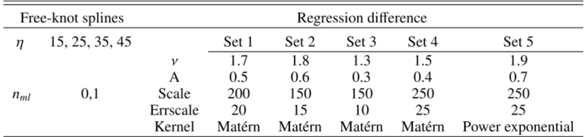
Table 3. Set of parameters used for the regression difference and free-knot spline PyCS estimator.

Free-knot splines Regression difference

η 15, 25, 35, 45 Set 1 Set 2 Set 3 Set 4 Set 5

ν 1.7 1.8 1.3 1.5 1.9

A 0.5 0.6 0.3 0.4 0.7

nml 0,1 Scale 200 150 150 250 250

Errscale 20 15 10 25 25

Kernel Matérn Matérn Matérn Matérn Power exponential

Notes. Parameter descriptions can be found in Sects.4.1.1and4.1.2.

4.1.2. Regression differences estimator

This second method first performs a regression with Gaussian processes on each light curve individually. The regressions are then shifted in time and subtracted pair-wise. The algorithm optimizes the time shift between the curves by minimizing the variability in the subtracted light curve. This approach does not explicitly model the extrinsic variations and is therefore funda-mentally different from the free-knot splines method. This esti-mator also relies on a choice of parameters to control the smooth-ness of the fit with Gaussian processes. Consequently, the kernel function of the Gaussian process, its smoothness degree, ν, its amplitude, A, its scale, and an additional scaling factor of the photometric errors need to be adjusted. We tested five different sets of parameters that visually provide a good fit of the data.

For each estimator and estimator parameters, we ran the opti-mization 500 times from different starting points (i.e., guess time delay) on the same observed light curves. This is meant to ensure that the time-delay estimator has converged and that a robust time-delay estimate can be measured independently of the initial guess for the time delay. We took the median value of the distri-bution as our central time-delay estimate. This procedure is not a Monte Carlo approach and we do not use the standard devia-tion of the distribudevia-tion as our final uncertainties. The procedure to measure the uncertainties requires the generation of simulated light curves and is summarized below.

4.2. Uncertainties estimation on the time delay with PyCS In PyCS, the uncertainties are estimated in an empirical way, by generating simulated light curves that have similar constraining power as the original data. These simulated curves are identical to the data in terms of temporal sampling, intrinsic variations of the quasar, and extrinsic variations. We used the same intrin-sic and extrinintrin-sic splines to generate all simulated light curves. However, they differ from the real data in their time delays and their realization of correlated and Gaussian photometric noise. For each set of estimator parameters, a generative noise model produces 800 different realizations of the curves that statistically match the observed data in terms of correlated and Gaussian noise. The true time delays encoded in the simulated curves are in the range ±10 days around our initial estimation obtained by running the estimator on the real data. We followed this proce-dure using the automated version of PyCS described in detail in Millon et al.(2020).

The estimators were run on the simulated light curves and we obtained the final uncertainties for a given curve-shifting tech-nique (i.e., an estimator, a set of estimator parameter, and a gen-erative noise model) by adding in quadrature the systematic and random errors between the measured and true time delays.

4.3. Combining the curve shifting techniques

To combine the curve shifting techniques and obtain our final time-delay estimates for each object, we first combined the curve-shifting techniques that share the same estimator, that is, the regression difference or the free-knot spline, which have dif-ferent sets of estimator parameters. The marginalization over the model parameters cannot be done in a fully Bayesian framework, as this would require a very large amount of computation to properly sample the parameter space. To keep the computation time manageable on a small-scale computing cluster, we pre-fer to probe the parameter space in a grid-wise fashion. The explored parameter space is limited to a region that provides rea-sonable uncertainties, indicating a good fit quality.

In addition, we cannot use the χ2_{or any derived model}

selec-tion criteria (e.g., the Bayesian informaselec-tion criterion (BIC) or the Akaike information criterion (AIC)) to estimate the weight of each model due to the degeneracy between intrinsic and extrin-sic variations. Because of this degeneracy, it is not possible to define a proper metric to quantify the quality of the fit. We there-fore prefer to apply the same methodology as first introduced inBonvin et al.(2018). The goal of this method is to obtain a trade-off between an optimization and a marginalization over the estimator parameters. A pure optimization selects the set of esti-mator parameters that gives the most precise time-delay mea-surement, but the price to pay is neglecting all the other models for the quasar variability and extrinsic variations that are not nec-essarily compatible within statistical uncertainties. On the other hand, marginalizing over all estimator parameters unnecessarily increases the uncertainties as all models are not equally plausible and do not yield the same fit quality.

To solve this problem,Bonvin et al.(2018) proposed to first select the most precise estimate as a reference and to compute its tension, τ, with all other estimates. If the tension exceeds a certain threshold τthresh = 0.5, we combine the most discrepant

estimate with the reference. This combined estimate becomes the new reference and we repeated this process until no further ten-sion exceeds τthresh. We also checked that the choice of τthreshdid

not significantly change the final estimate. We note that choosing τthresh= 0 corresponds to a marginalization between all the

avail-able sets of estimator parameters, whereas choosing τthresh= +∞

selects only the most precise set.

We obtained our final time-delay estimates for each pair of light curves and for each estimator by applying this procedure on the data. These results are presented in Figs.5–7. As the two estimators are intrinsically different but are applied to the same data set, they can not be considered as two independent measure-ments of the time delays. We therefore propose a marginalized estimate over the two curve shifting algorithms. These are shown in black in these same figures.

12

10

Delay[day]

Free-knot Spline : −

10.7

+1.2−0.9 Regression Difference : −

10.8

+0.9−0.9 Combined (

τ

thresh

= 0.0

) : −

10.8

+1.0−1.0 Free-knot Spline Regression Difference Combined (τthresh= 0.0)

HE0047

−

1756

PyCS estimates

136

134

132

130

128

126

124

122

120

Delay[day]

Free-knot Spline : −

129.4

+4.0−4.5 Regression Difference : −

127.8

+3.0−3.0 Combined (

τ

thresh

= 0.0

) : −

128.4

+3.5−3.8 Free-knot Spline Regression Difference Combined (τthresh= 0.0)

DES0407

−

5007

PyCS estimates

34

36

38

40

42

44

46

48

50

52

54

Delay[day]

Free-knot Spline :

+41.3

+3.3 −2.5 Regression Difference :

+46.6

+3.7 −3.2 Combined (

τ

thresh

= 0.0

) :

+43.8

+4.5−4.0 Free-knot Spline Regression Difference Combined (τthresh= 0.0)

DES2325

−

5229

PyCS estimates

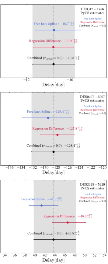
Fig. 5.Time-delay estimates for HE 0047−1756, DES 0407−5006, and DES 2325−5229 measured with the regression difference estimator (in red) and with the free-knot spline estimator (in blue). The marginaliza-tion over the two estimators is shown in black.

5. Results

The procedure described in Sect.4was applied to the six lensed quasars presented in this paper. Table 4 summarizes our mea-surements and Fig. 9 shows the relative precision on the time delays that can be achieved in one or two seasons of monitoring

and how this compares with previously published delays. All light curves presented in this work are available on the online web application D3CS7, where they can be shifted in an interac-tive way to obtain an initial guess of the time delays.

5.1. HE 0047−1756

HE 0047−1756 was monitored during one and a half seasons. At least three very prominent features can be unambiguously detected in both the A and B light curves. Our final time-delay estimate is τAB = −10.8+1.0−1.0d (9.3% precision), by combining

the two PyCS estimators. This new measurement is within the 2σ interval of a previous measurement byGiannini et al.(2017), who found τAB = −7.6 ± 1.8 d with five seasons of monitoring

at the 1.54 m Danish telescope at ESO La Silla observatory. The small discrepancy could be explained by the fact that the curve-shifting technique used in that work does not explicitly account for microlensing variation, which can possibly lead to underes-timated uncertainties. The authors also report another estimate of the time delay measured with the free-knot spline technique of PyCS τAB = −7.2 ± 3.8, which accounts for extrinsic

varia-tion. This estimate yields larger uncertainties and is compatible within 1σ with our measurement.

The time delay of HE 0047−1756 was also measured in Millon et al. (2020), who found τAB = −10.4+3.5_−3.5d using six

seasons of monitoring with the C2 camera and eight seasons with the ECAM camera successively installed on the Euler tele-scope. As the same analysis framework was applied on these last two data sets and they do not cover the same period, we can consider these experiments to be independent and therefore combine the two time-delay estimates of Millon et al. (2020) with this new campaign conducted with the WFI instrument (see Fig.8). We obtain in this way our final “PyCS-mult” estimate τAB= −10.9+0.9−0.9d (8.3% precision).

The precision of the measurement is significantly improved with high-cadence and high S/N data compared to the Euler monitoring campaigns, even though the duration of the moni-toring is much shorter. The WFI images also have on average a better seeing than the ECAM and C2 data. This allows for a better deconvolution, especially for the B component, resulting in the B light curve being of much better quality than with the Eulertelescope. Not surprisingly, this emphasizes the fact that the fainter component of each system dominates the final quality of the time-delay measurement.

5.2. WG 0214−2105

The light curves of the quadruply imaged quasar WG 0214−2105 exhibit small-scale variations on the order of 0.05−0.1 mag visible in the three brightest images, A, B, and C. These small variations happen on timescales on the order of 20 to 40 days between MHJD= 58350 and MHJD = 58450, but are not visible in the D light curve because it is too noisy. However, two larger variations of the order of 0.2 mag are also visible in all four images at the end of the first season and during the second season. These last features allow us to measure the time delays relative to image D.

The best relative precision is achieved for the BC delay, where τBC = −14.2+2.7_−2.5d (18.3% precision). The longest time

delay is between image B and image D, where τBD= −21.6+4.2_−5.0d

(21.3% precision). We can forecast how the these time-delay

7 _{https://obswww.unige.ch/~millon/d3cs/COSMOGRAIL_}

4 2 0 2 4 6 8 10 12 14 16 18

+7

.

3

+4.6 −4.6

+7.6

+1.7 −1.7

+7

.

5

+2.7 −2.9

AB

21 18 15 12 9 6 3 0 3 6

−

6

.

7

+6.2−6.2 −

6.6

+2.0−2.0 −

6

.

7

+3.6−3.6

AC

24 22 20 18 16 14 12 10 8

6

−

14

.

0

+3.9−3.9 −

14.3

+1.8−1.6 −

14

.

2

+2.7−2.5

BC

28 24 20 16 12

8

4

0

Delay[day]

−

15

.

7

+6.9−6.9 −

13.3

+3.3−3.3 −

14

.

1

+4.4−5.4

AD

36 32 28 24 20 16 12

8

Delay[day]

−

23

.

0

+6.5−6.5 −

21.0

+3.1−3.1 −

21

.

6

+4.2−5.0

BD

24 20 16 12

8

4

0

4

8

Delay[day]

−

9

.

0

+6.6−6.6 −

6.8

+3.1−3.1 −

7

.

5

+4.3−5.1

CD

Free-knot Spline Regression Difference Combined (

τ

thresh= 0

.

0)

WG0214

−

2105

PyCS estimates

Fig. 6.Same as Fig.5for WG 0214−2105.

uncertainties transfer to the H0inference if the time-delay

mea-surement remains the dominant source of errors compared to modeling and line of sight errors. This is likely to be the case here since the line of sight and modeling errors are typically on the order of 5% (seeWong et al. 2019, for the error budget of the H0LiCOW lenses). Assuming Gaussian probability distribution, we estimate that the relative uncertainty that directly propagates into the Hubble constant is on the order of ∼13.0% by combining the three time delays relative to image B independently8.

In spite of the very good agreement between the two PyCS estimators, the free-knot spline estimator yields significantly larger uncertainties than the regression difference. This might be because the free-knot spline estimator is more sensitive to the photometric noise than the regression difference, but the latter requires more inflection points in the light curves to obtain pre-cise time-delay estimates. WG 0214−2105 has relatively noisy light curves compared to other objects, but the quasar is highly variable; this might explain the good performance of the regres-sion difference. Other objects with high photometric preci-sion, but only a few inflection points in the light curves, such as PSJ 1606−2333 and 2M 1134−2103, exhibit the opposite behavior, that is, the free-knot spline estimator yields the best precision.

WG 0214−2105 was monitored for two seasons because the first season alone was not sufficient to measure any time delays at a precision better than 30% despite intrinsic variations being

8 _{The residual covariance between the three independent time delays} is expected to be small and is therefore ignored in the computation of the total time-delay error propagating to H0. We only aim to provide a rough estimate of the constraining power of each system on H0.

clearly visible. The need of a second season for this object is explained by (i) WG 0214−2105 is relatively faint so the photometric precision achieved in 30 min of exposure is lower than for other brighter objects (see Table2 for description of the photometric noise); (ii) WG 0214−2105 is a compact quad (largest image separation is 10085), which makes it more sen-sitive to deconvolution errors, again increasing the photometric noise in the light curves; and (iii) WG 0214−2105 has short time delays making it harder to obtain a good relative precision mea-surements. A third season of monitoring might be necessary to improve the time-delay precision and to make this system more valuable for time-delay cosmography. Still, this would be three times faster than with the previous COSMOGRAIL cadence and S/N on a 1 m-class telescope. Ideally, we aim for a precision below 5% on the time-delay measurement, which is the thresh-old where the time-delay error becomes subdominant compared to the modeling and line-of-sight errors (Suyu et al. 2014,2017; Wong et al. 2019).

5.3. DES 0407−5006

Only one feature is visible in the B light curve of DES 0407−5006 around MHJD= 58500 d. This feature can be matched with the drop in the A light curve around MHJD= 58370 d. Using PyCS, we obtained a final time-delay estimate of τBD = −128.4+3.5−3.8d

(2.8% precision). The long time delay of this system allowed us to reach a good relative precision although the overlap between the curves is limited. This object already has a sufficiently precise time-delay measurement to use it for time-delay cosmography. Although doubly imaged quasars are less effective, in principle,

36

34

32

30

28

26

24

−

30

.

3

+1.8−2.0 −

30.7

+2.6−2.6 −

30

.

5

+2.2−2.3

AB

4

6

8

10

12

+8

.

7

+1.1 −1.1

+8.3

+1.8 −2.0

+8

.

6

+1.4 −1.5

AC

32

34

36

38

40

42

44

+39

.

0

+1.7 −1.7

+38.9

+2.7 −2.9

+38

.

9

+2.2 −2.2

BC

90 85 80 75 70 65 60 55

Delay[day]

−

69

.

5

+3.8−5.2 −

76.3

+8.7−8.2 −

71

.

9

+5.9−8.5

AD

60 55 50 45 40 35 30 25 20

Delay[day]

−

38

.

9

+4.3−6.7 −

45.6

+9.0−8.8 −

41

.

5

+7.0−8.8

BD

100 95 90 85 80 75 70 65 60

Delay[day]

−

78

.

2

+4.2−5.4 −

84.6

+8.8−8.2 −

80

.

5

+6.2−8.4

CD

Free-knot Spline Regression Difference Combined (

τ

thresh= 0

.

0)

2M1134

−

2103

PyCS estimates

16

14

12

10

8

6

4

−

10

.

6

+1.7

−

1.9

−

10.0

+3.2

−

2.1

−

10

.

4

+2.3

−

2.2

AB

42 39 36 33 30 27 24 21 18 15

Delay[day]

−

28

.

2

+4.7

−

2.6

−

30.7

+5.6

−

6.0

−

29

.

2

+4.4

−

5.1

AC

30

27

24

21

18

15

12

9

Delay[day]

−

17

.

6

+4.4

−

2.6

−

21.5

+4.9

−

4.6

−

19

.

3

+4.2

−

4.9

BC

Free-knot Spline

Regression Difference

Combined (

τ

thresh

= 0

.

0

)

PS1606

−

2333

PyCS estimates

22 20 18 16 14 12 10 8

6

4

2 0

Delay[day]

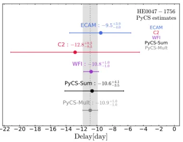
ECAM :

−9.5+3.9−4.0

C2 :

−12.8+8.3 −8.3

WFI :

−10.8+1.0−1.0

PyCS-Sum :

−10.6+4.1−3.5

PyCS-Mult :

−10.9+1.0 −1.0 ECAM C2 WFI PyCS-Sum PyCS-Mult

HE0047

−

1756

PyCS estimates

Fig. 8.Time-delay estimate of HE 0047−1756. Each point corresponds to the results of PyCS applied on a different data set. The “PyCS-sum” (in black) and the “PyCS-mult” (in shaded gray) are two possible com-binations of the results of this work with the C2 and ECAM results measured inMillon et al.(2020). “PyCS-mult” corresponds to the mul-tiplication of the probability distribution, whereas “PyCS-sum” is their marginalization.

in constraining lens models, deep high-resolution images may reveal prominent and constraining rings due to the lensed host galaxy of the quasar as inBirrer et al.(2019).

5.4. 2M 1134−2103

2M 1134−2103 is a very bright quadruply imaged quasar dis-covered byLucey et al. (2018). The monitoring started shortly after the announcement of the discovery. Very small variations on the order of ∼40 mmag (peak-to-peak) are clearly visible in all light curves. The S/N in the light curves is sufficient to record even smaller variations on the order of ∼10 mmag in the three brightest multiple images A, B, and C.

The most precise time delay is the B−C delay where τBC =

+38.9+2.2

−2.2d (5.7% precision). We also measured at least one time

delay relative to image A and image B with a precision bet-ter than 10%, τAB = −30.5+2.2_−2.3d (7.4% precision) and τCD =

−80.5+6.2_−8.4d (9.1% precision). Combining the three independent delays relative to image B and assuming Gaussian probabil-ity distribution, the total time-delay error that propagates to the Hubble constant is ∼4.4%, making this object a promising target for future time-delay cosmography analysis9. However, the lens redshift in 2M 1134−2103 is yet unknown and might be difficult to measure from the ground owing to the high contrast between the bright quasar images and the faint lens galaxy.

5.5. PSJ 1606−2333

PSJ 1606−2333 does not show fast varying features, even in the A light curve, which has the best S/N. However, slow varia-tions over the monitoring season allow us to obtain time-delay estimates with a precision below 30% for the three brightest images. We measured τAB = −10.4+2.3_−2.2d, τAC = −29.2+4.4_−5.1d,

9 _{The time-delay error might not the dominant source of errors at this} level of precision so the Gaussian approximation might not be sufficient for this object. Therefore, the total time-delay error given in this work is only an approximation.

and τBC = −19.3+4.2_−4.9, that is, a 21.6%, 16.3%, and 23.6%

pre-cision, respectively. We also measured τAD = −45.7+11.1_−10.7d, but

this time delay relative to image D is uncertain as a result of the lack of fast variation that can unambiguously be matched in all light curves. The fact that we rely on the slow variation of the quasar to measure the time delay and that the D light curve is relatively noisy makes the time-delay estimates relative to image Dmore dependent on the choice of estimator parameters and on the flexibility of microlensing model. As a consequence of this degeneracy between the slow intrinsic variation of the quasar and the slow microlensing variation, the time-delay probability distribution is multimodal, with a second peak appearing around −60 days. This second possibility however is less likely.

The combined time-delay error obtained by multiplying the two secure and independent delays relative to image A and using a Gaussian approximation is ∼13.0%. This corresponds to the error that directly propagate to H0if the time-delay error remains

the dominant source of uncertainties. These constraints are not yet sufficient for a competitive measurement of the Hubble con-stant with this system, but a second season of monitoring is likely to improve the precision given the continuous variations seen in the quasar. This will also help us better disentangle the microlensing and intrinsic variation in image D and allow us to discriminate between the two possible solutions for time delays relative to image D. The lens redshift is also unknown for this object, but the contrast between the lens and the quasar images is much lower than in 2M 1134−2103, so that a redshift determi-nation should be easier.

5.6. DES 2325−5229

DES 2325−5229 presents a quasar variation with a rise of 0.2 mag in image A in only ∼70 d between MHJD= 58270 d and MHJD= 58340 d. This feature is also clearly seen in the B light curves and allows us to measure τAB= +43.8+4.5_−4.0d (9.7%

preci-sion). We note a slight tension between the regression difference and the free-knot spline estimator at a statistical significance level of 1.1σ. In the residual A−B curve, a slowly decreasing trend is visible at the beginning of the monitoring season, which might be attributed to microlensing in one of the two multiple images. As the regression difference estimator does not explic-itly account for extrinsic variation whereas the free knot-spline estimator does, the small discrepancy between the two estima-tors could be explained by the presence of slow microlensing in the light curve.

6. Residual fast extrinsic variability

By shifting the light curves by their measured time delays and subtracting them pair-wise, we obtained difference light curves, which highlight the residual extrinsic variations. During this pro-cess, we did not correct for any microlensing variability. We observe in the B−A difference light curve of WG 0214−2105 a fast variation on the order of 0.1 mag around MHJD= 58480 and happening on a timescale of only 20 days. We observe a simi-lar effect in 2M 1134−2103, where small variations on the order of 10 mmag in the B−A difference light curve are visible at the beginning of the monitoring season.

Although these variations could be a signature of fast microlensing, the fact that this happens at the same time as an intrinsic variation that is visible in all multiple images might also indicate that an additive flux component is contaminating one or both images. To verify that an additive flux component

Table 4. Measured time delays, in days, for the two PyCS estimators and their combination (see text).

PyCS free-knot splines PyCS regression differences PyCS combined HE 0047−1756 τAB= −10.7+1.2_−0.9 τAB= −10.8+0.9_−0.9 τAB= −10.8+1.0_−1.0 WG 0214−2105 τAB= 7.3+4.6−4.6 τAB= 7.6+1.7−1.7 τAB= 7.5+2.7−2.9 τAC= −6.7+6.2_−6.2 τAC= −6.6+2.0_−2.0 τAC= −6.7+3.6_−3.6 τAD= −15.7+6.9−6.9 τAD= −13.3+3.3−3.3 τAD= −14.1+4.4−5.4 τBC = −14.0+3.9_−3.9 τBC = −14.3+1.8_−1.6 τBC = −14.2+2.7_−2.5 τBD= −23.0+6.5_−6.5 τBD= −21.0+3.1_−3.1 τBD= −21.6+4.2_−5.0 τCD= −9.0+6.6_−6.6 τCD= −6.8+3.1−3.1 τCD= −7.5+4.3_−5.1 DES 0407−5006 τAB= −129.4+4.0_−4.5 τAB= −127.8+3.0_−3.0 τAB= −128.4+3.5_−3.8 2M 1134−2103 τAB= −30.3+1.8−2.0 τAB= −30.7+2.6−2.6 τAB= −30.5+2.2−2.3 τAC= 8.7+1.1_−1.1 τAC= 8.3+1.8_−2.0 τAC= 8.6+1.4_−1.5 τAD= −69.5+3.8_−5.2 τAD= −76.3+8.7_−8.2 τAD= −71.9+5.9_−8.5 τBC= 39.0+1.7−1.7 τBC= 38.9+2.7−2.9 τBC= 38.9+2.2−2.2 τBD= −38.9+4.3_−6.7 τBD= −45.6+9.0_−8.8 τBD= −41.5+7.0_−8.8 τCD= −78.2+4.2_−5.4 τCD= −84.6+8.8_−8.2 τCD= −80.5+6.2_−8.4 PSJ 1606−2333 τAB= −10.6+1.7−1.9 τAB= −10.0+3.2−2.1 τAB= −10.4+2.3−2.2 τAC = −28.2+4.7_−2.6 τAC = −30.7+5.6_−6.0 τAD= −29.2+4.4_−5.1 τBC = −17.6+4.4_−2.6 τBC = −21.5+4.9_−4.6 τBC = −19.3+4.2_−4.9 DES 2325−5229 τAB= +41.3+3.3−2.5 τAB= +46.6+3.7−3.2 τAB= +43.8+4.5−4.0

Notes. In the case of HE 0047−1756, the final PyCS-mult estimate is τAB = −10.9+0.9−0.9d and is obtained by combining our WFI data set with monitoring data from the Leonhard Euler 1.2 m Swiss telescope (Millon et al. 2020).

does not impact the measured time delays, we fit an additional parameter corresponding to a constant shift in flux of the light curves. In practice, this corresponds to a stretch in magnitude, i.e. along the y-axis in Fig.4. This flux shift differs from a shift in magnitude that we normally apply to the light curves and that corresponds to the multiplicative (flux) factor produced by the lensing magnification.

We applied this flux correction to 2M 1134−2103 and WG 0214−2105, which are the two objects the most affected by this effect. This reduces the amplitude of the variations seen in the difference curves but does not remove them completely. Still, we applied our time-delay measurement pipeline to the corrected data. This only changes the measured time delay marginally and none of the measured time delays are shifted by more than the reported uncertainties. The maximal changes over the six measured time delays for each object corresponds to 0.4σ for WG 0214−2105 and 0.7σ for 2M 1134−2103. We thus conclude that the distortions of the light curves that we observe in these two lens systems do not significantly impact the measured time delays.

Although instrumental effects or residual contamination after the deconvolution could be a possible explanation for the observed distortion of the light curves, this might also come from the regions of multiple source sizes contributing to the R-band flux and being differently microlensed. Indeed, each lensed image is composed of a variable component (central accretion disk) and a nonvariable component; that is, the broad line region (BLR) and the central part of the bulge of the host galaxy. The latter is little or not affected at all by microlensing because its size is much larger than microcaustics. Thus, if microlensing affects the variable part of one image but not the other, this would produce variations of larger amplitude in the microlensed image and hence result in residuals in the difference light curve. A description of a similar “differential amplification” effect can

be found in Sect. 3.3.3 ofSluse et al.(2006). The lens light could also contribute to the nonmicrolensed component that is needed to produce the effect. Finally, we note that the nonmicrolensed component might also be variable as a result of the reverber-ation of the continuum emission in the BLR as suggested by Sluse & Tewes(2014).

Our new high-quality light curves probably point to new sub-tle differential microlensing effects that were unseen with data of lower quality. In the present paper, we limit ourselves to check-ing whether these effects impact time-delay cosmography, and we show that they do not. However, our data may allow us to study quasar structure on very small physical scales and at cos-mological distances. This is beyond the scope of this paper but we point to a potential opportunity to use high-cadence and high S/N multiband light curves to scrutinize the inner regions of quasars and their host galaxies with microlensing.

7. Conclusions

We present the results of the first intensive high-cadence and high S/N monitoring campaign in the framework of the TDCOSMO collaboration. We measured new time delays in three doubly imaged and three quadruply imaged quasars using data taken almost daily with the MPIA 2.2 m telescope at ESO observatory, La Silla. The most precise delay is obtained for DES 0407−5006, where τAB = −128.4+3.5_−3.8d (2.8% precision).

All other objects have at least one time delay measured with a precision better than 18.3%, including systematics due to the residual extrinsic variability. PSJ 1606−2333 presents the most uncertain estimates owing to the absence of fast intrinsic varia-tion. For this object, a second season of monitoring will be nec-essary in order to reach uncertainties on the order of ∼10% on the best measured time delay.

10% 20% 30% 40% 50%

HE

0047

−

1746

WG

0214

−

2105

DES

0407

− 5006

2M

1134

−

2103

PSJ

1606

−

2333

DES

2325

− 5229

Double from this work

Quad from this work

Delays from previous publication

0 20 40 60 80 100 Longest time dela y [da y]

Fig. 9.Time-delays relative uncertainties for the object presented in this work (colored dots) and already available in the literature (gray dots) (see Table 3 ofMillon et al. 2020, for a list of published time delays). For quadruply imaged quasars, the combined uncertainties between all three independent time delays, corresponding to the minimal uncertainties achievable on H0, are shown under the assumption that the time-delay errors remain the dominant source of uncertainties. The outer light blue circle corresponds to a precision better than 15%. The inner blue circle corresponds to the target region with precision better than 5%, corresponding to the threshold at which the time-delay errors become smaller than other sources of errors in the inference of H0.

We confirm that high-cadence and high S/N monitoring data with 2 m-class telescopes can provide precise time delay in one single season, as was first explored byCourbin et al.(2018). This observation strategy allows us to better disentangle microlens-ing from the intrinsic signal of the quasar by recordmicrolens-ing its small-amplitude and fast variations. The unprecedented qual-ity of the data also allows us to detect small distortions of the light curves between the multiple images, which are not only shifted in time and in magnitude but also stretched along the magnitude axis. This effect is detected in two lensed systems, namely 2M 1134−2103 and WG 0214−2105. We suggest that a source size effect might explain this distortion if the broadband emission contains flux arising from the compact active galactic nucleus continuum and from a spatially more extended region, such as the BLR or the bulge of the host galaxy. The di fferen-tial microlensing between those two sources of emission may explain the observed signal. Although the exact origin of this effect remains to be clarified, we can still correct for the contam-inating component and find that this does not change the mea-sured time delays.

We used two time-delay estimators in the PyCS package, namely the regression difference and the free-knot spline. We note a very good agreement between these two estimators over-all, which indicates that the choice in the modeling of the extrin-sic variability does not significantly impact the final time-delay estimates. When available, we also include monitoring data from the Leonhard Euler 1.2 m Swiss telescope from Millon et al. (2020). We combined the measurements to obtain the time delay of HE 0047−1756, τAB= −10.9+0.9_−0.9d with 8.3% precision.

As the number of known lensed quasar is increasing quickly with new wide-field surveys, the rapid follow-up of the newly discovered quasars is crucial to turn the corresponding new time delays into cosmological constraints. The Rubin Observatory Legacy Survey of Space and Time (LSST) will provide high S/N monitoring data for a large part of the sky but its cadence will be limited to one point every few days in any given band. Our observations emphasize that the highest possible temporal sampling is just as important as S/N to overcome the microlens-ing variability. It is therefore likely that LSST light curves will require complementary data from 2 m-class telescopes or larger with a daily cadence.

Acknowledgements. We warmly thank R. Gredel, H.-W. Rix and T. Henning for allowing us to observe with the MPIA 2.2 m telescope and for ensuring the daily cadence of the observations is achieved. This program is supported by the Swiss National Science Foundation (SNSF) and by the European Research Council (ERC) under the European Union’s Horizon 2020 research and innovation pro-gram (COSMICLENS: grant agreement No 787886). TT and CDF acknowledge support by NSF through grant Collaborative Research: Toward a 1% Measure-ment of The Hubble Constant with Gravitational Time Delays AST-1906976. CDF acknowledges support for this work from the National Science Foundation under Grant No. AST-1907396. SHS and DCYC thank the Max Planck Society for support through the Max Planck Research Group for SHS. T.A. acnkowledges support from Proyecto Fondecyt N 1190335 and the Ministry for the Econ-omy, Development, and Tourism’s Programa Inicativa Científica Milenio through grant IC 12009. This research made use of Astropy, a community-developed core Python package for Astronomy (Astropy Collaboration 2013,2018) and the 2D graphics environment Matplotlib (Hunter 2007).

References

Agnello, A., & Spiniello, C. 2019,MNRAS, 489, 2525

Anguita, T., Schechter, P. L., Kuropatkin, N., et al. 2018,MNRAS, 480, 5017 Astropy Collaboration (Robitaille, T. P., et al.) 2013,A&A, 558, A33 Astropy Collaboration (Price-Whelan, A. M., et al.) 2018,AJ, 156, 123 Bertin, E., & Arnouts, S. 1996,A&AS, 117, 393

Birrer, S., Treu, T., Rusu, C. E., et al. 2019,MNRAS, 484, 4726 Bonvin, V., Tewes, M., Courbin, F., et al. 2016,A&A, 585, A88 Bonvin, V., Courbin, F., Suyu, S. H., et al. 2017,MNRAS, 465, 4914 Bonvin, V., Chan, J. H. H., Millon, M., et al. 2018,A&A, 616, A183 Bonvin, V., Millon, M., Chan, J. H. H., et al. 2019,A&A, 629, A97

Cantale, N., Courbin, F., Tewes, M., Jablonka, P., & Meylan, G. 2016,A&A, 589, A81

Chambers, K. C., Magnier, E. A., Metcalfe, N., et al. 2016, ArXiv e-prints [arXiv:1612.05560]

Chen, G. C. F., Fassnacht, C. D., Suyu, S. H., et al. 2019,MNRAS, 490, 1743 Courbin, F., Bonvin, V., Buckley-Geer, E., et al. 2018,A&A, 609, A71 Dobler, G., Fassnacht, C. D., Treu, T., et al. 2015,ApJ, 799, 168

Drlica-Wagner, A., Sevilla-Noarbe, I., Rykoff, E. S., et al. 2018,ApJS, 235, 33 Eulaers, E., Tewes, M., Magain, P., et al. 2013,A&A, 553, A121

Freedman, W. L., Madore, B. F., Hoyt, T., et al. 2020,ApJ, 891, 57 Giannini, E., Schmidt, R. W., Wambsganss, J., et al. 2017,A&A, 597, A49 Hunter, J. D. 2007,Comput. Sci. Eng., 9, 90

Lemon, C. A., Auger, M. W., McMahon, R. G., & Ostrovski, F. 2018,MNRAS, 479, 5060

Lemon, C. A., Auger, M. W., & McMahon, R. G. 2019,MNRAS, 483, 4242 Liao, K., Treu, T., Marshall, P., et al. 2015,ApJ, 800, 11

Lucey, J. R., Schechter, P. L., Smith, R. J., & Anguita, T. 2018,MNRAS, 476, 927

Magain, P., Courbin, F., & Sohy, S. 1998,ApJ, 494, 472

McCully, C., Keeton, C. R., Wong, K. C., & Zabludoff, A. I. 2017,ApJ, 836, 141

Millon, M., Courbin, F., Bonvin, V., et al. 2020,A&A, 640, A105

Molinari, N., Durand, J.-F., & Sabatier, R. 2004,Comput. Stat. Data Anal., 45, 159

Mosquera, A. M., & Kochanek, C. S. 2011,ApJ, 738, 96

Ostrovski, F., McMahon, R. G., Connolly, A. J., et al. 2017,MNRAS, 465, 4325

Planck Collaboration VI. 2020,A&A, 641, A6

Rathna Kumar, S., Tewes, M., Stalin, C. S., et al. 2013,A&A, 557, A44 Refsdal, S. 1964,MNRAS, 128, 307

Riess, A. G. 2019,Nat. Rev. Phys., 2, 10

Riess, A. G., Casertano, S., Yuan, W., Macri, L. M., & Scolnic, D. 2019,ApJ, 876, 85

Rusu, C. E., Fassnacht, C. D., Sluse, D., et al. 2017,MNRAS, 467, 4220 Rusu, C. E., Wong, K. C., Bonvin, V., et al. 2019,MNRAS, 498, 1440 Shalyapin, V. N., & Goicoechea, L. J. 2017,ApJ, 836, 14

Shalyapin, V. N., & Goicoechea, L. J. 2019,ApJ, 873, 117 Sluse, D., & Tewes, M. 2014,A&A, 571, A60

Sluse, D., Claeskens, J. F., Altieri, B., et al. 2006,A&A, 449, 539 Suyu, S. H., Marshall, P. J., Auger, M. W., et al. 2010,ApJ, 711, 201 Suyu, S. H., Treu, T., Hilbert, S., et al. 2014,ApJ, 788, L35 Suyu, S. H., Bonvin, V., Courbin, F., et al. 2017,MNRAS, 468, 2590 Tewes, M., Courbin, F., Meylan, G., et al. 2013a,A&A, 556, A22 Tewes, M., Courbin, F., & Meylan, G. 2013b,A&A, 553, A120 Tihhonova, O., Courbin, F., Harvey, D., et al. 2018,MNRAS, 477, 5657 Verde, L., Treu, T., & Riess, A. G. 2019,Nat. Astron., 3, 891

Wisotzki, L., Schechter, P. L., Chen, H. W., et al. 2004,A&A, 419, L31 Wong, K. C., Suyu, S. H., Auger, M. W., et al. 2017,MNRAS, 465, 4895 Wong, K. C., Suyu, S. H., Chen, G. C. F., et al. 2019,MNRAS, 498, 1420

1 _{Institute of Physics, Laboratory of Astrophysics, Ecole} Polytech-nique Fédérale de Lausanne (EPFL), Observatoire de Sauverny, 1290 Versoix, Switzerland

e-mail: martin.millon@epfl.ch

2 _{Fermi National Accelerator Laboratory, PO Box 500, Batavia, IL} 60510, USA

3 _{Department of Physics, University of California, Davis, CA 95616,} USA

4 _{Kavli Institute for Cosmological Physics, University of Chicago,} Chicago, IL 60637, USA

5 _{Kavli Institute for Particle Astrophysics and Cosmology, Stanford} University, 452 Lomita Mall, Stanford, CA 94035, USA

6 _{Max Planck Institute for Astrophysics, Karl-Schwarzschild-Strasse} 1, 85740 Garching, Germany

7 _{Physik-Department, Technische Universität München,} James-Franck-Straße 1, 85748 Garching, Germany

8 _{Institute of Astronomy and Astrophysics, Academia Sinica, PO Box} 23-141, Taipei 10617, Taiwan

9 _{Department of Physics and Astronomy, University of California,} Los Angeles, CA 90095, USA

10 _{Departamento de Ciencias Físicas, Universidad Andres Bello} Fer-nandez Concha 700, Las Condes, Santiago, Chile

11 _{Millennium Institute of Astrophysics, Chile}

12 _{Instituto de Física y Astronomía, Universidad de Valparaíso, Avda.} Gran Bretaña 1111, Playa Ancha, Valparaíso 2360102, Chile 13 _{DARK, Niels Bohr Institute, University of Copenhagen, Lyngbyvej}

2, 2100 Copenhagen, Denmark

14 _{Centre for Extragalactic Astronomy, Department of Physics,} Durham University, Durham DH1 3LE, UK

15 _{Centro de Astroingeniería, Facultad de Física, Pontificia} Universi-dad Católica de Chile, Av. Vicuña Mackenna 4860, Macul 7820436, Santiago, Chile

16 _{Max-Planck-Institut für Astronomie, Königstuhl 17, 69117} Heidelberg, Germany

17 _{STAR Institute, Quartier Agora, Allée du six Août, 19c, 4000 Liège,} Belgium

18 _{Las Cumbres Observatory Global Telescope, 6740 Cortona Dr.,} Suite 102, Goleta, CA 93111, USA

19 _{Department of Physics, University of California, Santa Barbara, CA} 93106-9530, USA