HAL Id: hal-01440047
https://hal.archives-ouvertes.fr/hal-01440047
Submitted on 18 Jan 2017
HAL is a multi-disciplinary open access
archive for the deposit and dissemination of sci-entific research documents, whether they are pub-lished or not. The documents may come from teaching and research institutions in France or abroad, or from public or private research centers.
L’archive ouverte pluridisciplinaire HAL, est destinée au dépôt et à la diffusion de documents scientifiques de niveau recherche, publiés ou non, émanant des établissements d’enseignement et de recherche français ou étrangers, des laboratoires publics ou privés.
thermoelectric power generators
Khaled Chahine, Mohamad Ramadan, Zaher Merhi, Hadi Jaber, Mahmoud
Khaled
To cite this version:
Khaled Chahine, Mohamad Ramadan, Zaher Merhi, Hadi Jaber, Mahmoud Khaled. Parametric analysis of temperature gradient across thermoelectric power generators. Journal of Electrical Systems, ESR Groups, 2016, 12 (3), pp.623-632. �hal-01440047�
* Corresponding author: K. Chahine, Electrical and Electronics Engineering Department, Lebanese International
University, PO Box 146404 Beirut, Lebanon, E-mail: [email protected]
1
Energy and Thermo-Fluids Group ETF, School of Engineering, Lebanese International University, PO Box 146404 Beirut, Lebanon
2
Laboratoire de Génie Industriel, CentraleSupélec, 92290 Châtenay-Malabry, France
3
Univ Paris Diderot, Sorbonne Paris Cité, Institut des Energies de Demain, Paris-France
Copyright © JES 2016 on-line : journal/esrgroups.org/jes
Khaled Chahine1, *, Mohamad Ramadan1, Zaher Merhi1, Hadi Jaber2, Mahmoud Khaled1, 3 J. Electrical Systems 12-3 (2016): 623-632 Regular paper
Parametric analysis of temperature gradient across thermoelectric power
generators
J
E
S
Journal of Journal of Journal of Journal of Electrical Electrical Electrical Electrical Systems Systems Systems SystemsThis paper presents a parametric analysis of power generation from thermoelectric generators (TEGs). The aim of the parametric analysis is to provide recommendations with respect to the applications of TEGs. To proceed, the one-dimensional steady-state solution of the heat diffusion equation is considered with various boundary conditions representing real encountered cases. Four configurations are tested. The first configuration corresponds to the TEG heated with constant temperature at its lower surface and cooled with a fluid at its upper surface. The second configuration corresponds to the TEG heated with constant heat flux at its lower surface and cooled with a fluid at its upper surface. The third configuration corresponds to the TEG heated with constant heat flux at its lower surface and cooled by a constant temperature at its upper surface. The fourth configuration corresponds to the TEG heated by a fluid at its lower surface and cooled by a fluid at its upper surface. It was shown that the most promising configuration is the fourth one and temperature differences up to 70˚C can be achieved at 150˚C heat source. Finally, a new concept is implemented based on configuration four and tested experimentally.
Keywords: Energy harvesting; thermoelectric generation; Seebeck effect; waste heat recovery.
Article history: Received 28 March 2016, Accepted 16 August 2016
1. Introduction
The adverse climate changes being witnessed across the planet together with the ever-decreasing reserves of primary resources, resulting from rapid growth in energy demand due to population growth and industrialization, have raised public awareness to the dire consequences of pollution and inefficient energy usage. Indeed, promoting energy efficiency [1], energy-saving behaviors and renewable energy systems [2-5] has become an essential part of the energy policies and strategies in developed countries. In 2007, the European Council set the following ambitious targets to be achieved by 2020: reducing emissions of greenhouse gases by 20% with respect to the 1990 levels, improving energy efficiency with the aim of saving 20% of the European Union energy consumption, and raising the renewable energy sources share to 20% [6]. It is hence of strategic importance to optimize energy usage and explore new green energy sources.
An abundant source of energy that remains largely unharvested is waste energy [7], and especially waste heat [8-10]. Almost one-third of the energy consumed by industry is released as thermal losses directly to the atmosphere or to cooling systems [11]. These discharges result from the losses that occur in engineering systems. This waste heat can be recovered into a useful source of energy.
Thermoelectric materials allow converting a temperature gradient into electricity. Although they are not yet efficient enough to be applied industrially on large scale, TEGs present the advantages of being silent, scalable and reliable [12, 13]. Therefore, a deeper understanding of the parameters that affect the thermoelectric performance of TEGs is required for reaching adequate conversion levels.
The present work concerns heat transfer modeling and parametric analysis of the thermal behaviors of TEG subjected to different boundary conditions. The ultimate aim is to suggest new applications and/or strategies towards maximizing the temperature gradient across a TEG and hence its power output. Upon the investigation of four different configurations, each having different modes and boundary conditions, promising results were obtained regarding one configuration in which the temperature gradient is formed between two convection boundaries. A new concept is then implemented based on the promising configuration and tested experimentally.
The remaining of the paper is organized as follows: section 2 presents the parametric analysis for the different configurations, section 3 shows the experimental results, and finally section 4 draws the conclusions.
2. Parametric analysis and recommendations
This section concerns a parametric analysis of the TEG thermal behavior subjected to several conditions. The aim is to find recommendations as to obtaining significant temperature gradient through the TEG module.
Although a temperature gradient is the trigger for a TEG to generate power, practically this gradient is not exactly nor necessarily obtained by fixing the temperatures at the two TEG surfaces. Moreover, fixing the temperatures at the two surfaces of the TEG requires external means requiring power. The most common boundary conditions that are encountered in practice will be exposed and treated below. For each case, the temperature gradient between the hot and cold surfaces of the TEG will be evaluated at steady state and parametrically analyzed.
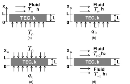
Figure 1 shows schematics of the different configurations that will be tested.
TEG, k L Fluid 0 L x ∞
T
0T
(a) TEG, k L Fluid 0 L x ∞T
(b) TEG, k L 0 L xT
0 (a) TEG, k L Fluid 0 L x 2 ∞T
(d) '' 0q
h h '' 0q
h2 Fluid 1 ∞T
h1Fig. 1. Schematics of (a) configuration 1, (b) configuration 2, (c) configuration 3, and (d) configuration 4.
J. Electrical Systems 12-34 (2016): 623-632
625 In configuration one (Figure 1-a), the TEG of thickness L and thermal conductivity
k
is subjected to a constant temperatureT
0 at its hot side and simultaneously cooled by air having a convective coefficienth
and temperatureT
∞.In configuration two (Figure 1-b), the TEG is subjected to a constant heat flux
q
0'' at its hot side and simultaneously cooled by air having a convective coefficienth
and temperatureT
∞.In configuration three (Figure 1-c), the TEG is heated at its hot side with a constant heat flux
q
0'' and simultaneously subjected to a constant temperatureT
0 at its cold side.In configuration four (Figure 1-d), the TEG is heated at one side with air having a temperature
T
∞1 and convective heat transfer coefficienth
1 while being simultaneously cooled with air having a temperatureT
∞2and convective heat transfer coefficienth
2at the other side.For the different conditions, the TEG is considered as a plane wall and the conduction through it as one-dimensional and steady. Then, the heat diffusion equation is reduced to:
0
2 2=
dx
T
d
(1)The temperature distribution and the temperature gradient in all configurations can both be obtained by solving the differential equation of the heat diffusion equation above, but will vary according to the boundary conditions. In all of the above configurations, integrating the reduced form of the heat diffusion equation with respect to
x
yields the below linearvariation dependent on two constants
A
andB
function of the boundary conditions:( )
x
Ax
B
T
=
+
(2) Below, the boundary conditions, temperature distributions and temperature differences corresponding to the four configurations are exposed.Configuration 1
(
0
,
t
)
T
0T
=
(3-a)(
)
[
∞]
=−
=
−
h
T
L
t
T
dx
dT
k
L x,
(3-b)( )
(
)
0 0T
x
hL
K
T
T
h
x
T
+
+
−
=
∞ (3-c)(
)
hL
k
T
T
hL
T
+
−
=
∆
0 ∞ (3-d) Configuration 2 '' 0 0q
dx
dT
k
x=
−
= (4-a)(
)
[
∞]
=−
=
−
h
T
L
t
T
dx
dT
k
L x,
(4-b)( )
'' 0 '' 0q
hk
k
hL
T
x
k
q
x
T
=
−
+
∞+
+
(4-c)k
L
q
T
'' 0=
∆
(4-d) Configuration 3 '' 0 0q
dx
dT
k
x=
−
= (5-a)(
L
,
t
)
T
0T
=
(5-b)( )
L
k
q
T
x
k
q
x
T
'' 0 0 '' 0+
+
−
=
(5-c)k
L
q
T
'' 0=
∆
(5-d) Configuration 4( )
(
10
)
1 0T
T
h
dx
dT
k
x−
=
−
∞ = (6-a)( )
(
2)
2 ∞ =−
=
−
h
T
L
T
dx
dT
k
L x (6-b)( )
(
)
(
)
(
)
(
h
h
)
h
h
L
k
T
T
kh
T
x
L
h
h
h
h
k
T
T
h
h
x
T
2 1 2 1 1 2 2 1 2 1 2 1 1 2 2 1+
+
−
+
+
+
+
−
=
∞ ∞ ∞ ∞ ∞ (6-c)(
)
(
h
h
)
h
h
L
L
k
T
T
k
h
h
T
2 1 2 1 2 1 2 1+
+
−
=
∆
∞ ∞ (6-d)J. Electrical Systems 12-34 (2016): 623-632
627
From equation 3-d, it is obvious that the higher the temperature prescribed at one surface of the TEG
T
0, the lower the fluid temperatureT
∞, and the lower the thermal conductivity of the TEG, the higher will be the temperature gradient. On the other hand, no direct conclusions can be made with respect to the thicknessL
and convective coefficienth
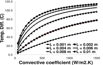
. To proceed and have clear magnitude orders and recommendations, a parametric analysis with respect to the mentioned parameters is carried out. Figure 2 shows the variation of the temperature gradient through the TEG in function of the convective coefficienth
for different thicknessL
of the TEG. For the set of calculations corresponding to Figure 2, the temperature at the hot surfaceT
0 is fixed at 150°C, the fluid temperatureT
∞ at 20°C, and the thermal conductivity of the TEG at 2 W/m.K.From Figure 2, one can conclude that increasing the convective coefficient and thickness L will increase the temperature gradient. As illustration and magnitude orders for a thickness of 1 mm, when the convective heat transfer coefficient increases from 50 to 1500 W/m2.K, the temperature difference through the TEG increases from 3.2 to 55.7°C. For a thickness of 10 mm, the temperature difference increases from 26 to 114.7°C when the convective heat transfer coefficient increases from 50 to 1500 W/m2.K.
0.0 20.0 40.0 60.0 80.0 100.0 120.0 0 500 1000 1500
T
e
m
p
. D
if
f.
(
C
)
Convective coefficient (W/m2.K) L = 0.001 m L = 0.002 m L = 0.004 m L = 0.006 m L = 0.008 m L = 0.01 mFig. 2. Variation of the temperature gradient in function of the convective coefficient for different TEG thicknesses.
Despite having a relatively high temperature gradient in correspondence with the heat convective coefficient, this configuration only exists when the convective heat coefficient reaches very high values (values higher than 1000 W/m2.K).
Results for configurations 2 and 3
Looking at equations 4-d and 5-d of configurations 2 and 3, it is obvious that the higher the heat flux
q
0'' at one of the surfaces of the TEG, the larger the thickness of the TEGL
, and the lower the TEG thermal conductivityk
, the higher will be the temperature gradient through the TEG module.Therefore, configurations two and three are dependent on three parameters. The first is the heat flux, which in most applications is obtained from the solar radiation and can be
approximated by a constant value, thus nothing can be improved regarding it when existent as boundary condition. The two other remaining parameters which both can be improved are the thermal conductivity and the thickness of the TEG. This improvement is linked to the design of the TEG. So the optimization of the temperature gradient in configurations two and three depends on the dimensions and physical properties of the thermoelectric generator and slightly on the boundary condition (application). On the other hand, it is recommended to use TEG in configurations two and three when high heat fluxes are present. Indeed for typical values of
k
of 1 W/m.K andL
of 5 mm, temperature gradients higher than 10°C will be obtained for heat fluxes starting from 2000 W/m2.Results for configuration 4
From equation 6-d, it is obvious that the temperature gradient through the TEG increases when the temperature difference between the hot and cold fluids
T
∞1− T
∞2 increases and when the thermal conductivity of the TEG decreases. On the other hand, no direct conclusions can be made with respect to the convective coefficientsh
1andh
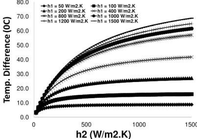
2. To proceed and have clear magnitude orders and recommendations, a parametric analysis with respect to the mentioned parameters is carried out. Figure 3 shows the variation of the temperature gradient through the TEG in function of the convective coefficienth
2 for different values of the convective coefficienth
1. For the set of calculations corresponding to Figure 3, the temperature at the hot fluidT
∞1is fixed at 150°C, the temperature of the cold fluidT
∞2 at 20°C, the thickness of the TEG module at 3 mm, and the thermal conductivity of the TEG at 2 W/m.K.0.0 10.0 20.0 30.0 40.0 50.0 60.0 70.0 80.0 0 500 1000 1500
Te
m
p
.
D
if
fe
re
n
ce
(
0
C
)
h2 (W/m2.K)
h1 = 50 W/m2.K h1 = 100 W/m2.K h1 = 200 W/m2.K h1 = 400 W/m2.K h1 = 800 W/m2.K h1 = 1000 W/m2.K h1 = 1200 W/m2.K h1 = 1500 W/m2.KFig. 3. Variation of the temperature gradient in function of the convective coefficients of the hot and cold fluids.
From Figure 3, one can conclude that increasing the convective coefficients of the hot and cold fluids increases the temperature difference across the TEG. As illustration, for a convective coefficient
h
1 of 50 W/m2.K and when the convective heat transfer coefficient2
J. Electrical Systems 12-34 (2016): 623-632
629 increases from 2.7 to 8.8°C. For a convective coefficient
h
1 of 1500 W/m2.K, the temperature difference increases from 3.7 to 68.8°C when the convective heat transfer coefficienth
2increases from 20 to 1500 W/m2.K.A remarkable feature in the curves of Figure 3 is that for many values of the convective coefficient
h
1, the temperature difference becomes almost constant or slightly varies when the convective coefficienth
2increases. This means that the choice of the two fluid flow configurations in practice should be selected taking into consideration the couple of values ofh
1 andh
2that do not correspond to the constant or slightly varying regions of the curves.Such configuration can be promising since up to relatively high values of convective heat coefficients, the temperature gradient obtained is of significant value and can be used in generating power for different applications.
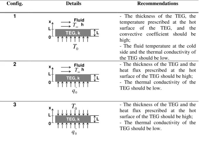
Table 1 finally summarizes the different recommendations given with each of the four configurations.
Table 1. Summary of recommendations.
Config. Details Recommendations
1 TEG, k L Fluid 0 L x ∞
T
0T
h- The thickness of the TEG, the temperature prescribed at the hot surface of the TEG, and the convective coefficient should be high;
- The fluid temperature at the cold side and the thermal conductivity of the TEG should be low.
2 TEG, k L Fluid 0 L x ∞
T
'' 0q
h- The thickness of the TEG and the heat flux prescribed at the hot surface of the TEG should be high; - The thermal conductivity of the TEG should be low.
3 TEG, k L 0 L x
T
0 '' 0q
- The thickness of the TEG and the heat flux prescribed at the hot surface of the TEG should be high; - The thermal conductivity of the TEG should be low.
4 TEG, k L Fluid 0 L x 2 ∞
T
h2 Fluid 1 ∞T
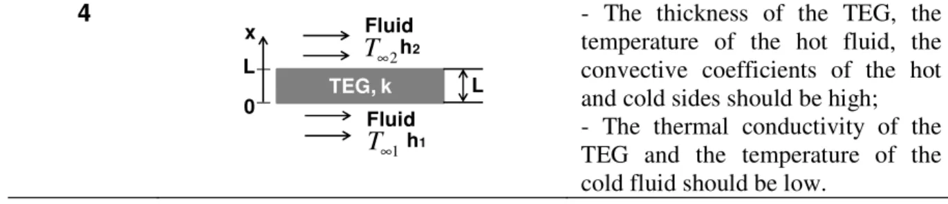
h1- The thickness of the TEG, the temperature of the hot fluid, the convective coefficients of the hot and cold sides should be high; - The thermal conductivity of the TEG and the temperature of the cold fluid should be low.
As conclusion, the most promising configuration is configuration 4 provided that the designer selects the appropriate couple of convective heat transfer coefficients since it has the most promising magnitude orders and corresponds at the same time to real configurations that can be encountered in engineering practice. All the configurations can be more promising if the thermal conductivity of the TEG can be lowered and its thickness increased which is related to the enhancement of the design of the TEG itself. Configurations 2 and 3 can be also promising if the applications involve high and extreme heat fluxes. Configuration 1 can also be more promising for applications where high temperatures are present.
The following section will be devoted to the implementation of configuration 4 in a real case and corresponding tests and thermal behaviors.
3. Experimental results
The study presented in the previous section has shown that configuration 4 presents the higher gradient of temperature for the same conditions. As an application, a system that is heated by solar energy can be suggested, where the hot fluid is heated by solar rays, whereas cold fluid is water (or other fluid) at ambient temperature. In the frame of this paper this system will be simulated experimentally by a prototype (see Figure 4).
Fig. 4. Prototype simulating TEG undergoing heating and cooling by convection It is constructed of two boxes that are separated by a layer of epoxy representing the TEG and having the same physical characteristics, that is to say the same thickness and almost the same conductivity. The boxes contain the hot and cold fluids, which are respectively oil and water. To measure the temperature difference thermo-couples are installed on the upper and lower surfaces of the epoxy layer. The tanks are insulated to decrease the heat loss with the surroundings. For simplicity, the oil is heated by an electrical heater.
J. Electrical Systems 12-34 (2016): 623-632
631 Fig. 5. Variation of temperature difference in function of time
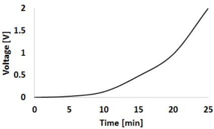
Figure 5 presents the variations of temperature at the upper and lower surfaces of the epoxy layer with time as well as the variation of the temperature gradient. The experiment is carried out over 25 minutes. The hot temperature varies from 25°C to 110°C. The cold temperature is almost constant and increases from 25°C to 30°C. The temperature difference in its turn increases with time to reach a maximum of 80°C. The electrical power that may be obtained when the TEG undergoes a temperature difference depends on the characteristics of the TEG. If a maximum power voltage of 0.025 V per 1°C of temperature difference is considered, the obtained variation of the voltage for the above-mentioned time duration is between 0 and 2 V as shown in Figure 6.
Fig. 6. Variation of voltage in function of time
4. Conclusions
A parametric analysis concerning TEG is presented. A mathematical model is proposed to simulate the thermal behavior of TEG. Several configurations were considered. It was shown that the configuration with hot and cold fluid on the top and bottom of TEG offers the highest temperature difference. An experimental study is carried out as a proof of concept. The results showed that a temperature difference of 80°C could be obtained when the hot fluid reaches 110°C and the cold fluid is initially at 25°C. The obtained voltage depends on the characteristics of utilized TEG. For such a temperature difference, an average voltage of 2V can be obtained.
References
[1] F. Z. Zerhouni, M. Zegrar, M.T Benmessaoud & A. Boudghene Stambouli, Improvement of green clean energy system’s operation, Journal of Electrical Systems, 5(2), June 2009.
[2] J. G. Fantidis, D. V. Bandekas, C. Potolias & N. Vordos, Financial and economic crisis and its consequences to the diesel-oil and biomass heating market-Case study of Greece, Journal of Electrical Systems, 8(2), 249 – 261, June 2012.
[3] A. Mohammedi, D. Rekioua & N. Mezzai, Experimental study of a PV water pumping system, Journal of Electrical Systems, 9(2), 212 – 222, June 2013.
[4] S. Slouma, S. S. Mustapha, I. S. Belkhodja & M.Orabi, An improved simple fuel cell model for energy management in residential buildings, Journal of Electrical Systems, 11(2), 145 – 159, June 2015.
[5] A. Ben Rhouma, J. Belhadj & X. Roboam, Control and energy management of a pumping system fed by hybrid Photovoltaic-Wind sources with hydraulic storage – static and dynamic analysis – U/f and F.O.C controls methods comparisons, Journal of Electrical Systems, 4(4), 1 – 16, December 2008.
[6] Brussels European Coucil, Presidency Conclusions, 8/9 March 2007.
[7] M. Ramadan, M. Khaled & H. El Hage, Using Speed Bump for Power Generation –Experimental Study, Energy Procedia, 75, 867–872, 2015.
[8] M. Khaled, M. Ramadan & H. El Hage, Parametric Analysis of Heat Recovery from Exhaust Gases of Generators, Energy Procedia, 75, 3295–3300, 2015.
[9] M. Ramadan, M. Gad El Rab & M. Khaled, Parametric analysis of air–water heat recovery concept applied to HVAC systems: Effect of mass flow rates, Case Studies in Thermal Engineering, 6, 61-68, 2015.
[10] M. Khaled, M. Ramadan, K. Chahine & A. Assi, Prototype implementation and experimental analysis of water heating using recovered waste heat of chimneys, Case Studies in Thermal Engineering, 5, 127-133, 2015.
[11] I. Johnson & W. T. Choate, Waste Heat Recovery: Technology and Opportunities in U.S. Industry, BCS, Incorporated, March 2008.
[12] L. E. Bell, Cooling, Heating, Generating Power, and Recovering Waste Heat with Thermoelectric Systems, Science, 321, 1457, 2008.