An advanced tool for Preventive Voltage Security Assessment

An Advanced Tool for Preventive Voltage Security Assessment

T. Van Cutsem

F. Capitanescu C. Moors

D. Lefebvre

V. Sermanson

University of Liège Hydro-Québec Electricité de France

Belgium Canada France

1

Department of Electrical Engineering, Sart Tilman, B28, B-4000 Liège, Belgium; vct@montefiore.ulg.ac.be

Summary. This paper deals with methods for the

preventive assessment of voltage security with respect to contingencies. We describe a computing tool for the determination of secure operation limits, together with methods for contingency filtering. Examples from two very different real-life systems are provided. We outline extensions in the field of preventive control.

Keywords. Voltage security assessment, contingency

analysis, contingency filtering, preventive control

1. INTRODUCTION

In the recent past, a significant number of incidents throughout the world have resulted in severely depressed voltage profiles or even system collapse. They have led power companies to pay much attention to voltage stability in both expansion and operational planning.

In this paper we focus on long-term voltage stability in which load restoration by Load Tap Changers (LTCs) and thermostatic effects, generator OverExcitation Limiters (OELs), shunt compensation switching and secondary voltage control play the main role [1,2]. While already a major concern in vertically integrated companies, Voltage Security Assessment (VSA) becomes even more important in the open access environment, owing to the economical incentive to operate transmission systems closer to their limits [3,4]. In this context, it is the responsibility of the transmission system operator to evaluate security margins with respect to credible contingencies and

determine the best preventive control actions to restore sufficient margins. Appropriate security criteria and efficient computer methods are needed to determine acceptable power transfer limits and identify the most appropriate generation rescheduling in case of congestion. While the linear nature of thermal limit problems allows to devise rather simple approaches, the nonlinear nature of voltage instability raises some important difficulties.

In this paper we describe the methods underlying a VSA computing tool developed at the University of Liège. Extensive tests of these methods have been performed and significant improvements have been brought within the context of our collaboration with Electricité de France and Hydro-Québec, who incorporated this tool to their operational planning software. A few examples from these two very different systems are given in the paper. Finally, we describe recent extensions and ongoing investigations in the field of voltage security analysis and control.

2. SECURITY LIMITS AND MARGINS

2.1. System stress

Our analysis of voltage security relies upon the definition of a system stress. A stress corresponds to changes in load and generation which make the system weaker by increasing power transfer over relatively long distances and/or by drawing on reactive power reserves.

The stress considered in this paper corresponds to changes in bus power injections with a single degree of freedom. Namely, at the i-th bus, the load active power Pli, the load reactive power Qli or the generator active power Pgi vary according to:

Pli = Pli o +

λ

µ

λ

where Plio, Qlio and Pgioare the corresponding base case values, S is a scaling factor, and (λli, µli, λgi) are participation factors. These factors define the "direction of stress". We assume that the direction of stress is chosen such that when S increases, voltage security decreases.

Two typical directions of stress are:

- a load increase in an area A1, covered by generation in a remote area A2. This corresponds to :

λ

µ

λ

- a generation decrease in area A1 covered by a generation increase in a remote area A2. This corresponds to :

λ

λ

We believe that in an open access environment, most transactions for which voltage security has to be checked, can be expressed in terms of the above two stresses.

2.2. Secure operation limits

For a given direction of stress and predefined contingencies, a Secure Operation Limit (SOL) corresponds to the maximum value of S, such that the system can withstand any of the specified contingencies [4].

A SOL can be easily interpreted insofar it refers to pre-contingency parameters that operators can either observe (e.g. load increase) or control (e.g. generation rescheduling within the context of a transaction).

2.3. Limit search algorithms

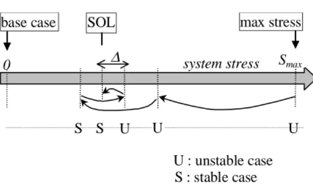
Binary search2 is a simple and robust method to determine the SOL with respect to one contingency. It consists of building an interval [Sl Su] of S values such that Sl corresponds to a stable post-contingency evolution, Suto an unstable one, and Su- Slis smaller than a specified tolerance∆. The search starts with Su set to Smax, the maximum stress of interest, and Slset to a lower bound of the sought limit. It is common (but not mandatory) to start with Sl= 0, corresponding to the current system state (or base case situation). At each step, the interval is divided in two equal parts; if the midpoint is found stable (resp. unstable) it is taken

2

also referred to as dichotomic search or bisection method

as the new lower (resp. upper) bound. The procedure is illustrated in Fig. 1, where the horizontal arrows show the sequence of tested stress levels, starting from the maximal one. U U S U : unstable case S : stable case ∆

base case SOL max stress

U S

0 system stress Smax

Figure 1: Principle of the binary search of an SOL

When the objective is to determine the SOL with respect to the most severe of a set of contingencies, it would be a waste of time to repeat the procedure of Fig. 1 for each contingency. It is more efficient to perform a Simultaneous Binary Search (SBS), in which, at a given step of the binary search, the various contingencies stemming from the previous step are simulated. If at least one of them is unstable, the stable ones are discarded since their limits are higher than the current stress level; the search proceeds with the unstable ones only. By so doing, the procedure provides for each contingency an interval containing its SOL. The width of this interval is the requested accuracy∆ for the most dangerous contingency. The more dangerous the contingency, the smaller the width of its interval. U U S U : unstable case S : stable case ∆ U S S U S U U S contin. # 1 contin. # 2 contin. # 3 S

0 S2 S4 S3 S1 system stress Smax

contin. # 4

Figure 2: Principle of the simultaneous binary search SOL

This is illustrated in Fig. 2 for a simple case with four contingencies. At maximum stress, contingency Nb. 4 is found stable and is thus already discarded. The same happens at stress S1 (resp. S3) for contingency Nb. 3 (resp. Nb. 2). The most severe contingency is the first one, and its SOL is thus the overall SOL. The SOL of contingency Nb. 3 is in the interval [S1Smax] while that of contingency Nb. 2 in [S3 S1]. The interval of the more severe contingency Nb. 2 is narrower.

The SBS converges to the most severe contingency. Of course, one may also wish to specify a level of stress below which all limits are sought (at an extra computational cost) with the ∆ accuracy. Indeed, it may be of interest to know others than the smallest limit :

- when the latter corresponds to a severe contingency with a lower probability of occurrence,

- or to a contingency whose effects are limited to a small part of the system only;

- when the system has more than one vulnerable areas and the critical contingency is to be found in each of them.

Note finally that the computational effort can be straightforwardly distributed over several computers, each dealing with one contingency.

2.4. Computing tools

Pre-contingency stress. The system operating states corresponding to various stress levels S can be computed with a standard load flow, or possibly an optimal power flow. In this calculation, it may be desirable to account for operators or controllers reacting to the system stress. These actions generally aim at keeping the voltage profile within limits and maximizing the reactive reserves readily available to face incidents. Among them, let us quote : the switching of shunt compensation, the adjustment of generator voltages or transformers tap ratios, or secondary voltage control.

Contingency evaluation. We use Quasi Steady-State (QSS) simulation in order to evaluate the impact of a contingency at a given stress level. QSS simulation combines the advantages of time-domain methods (accuracy, interpretability of results, possibility to obtain information on the instability mode, etc.) with the computational efficiency of static (mainly load flow type) methods. This fast time-domain method consists in replacing the short-term dynamics, considered infinitely fast, by equilibrium (i.e. algebraic) equations, while focusing on the long-term dynamics. The method is well documented in e.g. [2, 4-7]. It has been carefully validated with respect to multi-time-scale (i.e. full) simulation on the Hydro-Québec [6] and EDF systems.

Clearly, devices which contribute to post-contingency system stabilization must be accounted for. Usually, only automatic controls are considered since the operators' reaction in the time interval of several minutes is deemed uncertain. Time-domain methods are needed to properly account for those dynamic controls. This has early motivated Hydro-Québec and EDF to use QSS simulation.

As regards security criteria, it is common to assess the system ability to survive "credible" (e.g. N-1) contingencies with the sole help of controls that do not prevent load restoration. For instance, shunt compensation switching or secondary voltage control will be considered, but not LTC blocking, LTC voltage reduction, nor load shedding, which impact on customers. The adequacy of these stronger controls is checked against more severe disturbances.

2.5. Self-stopping QSS simulation

A system is long-term stable if, following a disturbance, the LTCs can restore their controlled voltages. Consequently, the load powers are brought back to their pre-disturbance values. Taking into account the LTC deadbands, we define the unrestored load power as :

C(t) =

Σ

Σ

-

ε

where Vi is the voltage at the i-th bus, f() represents the voltage dependence of the load active power,εi is half the LTC deadband and I denotes the set of LTC controlled load buses whose voltage is below the lower bound of that deadband, i.e. Vi < Vi0 -εi .

After a disturbance, C(t) assumes a negative value, owing to the load decrease with voltage. If the system is stable, C(t) comes back to zero after some time, since eventually I becomes empty3. In a typical unstable scenario, C(t) increases up to a (negative) maximum and then decreases. In the case of a severe disturbance it can happen that C(t) decreases right away after the disturbance. Both behaviours can be easily explained on a single-LTC system [2].

The detection of this maximum of C(t) during the QSS simulation is the basis of a self-stopping criterion, allowing to anticipate the unstable response of the system and hence to save some computing time. In order to identify this maximum, it is required to observe C(t) over a time windowτ. The simulation is stopped at a time t' such that :

∀

∈

τ

τ

Now, in marginally stable cases, C(t) may undergo oscillations or jumps before going back to zero and during this uncertain evolution, misleading local maxima are quite possible. As a safe-guard, we specify that when C(t) becomes larger than a (negative) threshold G, the simulation is continued up to the end, unless C(t) falls back below G, in which case the stopping criterion (6) is activated again.

3

On the other hand, it can also be decided to stop and declare a simulation stable once C(t) becomes larger or equal to a small (negative) value G' > G. Choosing G' = 0 amounts to stopping the simulation as soon as all LTC-controlled loads are restored within their deadbands.

2.6. Contingency filtering

When a large set of contingencies has to be processed, contingency filtering (or screening) becomes essential [6,8,9]. A filtering is performed at the first step of the SBS, when discarding those contingencies which leave the system stable at maximum stress. However, in spite of the QSS simulation speed, it may take too long to simulate the system response to each contingency of a long list. An additional pre-filtering is needed before the SBS is launched. In a majority of systems, post-contingency load flows can be advantageously used to this purpose.

Load flow equations with constant power loads and enforcement of generator reactive limits correspond to the long-term equilibrium that prevails after load voltage restoration by LTCs and machine excitation limitation by OELs. Insofar as voltage instability results from the loss of such an equilibrium [2], the corresponding load flow equations no longer have a solution and the Newton-Raphson algorithm diverges. However, using the divergence as an instability criterion meets the following difficulties :

1. divergence may result from purely numerical problems (this is particularly true when controls have to be adjusted and/or many generators switch under limit)

2. some dynamic controls that help stability cannot be accounted for in the static load flow calculation 3. conversely, some system dynamics may be responsible for an instability not detected by the load flow.

In the pre-filtering load flow, errors 1 and 2 will induce false alarms and hence some more computational effort for the SBS. Error 3, on the other hand, will mask some potentially dangerous contingencies. To reduce this second risk, a contingency is declared potentially harmful not only if the load flow diverges but also if some post-contingency voltages fall below a pre-specified threshold.

To reduce the above errors, it is essential that the load flow data match closely the model used in QSS simulation. More particularly:

- generator reactive power limits must be updated with the active power output and terminal voltage - any active power imbalance (caused by a

generator tripping or a loss of connexity) must not be left to the slack-bus but distributed over the generators according to frequency control.

To speed up the post-contingency load flows :

- divergence is early detected by monitoring the sum of squared mismatches ϕ = Σ gi2, where

g(x)=0 denotes the load flow equations. If ϕ

increases from one iteration to the next, divergence is declared and the computation stops. This test is skipped at the iteration which follows the enforcement of generator reactive limits (since ϕ increases owing to the added generator reactive power equations, not necessarily because of divergence);

- controls that marginally improve voltage stability margins are ignored;

- tolerances on mismatches are somewhat relaxed and the maximum number of iterations somewhat decreased.

2.7. Implementation

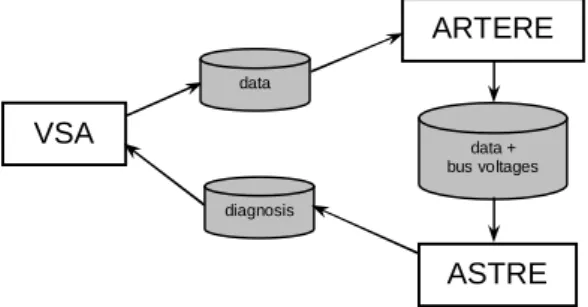
The software which implements the above algorithms is organized in three modules, which are three executables communicating through files, as sketched in Fig. 3.

Figure 3: Overall design of the program

ARTERE is a load flow program, using the full Newton-Raphson method. It is used for (i) generating stressed pre-contingency operating points, and (ii) analysing contingencies in the pre-filtering mode, with the speed-ups mentioned in the previous section. In both cases, the generator reactive limits are computed accurately, by picking up the relevant generator parameters (synchronous and leakage reactances, saturation coefficients, field current limit) in the data files shared by all the modules.

ASTRE is the QSS simulation program. It can simulate numerous contingencies, sequentially in a single execution. Criteria can be checked during and/or at the end of each simulation. ASTRE also performs the sensitivity and eigenvector computations mentioned in Section 5.

VSA calls the other two modules as needed by the previously described search algorithms. In particular, it passes to ASTRE the list of contingencies to simulate and collects the corresponding diagnoses. VSA also offers the possibility to "replay" any combination of system stress and contingency. Its graphical user

VSA ARTERE data + bus voltages ASTRE diagnosis data

interface allows to specify the direction of stress, the contingencies, the criteria, etc.

3. EXAMPLE FROM THE HYDRO-QUEBEC

SYSTEM

The Hydro-Québec system is characterized by great distances (more than 1000 km) between the large hydro generation areas (James Bay, Churchill Falls and Manic-Outardes) and the main load center (around Montréal and Québec City). Accordingly, the company has developed an extensive 735-kV transmission system, whose lines are located along two main corridors. The system is angle stability limited in the North, voltage stability limited in the South (near the load center). Frequency stability is also a concern due to the system interconnection through DC links only, as well as the sensitivity of loads to voltage.

The methods described in this paper are extensively used, presently in operational planning, and their results are displayed to operators in the form of limit tables. Extensions to real-time are on the way.

3.1. Dynamic control of voltage stability

Beside static var compensators and synchronous condensers, the automatic shunt reactor switching devices, named MAIS, play an important role in voltage control [10]. These devices, in operation since early 1997, are now available in twenty-two 735-kV substations and control a large part of the total 25,500 Mvar shunt compensation. Each MAIS relies on the local voltage, the coordination between substations being performed through the switching delays. While fast-acting MAIS can improve transient (angle) stability, slower MAIS significantly contribute to voltage stability.

The SOLs are computed with respect to N-1 contingencies, taking into account the stabilization by the MAIS. Obviously, the system is operated with some MW security margin with respect to these limits.

3.2. An example of SOL determination

For test purposes, a set of 90 contingencies is considered, including : 31 single line outages at the 735-kV level, the same with 330-Mvar shunt reactor tripping, 8 line outages each with the loss of an SVC, the same with 330-Mvar shunt reactor tripping, 6 double line outages, the same with 330-Mvar shunt reactor tripping.

The stress corresponds to a load increase in the Montréal area (Smax=3000 MW above the base case; the system load is around 33,000 MW) with 55 % (resp. 45 %) of the power provided by the James Bay (resp. Churchill Falls and Manic-Outardes) generators.

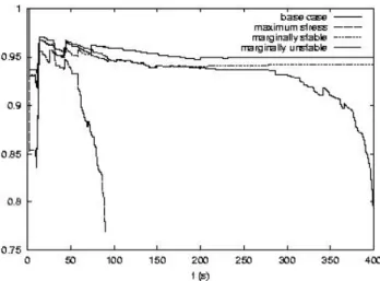
Extensive tests have shown that this power inflow in the Montréal area, with a correction depending on the relative loading of the two transmission corridors, is the most significant power transfer to monitor [11]. Operators are in charge of switching shunt compensation to maintain the 735-kV buses close to their nominal voltage, whathever the power flows. This action is simply accounted for in the pre-contingency load flow by connecting to the buses of concern fictitious synchronous condensers which maintain 1 pu voltages. These are converted to shunt susceptances at the beginning of each QSS simulation. The QSS simulation model includes around 550 buses, 100 generators and 230 LTCs. The time step is 1 s. Figure 4 shows the QSS time evolution of the voltage near Québec City after the most severe contingency (applied at t= 1 s), at four levels of pre-contingency stress S : 0, 0.17 Smax, 0.19 Smaxand Smax. This figure confirms that voltage dynamics are strongly influenced by the MAIS (responsible for the many jumps). The number and timing of reactor trippings strongly influences voltage stability. A static tool like the post-contingency load flow does not allow to guess how many and when switchings take place. Hence, in this system, it was found impossible to pre-filter the contingencies with a load flow. One has to rely on the SBS to filter out contingencies.

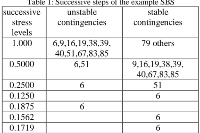
Figure 4: QSS evolutions of a 735-kV bus voltage (in pu) Table 1 describes the various steps of the SBS. The overall SOL is the one of contingency Nb. 6, and is in the interval [0.1719 0.1875] Smax = [516 563] MW. After extensive tests, the parameters of the self-stopping strategy have been set to τ= 65 s, G = -30 MW and G' = 0. These values provide the best saving in computing time without affecting the limits. Figure 5 shows the unrestored load power C(t) for the same contingency but two pre-contingency stress levels. In the stable case, the simulation is stopped at

Table 1: Successive steps of the example SBS successive stress levels unstable contingencies stable contingencies 1.000 6,9,16,19,38,39, 40,51,67,83,85 79 others 0.5000 6,51 9,16,19,38,39, 40,67,83,85 0.2500 6 51 0.1250 6 0.1875 6 0.1562 6 0.1719 6

t= 160 s, when C(t) reaches G'=0. Without this stopping criterion, the simulation would continue up to the maximum of 600 s. Since the system has reached steady state, the computational saving is basically the checking of all discrete devices in between 160 and 600 s. In the unstable case, the simulation is stopped at t= 125 s, i.e. 65 s after C(t) goes through the global maximum at t= 60 s. Without this early stop, the simulation would continue up to 150 s, where some transmission voltages reach 0.8 pu (this is a "no return" point for the system). The figure also illustrates that a too smallτ may lead to identify local maxima.

Figure 5: C(t) in a stable and an unstable case (in MW) In the SBS of Table 1, 92 QSS simulations have been stopped because C(t) reached G' and 13 because a maximum of C(t) was detected.

3.3. Computational efficiency

In order to assess the efficiency and reliability of the filtering procedure, the above set of 90 contingencies has been analyzed in 10 system configurations differing by the lines out of service and/or the number of MAIS. The average computing time on a 500-MHz 128-Mb Pentium III PC (running Windows NT4.0) ranges between 1 min 20 s and 4 minutes. The method is thus fully compatible with real-time requirements. On the average, with respect to the computation of all

individual SOLs, SBS allows to save 50 % of the computing time while SBS together with the self-stopping criterion allows to a 75 % saving.

4. EXAMPLE FROM THE EDF SYSTEM

With a peak load of about 75,000 MW, EDF operates a large system from 7 regional and one national control centers. This system is rather dense and meshed. Much attention is paid to voltage security, especially in the Western and South-East regions where load centers are faraway from generation. However, due to the overall meshed structure, voltage instability modes may be spatially very different from one contingency to another [7].

The example considered hereafter is typical of the VSA to be performed at the national dispatching. The stress is a national load increase (Smax=7000 MW), compensated by French generators. In this context, an explicit modelling of the HV sub-transmission systems cannot be envisaged, due to the huge number of equipments and the lack of real-time data. Instead, the combined response of HV lines, HV-MV transformers and MV-connected loads is represented by an exponential load model, placed behind the EHV-HV transformers, all equipped with LTCs. However, since the HV-MV transformers are also equipped with LTCs, a second, ideal transformer having the typical HV-MV tapping delays and deadband, is placed in between the EHV-HV one and the load, as shown in Fig. 6.

Figure 6: Equivalent load modelling

This transformer has a large number of tapping steps so that it does not hit its limit. Consequently, in a stable scenario, all MV voltages are restored to their setpoints (except for the deadbands) and hence all load powers to their pre-contingency values. This somewhat conservative choice is expected to make SOLs (which correspond to marginally stable cases) less sensitive to load model uncertainties. Compensation shunt capacitors are placed at the HV and MV buses.

In the pre-contingency load flow, loads are increased at the EHV level, while at the beginning of the QSS simulation, each EHV load is replaced by the cascade shown in Fig. 6.

The QSS simulation model includes 1203 EHV and HV bus (real; 90, 63 kV)

MV bus (equivalent) real

ideal equivalent load with

exponential model

512 HV buses, 1024 LTCs4, 176 generator OELs and 15 secondary voltage controllers in the Western and South-East regions. Each of them controls the voltage of some generators so as to keep the voltage of a pilot bus almost constant and the reactive power production of each generator proportional to its capability [12]. A steady-state representation of this control is incorporated to the pre-contingency load flow.

4.1. An example of SOL determination

We consider a set of 105 contingencies involving the two above mentioned regions and including : single and double line outages, single and double generator outages, busbar faults with two to four lines lost. Figure 7 shows the QSS time evolution of the voltage at a Western pilot bus after a severe busbar fault, at four levels of pre-contingency stress S : 0, 0.08 Smax, 0.10 Smax and Smax. The time step is 10 s. The contingency is applied at t= 10 s. The pre-contingency voltage is the same in the first three cases due to secondary voltage control, while at maximum stress the reactive reserves where exhausted. In the base and marginally stable cases, the voltage recovers to almost its pre-disturbance value (although slowly in the latter case).

Figure 7: QSS evolutions of a pilot bus voltage (in pu) In this system with rather smooth post-contingency controls, contingencies can be pre-filtered very efficiently by a post-contingency load, as confirmed by the following results.

A post-contingency load flow is run for each contingency, at maximum stress, and only those contingencies declared potentially harmful will be processed in the SBS. The short-cuts listed at the end of Section 2.6 have been used. In particular :

- load flow is run on the EHV system (the cascades of Fig. 6 are not included);

- secondary voltage control is ignored;

4

the tapping of both EHV-HV and HV-MV transformers is simulated. The HV-MV transformers being ideal, MV buses are not created explicitly, which saves computing time

- load flow divergence is declared as soon as the functionϕ increases or a number of iterations (15) is reached. The latter case corresponds to generators which oscillate between voltage control and reactive power limit, due to a phenomenon analyzed in [13, 2].

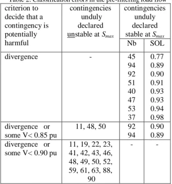
Table 2 lists both the false alarms and the masked contingencies obtained with three filtering criteria. The second choice in the table leads to a good compromize between the two types of errors; the two masked contingencies have a rather high limit. By choosing Smaxlarge enough, the possible pre-filtering errors will not affect the most critical limits.

Table 2: Classification errors in the pre-filtering load flow contingencies unduly declared stable at Smax criterion to decide that a contingency is potentially harmful contingencies unduly declared unstable at Smax Nb SOL divergence - 45 94 92 51 40 47 53 37 0.77 0.89 0.90 0.91 0.93 0.93 0.94 0.98 divergence or some V< 0.85 pu 11, 48, 50 92 94 0.90 0.89 divergence or some V< 0.90 pu 11, 19, 22, 23, 41, 42, 43, 46, 48, 49, 50, 52, 59, 61, 63, 88, 90 -

-The parameters of the self-stopping strategy have been set toτ= 110 s, G = -5 MW and G' = 0, respectively. Figure 8 shows C(t) for the same contingency but two pre-contingency stress levels. In the unstable case, the simulation is stopped at t= 270 s. In the stable case, it is stopped at t= 250 s, when C(t) reaches G'=0.

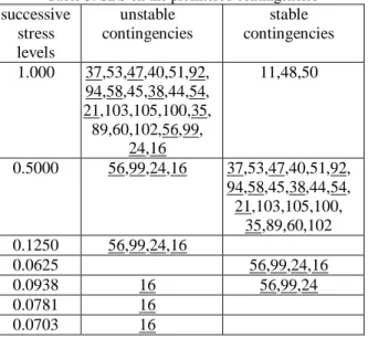
Note that C(t) leaves the zero value in between t= 510 and t= 780 s, due to a voltage oscillation caused by secondary voltage control. Nevertheless, this does not cause instability and it is acceptable to stop the simulation when C(t) reaches zero for the first time. Table 3 describes the various steps of the SBS applied to the 27 contingencies declared potentially harmful by the pre-filtering load flow. The three false alarms are identified by the QSS simulation at maximum stress. The computing time on a 500-MHz PC is 19 s for the pre-filtering load flow and 2 min 30 s for the SBS.

Table 3: SBS on the prefiltered contingencies successive stress levels unstable contingencies stable contingencies 1.000 37,53,47,40,51,92, 94,58,45,38,44,54, 21,103,105,100,35, 89,60,102,56,99, 24,16 11,48,50 0.5000 56,99,24,16 37,53,47,40,51,92, 94,58,45,38,44,54, 21,103,105,100, 35,89,60,102 0.1250 56,99,24,16 0.0625 56,99,24,16 0.0938 16 56,99,24 0.0781 16 0.0703 16

The 13 contingencies underlined in Table 3 involve the Western region, while the others involve the South-East region. With respect to a national load increase, the latter region is thus more robust (in the tested configuration). In order to refine the SOLs of the 11 South-East contingencies, one can process them in an SBS, over the interval [0.5 0.75] Smax. The corresponding computing time is around 1 minute.

5. ADVANCED VOLTAGE SECURITY

ANALYSIS AND CONTROL

In this section we outline recent extensions of the above described VSA tool, which have been successfully tested on the two systems.

These extensions rely on an analysis of the unstable system response to determine the instability mode and identify appropriate remedial actions. We believe that the possibility of retrieving information from unstable scenarii is a definite advantage of (QSS) time simulation.

Practically, this analysis consists of : (i) computing along the system trajectory sensitivities which, when changing sign through infinity, indicate the crossing of a critical point where the Jacobian of the long-term

dynamics has an (almost) zero eigenvalue; (ii) computing the corresponding left eigenvector [14].

5.1. Minimal load shedding

Load shedding is usually considered a post-disturbance, emergency control [1,2]. It is a cost effective solution to face more severe (and hence less probable) contingencies than those considered in preventive VSA.

Pre-disturbance load shedding can be envisaged in a "study mode" in order to assess the severity of a contingency : where and how much load should be shed now in order this contingency not to cause instability ?

To this purpose, the technique proposed in [15] to determine the minimal post-disturbance load shedding can be straightforwardly adapted to pre-contingency. From the above mentioned eigenvector, one can easily obtain a ranking of load buses according to their effectiveness in load shedding. The minimal load shedding is then obtained through a binary search of the type used for determining SOLs. At a given step of this search, shedding is distributed over the load buses in the order given by the above ranking and taking into account the interruptible part of each load.

5.2. Generation rescheduling

Shifting active power generation (closer to critical load centers) can prove useful to increase the insufficient (in particular, negative) security margins of some contingencies.

Let Si* be the system stress at the SOL if the i-th contingency to be corrected (i=1,...,k). Let Sd be the minimum desired value of this stress. Generation rescheduling can be stated as the problem of modifying the generator active powers Pj (j=1,...,n) in an optimal manner so that the k contingencies have their new margin at least equal to Sd. A linearization gives :

Σj Sij (Pj – Pj0) ≥ Sd - Si*(i=1,...,k) (6) where Sijis the sensitivity of Si* to Pj and Pj0 is the base case production of the j-th generator. The sensitivities Sij can be computed from the above mentioned eigenvector [16]. Note that the latter are determined in the post-disturbance configuration, but we assume that they are valid for the pre-contingency situation as well.

The inequalities (6) can be incorporated to an optimal power flow. The simplest form of this optimization problem is the minimum rescheduling problem :

min Σj | Pj – Pj0|

subject to : Σj Sij (Pj – Pj0) ≥ Sd - Si* (i=1,...,k) Pjmin≤ Pj≤ Pjmax (j=1,...,n)

After rescheduling, one contingency should have its margin equal to Sdand the k-1 others should be larger. We found that the linearization is not always accurate enough to meet this objective in a single step, although the relative values of the sensitivities are correct. On the contrary, we found that a second correction (after updating the SOLs) can compensate for this, even without updating the sensitivities.

5.3. Minimal load power margin

When a contingency endangers voltage stability in a limited part only of a large system, it may not be appropriate to measure voltage security through a global load increase. Another viewpoint is to determine the smallest load power margin such that the given contingency would make the system unstable. We consider an L1-norm objective in which the total increase in load power is minimized. Furthermore, to avoid unrealistic loading patterns, we limit each load increase to a specified percentage of the base case power. This problem is "symmetric" to the one of minimal load shedding.

The practical solution consists in modifying the direction of stress during the binary search of the SOL. At a given step of this search, the total loading is distributed over buses in the order given by an eigenvector-based ranking and taking into account the maximum increase specified for each load. By so doing, some loads are increased up to the specified maximum, while others are not increased at all. Hence, the output of this computation is not only a power margin but also the area where loads are increased. In some systems, the ranking can be even based on a snapshot of the unstable voltage profile. The computing time is then merely the one of a conventional binary search.

Contingency filtering at maximum stress is still possible.

BIBLIOGRAPHY

[1] C.W. Taylor, "Power System Voltage Stability", EPRI Power System Engineering Series, McGraw Hill, 1994

[2] T. Van Cutsem and C. Vournas, "Voltage Stability of Electric Power Systems", Power Electronics and Power Systems Series, Kluwer Academic Publishers, 1998

[3] B. Gao, G.K. Morison, P. Kundur, "Towards the development of a systematic approach for voltage stability assesment of large-scale power systems'',

IEEE Trans. on Power Systems, Vol. 11, 1996, No 3, pp. 1314-1324

[4] T. Van Cutsem, C. Moisse, R. Mailhot, "Determination of secure operating limits wih respect to voltage collapse", IEEE Trans. on Power Systems, vol. 14, 1999, pp. 327-335

[5] T. Van Cutsem, Y. Jacquemart, J.-N. Marquet, P. Pruvot, "A Comprehensive Analysis of Mid-term Voltage Stability'', IEEE Trans. on Power Systems, Vol. 10, 1995, pp. 1173-1182

[6] T. Van Cutsem, R. Mailhot, "Validation of a fast voltage stability analysis method on the Hydro-Québec system'', IEEE Trans. on Power Systems, vol. 12, 1997, pp. 282-292

[7] V. Sermanson, C. Moisse, T. Van Cutsem, Y. Jacquemart, "Voltage security assessment of systems with multiple instability modes", Proc. 4th Bulk Power Systems Dynamics and Control (Restructuring) workshop (L. Fink and C. Vournas ed.), Santorini (Greece), Aug. 1998

[8] G.C. Ejebe, G.D. Irisarri, S. Mokhtari, O. Obadina, P. Ristanovic, J.Tong, "Methods for contingency screening and ranking for voltage stability analysis of power systems,'' Proc. PICA conference, 1995, pp. 249-255

[9] E. Vaahedi, C. Fuchs, W. Xu, Y. Mansour, H. Hamadanizadeh, G.K. Morison, "Voltage stability contingency screening and ranking", IEEE Trans. on Power Systems, vol. 14, 1999, pp. 256-265

[10] S. Bernard, G. Trudel, G. Scott, "A 735-kV shunt reactors automatic switching system for Hydro-Québec network'', IEEE Trans. on Power Systems, vol. 11, 1996, pp. 2024-2030

[11] D. Lefebvre, C. Thomassin, "Transits maximums pour la stabilité long terme : limite sud", Hydro-Québec, Div. TransEnergie, Capacité et Stratégie du réseau principal, Internal report, Aug. 1998 (in French) [12] H. Vu, P. Pruvot, C. Launay, Y. Harmand, "An improved secondary voltage control on large-scale power systems'', IEEE Trans. on Power Systems, Vol. 11, 1996, pp. 1295-1303

[13] I. Dobson and L. Lu, "Immediate change in stability and voltage collapse when generator reactive power limits are encountered", Proc. 2nd Bulk Power System Voltage Phenomena (Voltage Stability and Security) workshop (L. Fink editor), Deep Creek Lake (USA), 1991, pp. 65-73

[14] P. Rousseaux, T. Van Cutsem, ``Fast small-disturbance analysis of long-term voltage stability'', Proc. 12th PSCC, Dresden, 1996, pp. 295-302

[15] C. Moors, T. Van Cutsem, "Determination of optimal load shedding against voltage instability'', Proc. 13th PSCC, Trondheim, (Norway), 1999

[16] S. Greene, I. Dobson, F.L. Alvarado, "Sensitivity of the loading margin to voltage collapse with respect to arbitrary parameters'', IEEE Trans. on Power Systems, vol. 12, 1997, pp. 262-272