HAL Id: hal-01254108
https://hal.archives-ouvertes.fr/hal-01254108v2
Submitted on 20 Jan 2016
HAL is a multi-disciplinary open access
archive for the deposit and dissemination of
sci-entific research documents, whether they are
pub-lished or not. The documents may come from
teaching and research institutions in France or
abroad, or from public or private research centers.
L’archive ouverte pluridisciplinaire HAL, est
destinée au dépôt et à la diffusion de documents
scientifiques de niveau recherche, publiés ou non,
émanant des établissements d’enseignement et de
recherche français ou étrangers, des laboratoires
publics ou privés.
Are There Approximate Fast Fourier Transforms On
Graphs?
Luc Le Magoarou, Rémi Gribonval
To cite this version:
Luc Le Magoarou, Rémi Gribonval. Are There Approximate Fast Fourier Transforms On Graphs? .
International Conference on Acoustics, Speech and Signal Processing (ICASSP), Mar 2016, Shanghai,
China. �hal-01254108v2�
ARE THERE APPROXIMATE FAST FOURIER TRANSFORMS ON GRAPHS?
Luc Le Magoarou, R´emi Gribonval
Inria
Centre Inria Rennes - Bretagne Atlantique
ABSTRACT
Signal processing on graphs is a recent research domain that seeks to extend classical signal processing tools such as the Fourier trans-form to irregular domains given by a graph. In such a graph setting, a way to rapidly apply the Fourier transform, i.e. a Fast Fourier Trans-form (FFT), is lacking. In this paper, we propose to leverage the re-cently introduced Flexible Approximate MUlti-layer Sparse Trans-forms (FAµST) in order to compute approximate FFTs on graphs. The approach is first described, then validated on several types of classical graphs and finally used for fast filtering, showing good po-tential.
Index Terms— Graphs signal processing, Fast Fourier Trans-form, matrix factorization.
1. INTRODUCTION
Graphs are ubiquitous in modern data processing. They are indeed a very convenient mathematical tool to represent complex relation-ships that arise naturally when dealing with networked data acqui-sition settings. Recently, methodological tools have been developed that generalize classical signal processing techniques to graph sig-nals, i.e. signals that live on the vertices of a graph instead of a regular grid, as classically assumed in signal processing. Extensive surveys on this topic can be found in [1] and [2]. In particular, the Fourier transform of graph signals can be defined, but no fast algo-rithm has been discovered yet to apply it for general graphs.
In the following, we consider a graph G = (V, E, W), where V and E represent the vertex and edge sets of the graph, and W ∈ Rn×n represents the matrix of edge weights (wijbeing the weight
of an edge connecting vertices i and j), with n = |V| denoting the number of vertices. We assume the graph is connected. We denote by L ∈ Rn×n the combinatorial graph Laplacian matrix, and by
U ∈ Rn×nits eigenvector matrix, with associated eigenvalues in the diagonal matrix Σ ∈ Rn×n.
A Fourier transform on a graph can be defined as the change of basis from the trivial node basis to the basis defined by the eigenvec-tors of L, namely the columns of U (see [1] for a more precise def-inition). Considering a signal x ∈ Rnon the graph, and its Fourier transform y ∈ Rnwe have:
y = UTx x = Uy.
The matrix U being dense in general, the change of basis costs O(n2
) arithmetic operations in both ways, if done using this ba-sic matrix multiplication. However in the case of a regular domain (which can be viewed as a ring graph), it is possible to do the change of basis in O(n log n) arithmetic operations, using the Fast Fourier
This work was supported in part by the European Research Council, PLEASE project (ERC-StG- 2011-277906).
Transform (FFT) [3], which is a linear algorithm (i.e. only made of scalar multiplications and additions) exploiting the factorizability of U into sparse factors1
, U = J Y j=1 Sj. (1)
This factorizability is a necessary and sufficient condition for a fast linear algorithm to exist [4]. In the case of the classical Fourier trans-form, U can be factorized into J = log2(n) factors, each having 2n
nonzero entries. Unfortunately, it is as of today unclear if such a fac-torization can be generalized to more complicated graphs structures. Relaxing the exact factorization constraint, and considering an ap-proximate form of (1), one can wonder: Are there apap-proximate Fast Fourier Transforms on graphs?
We recently proposed the Flexible Approximate MUlti-layer Sparse Transforms (FAµST) [5], an empirical approach to approxi-mate matrices by such multi-layer sparse products. It allows to get computationally efficient approximations for matrices of interest. The approach is based on non-convex optimization techniques and amounts to a hierarchical factorization of the matrix to approximate. It has been applied to dictionary learning [6] and inverse problems [7], showing a good trade-off between accuracy and computational complexity.
Such an approach can be applied to the Fourier matrix U of a graph, in order to try and give an answer to the question asked in this paper. This could be of direct practical interest in applications where the same Fourier matrix has to be applied to a great num-ber of signals. This situation occurs for example when time-varying signals defined on a static graph have to be manipulated in the fre-quency domain (see [8, section VI.A] for an example application of this type).
Objective and contributions. Here, our goal is to show that U can be approximated by a FAµST for a wide variety of graphs, thus defining an approximate FFT for the considered graph. This is done by modifying the previously proposed multi-layer sparse factoriza-tion approach [5] to handle the fact that the FAµST has to diagonal-ize approximately the Laplacian matrix L. We propose in this paper an approach that allows to get FAµSTs with computational complex-ities O(nα), 1 < α < 2, approximating well the true Fourier trans-form of many classical families of graphs as shown in sections 3.1 and 3.2. Moreover, it shows potential for concrete applications such as fast approximate filtering, as attested in section 3.3.
2. OPTIMIZATION FRAMEWORK 2.1. Algorithm
Our goal is to compute a FAµST ˆU =QJ
j=1Sjthat approximates
well the graph Fourier matrix U. One possibility to do so is to di-rectly factorize U into sparse factors, as is done in [7, Algorithm 1]
1The product being taken from right to left:QN
in the case of inverse problems. We refer to this approach as FAµST factorization of the Fourier matrixU in the remaining of the pa-per. However, such a direct factorization does not take into account the fact that the approximate Fourier matrix ˆU has to diagonalize approximately the Laplacian L. We propose next a FAµST diago-nalization of the Laplacian matrixL. The optimization problem at hand is the following:
minimize S1,...,SJ,D 1 4 L − SJ. . . S1DST1 . . . STJ 2 F subject to Sj∈ Sj, ∀j ∈ {1, . . . , J } D ∈ D, (2) where the Sjs are sets of sparse matrices and D is a set of
diago-nal matrices. This problem actually amounts to try and diagodiago-nalize the Laplacian matrix L by a FAµSTQJ
j=1Sj. It is a non-convex
and non-smooth problem, that can be tackled using a Proximal Al-ternating Linearized Minimization (PALM) [9] algorithm, with con-vergence guarantees to a stationary point. Such an algorithm up-dates alternatively each factor by a projected gradient descent step. However, the high number of local minima renders the problem very dependent to initialization.
As first introduced in our previous work [6] for a related prob-lem, instead of directly tackling the problem (2), we propose to re-sort to a strategy in which the true Fourier matrix U is factorized hierarchically. The strategy is to start from the true Fourier matrix U , T0, and factorize it in two factors: U ≈ T1S1, where T1is
called the residual and S1is sparse. The residual is then iteratively
factorized: Ti−1 ≈ TiSi, where kTik0+ kSik0 < kTi−1k0 in
order to make complexity savings at each step (kAk0being a short-hand for kvec(A)k0). A global optimization step is inserted be-tween each 2-factorization in order to stay close to diagonalizing the Laplacian matrix L. This global optimization handles the following subproblem (for increasing values of i):
minimize S1,...,Si,Ti,D 1 4 L − TiSi. . . S1DST1 . . . STiTTi 2 F subject to Sj∈ Sj, ∀j ∈ {1, . . . , i} Ti∈ Ti, D ∈ D, (3) with Tia set of sparse matrices (sparser as i grows). The structure of
the algorithm is given in Algorithm 1. The main steps of this algo-rithm (lines 3 and 4) use PALM, which amounts to alternate updates of the factors by projected gradient steps. Expressions of the projec-tion operators associated to sets of sparse matrices are given in [5], as well as expressions of the gradients implicit in line 3. Expressions of the gradient implicit in line 4 are not given here for brevity reasons, but easily calculated with basic algebra.For a broader exposition of PALM and its application to FAµST, see [5].
Algorithm 1 FAµST diagonalization of the Laplacian matrix Input: Fourier matrix U; Laplacian L; eigenvalues Σ; desired
number of factors J ; constraint sets Siand ˜Si, i ∈ {1 . . . J −1}.
1: T0← U, D ← Σ
2: for i = 1 to J − 1 do
3: Factorization of the residual in 2 factors using PALM [9]: Ti−1≈ TiSi
4: Global optimization with PALM to handle (3): L ≈ TiSi. . . S1DST1 . . . S T iT T i 5: end for 6: SJ ← TJ −1
Output: The estimated factorization: {Sj}Jj=1,D.
2.2. Factorization setting
The usual Fourier transform on a 1D regular grid (corresponding to a ring graph) can be applied in O(n log n) arithmetic operations although the Fourier matrix contains n2 non-zero entries. This is
because the Fourier matrix U can be factorized into log2n factors,
each having 2n non-zero entries. In other words, in the 1D regu-lar grid case we have U = Qlog2n
j=1 Sj, with kSjk0 = 2n. This
factorization corresponds to the usual FFT [3]. In the context of a hierarchical factorization of the Fourier matrix with exponentially decreasing sparsity of the residual (as explained in [5]), we can hope to retrieve this factorization by setting the sparsity of the right factor to 2n and the sparsity of the residual ton2
2i at the ith 2-factorization.
This amounts to dividing the residual sparsity by two at each step, i.,e, a rate of decrease of 2. Such a hierarchical strategy would lead to the sparsity configuration depicted on Figure 1.
Fig. 1. Ideal factorization configuration in the 1D regular grid case. The sparsity of each factor is shown.
Here, our objective is to generalize the multi-layer sparse fac-torization of the Fourier matrix to domains given by an underlying graph, in order to find approximate FFTs for graph signals. Since in that case we do not know if a factorization of the Fourier matrix is possible with factors as sparse as in the 1D regular grid case, we pro-pose to relax the sparsity assumptions in the three following ways: • The number of factors J is reduced by a constant C1 (J =
log2n − C1). This leads to a higher accuracy in the
factoriza-tion (more factors leading empirically to higher error [5]), and allows to reduce the factorization time which is proportional to the number of factors considering the hierarchical strategy of Algorithm 1.
• The rate of decrease of the residual sparsity is reduced to C2with
1 < C2≤ 2. This amounts to dividing the sparsity of the residual
by a number smaller than two at each step of Algorithm 1, leading to a better accuracy of factorization.
• The sparsity of each factor is further multiplied by a constant C3
with C3 > 1. Allowing more non-zero entries in the FAµST this
way logically leads to higher accuracy.
The resulting relaxed factorization configuration is summarized in Figure 2. Such a factorization contains C3.(2n(log2n − C1) +
n2.C1+C1−log2n
2 ) non-zero entries, which is O(n
2−log2C2) for
1 < C2< 2 and O(n log2n) for C2 = 2.
3. EXPERIMENTS
In this section we assess experimentally the performance of the pro-posed method. We first try and give an answer to the main question of this paper, and show that we can get FAµSTs with complexity O(nα
) and good accuracy for various graphs. We then compare the proposed FAµST diagonalization of the Laplacian matrix L to the FAµST factorization of the Fourier matrix U on random sensor graphs. We finally use the approach in a fast filtering scenario on the Minnesota road graph, showing its applicability.
3.1. Approximate FFT for classical graphs
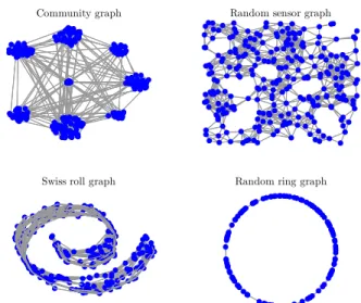
We perform here an experiment in order to show that it is possible to define approximate FFTs on a variety of standard families of graphs. The factorizations are done with different graphs of different sizes, in order to show that the O(nα) settings that were introduced in sec-tion 2.2 are indeed appropriate. We consider five classical random graphs, generated with help of the Graph Signal Processing (GSP) toolbox [10], and taken with their default parameterization (a de-tailed description can be found in [10]). Are considered:
• Erd˝os-R´enyi: a random graph with connection probability p = 0.1.
• Community: a random community graph made of√n/2 com-munities of random sizes.
• Random sensor: a random graph where nodes represent sensors that are placed randomly on the plane.
• Swiss roll: a graph where nodes are placed randomly on the Swiss roll manifold.
• Random ring: a ring graph with random distances between nodes.
Examples of considered graphs are shown in Figure 3.
The experiment amounts to applying Algorithm 1 on these graphs with a fixed setting: C1 = 3, C2 = 1.67 (α = 1.26) and
C3= 1.4 , with a varying number of nodes n ∈ {64, 128, 256, 512}.
The results in terms of relative error with respect to the factorized Laplacian are shown on Figure 4. It can be seen on this figure that for all considered kinds of graphs, the achieved error does not sig-nificantly depend on the graph dimension. The Relative Complex-ity (RC= PJ
j=1kSjk0/n
2
) of the computed FAµSTs decreases when the dimension increases, it follows indeed a O(n−0.74) be-haviour for C2 = 1.67. More specifically with our setting we have
RC= 0.59 for n = 64, RC= 0.37 for n = 128, RC= 0.23 for n = 256 and RC= 0.14 for n = 512. This means that we can factorize the Fourier matrices corresponding to various graphs, with FAµSTs having O(nα) complexities with α < 2. In other words,
the greater the dimension, the higher the complexity savings for the same error, and approximate FFTs can be defined for these graphs.
However, we can see differences in approximation quality be-tween the considered graphs. Indeed , the relative error with respect to the Laplacian is about 10−5for the Swiss roll and the random ring graph, and about 10−1for the Erd˝os-R´enyi graph. Such differences may indicate properties of graphs favorable to Fast Fourier Trans-forms. It seems indeed that graphs with more structure (typically the random ring, related to non-uniform FFT [11]) have Fourier matri-ces that can be better approximated by FAµSTs than unstructured graphs (typically Erd˝os-R´enyi).
3.2. FAµST factorization of U vs FAµST diagonalization of L The objective of this subsection is to compare Algorithm 1 with a FAµST factorization of the Fourier matrix U. For this experiment,
Community graph Random sensor graph
Swiss roll graph Random ring graph
Fig. 3. Example of different graphs with n = 256 nodes (except the random ring that has n = 128 nodes).
64 128 256 512 10−6 10−5 10−4 10−3 10−2 10−1 100 . . L − ˆ U ˆ D ˆ U T . . 2 /F . . L . . 2 F Number of vertices Erd˝os-R´enyi Community Random sensor Swiss roll Random ring
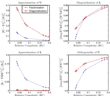
Fig. 4. Factorization error for graphs of different dimensions n ∈ {64, 128, 256, 512}. The mean over 10 independent trials is shown. a random sensor graph with n = 1024 nodes is used. The Fourier matrix U is approximated using either Algorithm 1 (denoted diag-onalizationmethod in the sequel) or the factorization method that is described in details in [5] (denoted factorization method in the sequel). The parameters for both methods are set as follows: • C1 = 3
• C2 ∈ {1.43, 1.67, 2} (it corresponds to FAµSTs of complexity
{O(n1.48), O(n1.26), O(n log
2n)})
• C3 ∈ {1.3, 1.4, 1.5}.
We use the following performance measures:
• Approximation of U: we evaluate the closeness between the original Fourier matrix U and its FAµST approximation ˆU with the quantity ˆU − U 2 F/ U 2
F (this quantity is proportional to
the cost function of the factorization).
• Diagonalization of L: we evaluate how close to diagonal would the Laplacian L be in the basis defined by the columns of ˆU if ˆU was orthogonal, by the quantity
diag( ˆUTL ˆU) 2 F/ ˆUTL ˆU 2 F.
• Approximation of L: we evaluate the closeness between the graph Laplacian L and its approximation by the quantity L −
ˆ U ˆD ˆUT 2 F/ L 2
F(we consider that ˆD = Σ in the factorization
case, and this quantity is proportional to the cost function of the diagonalization).
• Orthogonality of ˆU: we evaluate how close to orthogonal ˆU is with the quantity diag( ˆU ˆUT)
2 F/ ˆU ˆUT 2 F.
The results of these approximations are given in Figure 5. Several comments are in order. First of all, as expected, the approximation
of U is better in the factorization case, compared to the diagonaliza-tion case, since it is the objective of the factorizadiagonaliza-tion. Similarly, the approximation of L is better in the diagonalization case. Second, the diagonalization of L is performed similarly by the two methods, ex-cept for low relative complexities where the diagonalization method seems better. Third, ˆU is closer to orthogonal using the diagonal-ization method, for any relative complexity. In conclusion, the di-agonalization method yields approximate fast Fourier transforms ˆU that exhibit better properties in terms of orthogonality, approxima-tion of the Laplacian and diagonalizaapproxima-tion of the Laplacian. On the other hand, they approximate the original Fourier matrix U less well than the FAµSTs computed using the factorization method, but this criterion seems less relevant than the others that measure properties that are intrinsically expected of the graph Fourier transform.
0 0.05 0.1 0.15 0.2 0 0.1 0.2 0.3 0.4 0.5 0.6 0.7 Approximation of U .. ˆ U− U .. 2/F .. U .. 2 F Relative Complexity (RC) Factorization Diagonalization 0 0.05 0.1 0.15 0.2 0.84 0.86 0.88 0.9 0.92 0.94 0.96 0.98 Diagonalization of L .. d ia g ( ˆ U TL ˆ U) .. 2/F .. ˆ U TL ˆ U .. 2 F Relative Complexity (RC) 0 0.05 0.1 0.15 0.2 0 0.05 0.1 0.15 0.2 Approximation of L .. L − ˆ U ˆ D ˆ U T .. 2/F .. L .. 2 F Relative Complexity (RC) 0 0.05 0.1 0.15 0.2 0.8 0.85 0.9 0.95 1 Orthogonality of ˆU .. d ia g ( ˆ U ˆ U T) .. 2/F .. ˆ U ˆ U T .. 2 F Relative Complexity (RC)
Fig. 5. Approximation results on the random sensor graph with n = 1024 nodes. The diagonalization and factorization methods are compared.
3.3. Fast filtering on the Minnesota road graph
The objective of this subsection is to use the FAµSTs approxi-mations computed by Algorithm 1 and the factorization method of [5] for fast filtering on the Minnesota road graph, in order to show the applicability of our approach. This experiment should be taken as a proof of concept, showing that filtering signals on graphs using a FAµST ˆU instead of the true Fourier matrix U makes sense. Signal model. For this experiment, a low-pass signal x is gener-ated randomly in the graph frequency domain: the components of its spectrum are independent and follow a normal distribution of stan-dard deviation θ = exp(−f ), where f is the frequency (eigenvalues of the Laplacian). This reference signal is then corrupted by a white Gaussian noise nv N (0, σ). This gives a noisy signal ˜x = x + n. Filtering. The corrupted signal is low-pass filtered by a filter of fre-quency response h(f ) = 1/(1 + γf ) with γ = 3. The filtering is done using either the true Fourier transform matrix U, a FAµST
ˆ
Udiagcomputed by diagonalization, or a FAµST ˆUfactcomputed by
factorization. The setting presented in section 2.2 is used in both cases with C1 = 3, C2 = 1.43 and C3 = 1.5. In this
configura-tion, ˆUdiag and ˆUfactexhibit a relative complexity of 0.13 (they are
approximately eight times faster than U).
Results. SNR results are given for different noise levels σ and in av-erage over several realizations in Table 1. Filtering using a FAµST
as an approximate Fast Fourier Transform on graph is shown to be almost as good as classical filtering using the actual Fourier matrix (less than one decibel of difference), although it is more computa-tionally efficient (eight times). Moreover, the factorization technique seems to provide better filtering performance than the diagonaliza-tion. An example of filtering is shown in Figure 6.
σ = 0.3 σ = 0.4 σ = 0.5 σ = 0.6 Noisy 1.82 -0.68 -2.65 -4.25 Filtered with U 5.11 4.57 3.89 3.22 Filtered with ˆUdiag 4.04 3.62 3.11 2.60
Filtered with ˆUfact 4.70 4.23 3.59 2.98
Table 1. Filtering results, the SNRs in decibels and in average over 100 independently drawn signals for each noise level are given.
Clean signal −1.5 −1 −0.5 0 0.5 1 Noisy signal, SNR=-4.30dB −1.5 −1 −0.5 0 0.5 1
Filtered signal using U, SNR=3.40dB
−1.5 −1 −0.5 0 0.5 1
Filtered signal using ˆUf act, SNR=3.08dB
−1.5 −1 −0.5 0 0.5 1
Fig. 6. Example of filtering on the Minnesota road graph. Classical filtering using U and filtering using a FAµST ˆUfactare shown.
4. DISCUSSION AND CONCLUSION
In this paper, we showed that many graphs admit an approx-imate fast Fourier transform, by approxapprox-imately diagonalizing the graph Laplacian L with a FAµST ˆU = QJ
j=1Sj. The approach
was validated on several random graphs, compared to a direct ap-proximate factorization of the Fourier matrix U and tested on a fast graph signal filtering task with promising results.
Such an approach is well suited to situations where the graph is fixed, and the Fourier transform has to be applied rapidly a great number of times. This is to amortize the factorization cost. Such a situation corresponds for example to real-time monitoring of graph signals, where a threshold on the high-frequency components of the signal is set to detect anomalies, as is done in [8, section VI.A].
In future work, and in order to reduce the computation time, one could imagine to directly diagonalize the graph Laplacian without even requiring the true Fourier matrix as input. This would amount initialize T0 and D differently in Algorithm 1. Indeed, the
initial-izations proposed in this paper (T0← U, D ← Σ) require an exact
diagonalization of the graph Laplacian prior to the hierarchical fac-torization. Another interesting perspective would be to take advan-tage of the versatility of the used optimization algorithm to enforce some properties on the factorization. For example, if the targeted application is filtering, one could imagine enforcing a better recon-struction of eigenvectors corresponding to small eigenvalues, used for low-pass filtering.
5. REFERENCES
[1] David I Shuman, Sunil K Narang, Pascal Frossard, Antonio Or-tega, and Pierre Vandergheynst, “The emerging field of signal processing on graphs: Extending high-dimensional data analy-sis to networks and other irregular domains,” Signal Processing Magazine, IEEE, vol. 30, no. 3, pp. 83–98, 2013.
[2] Aliaksei Sandryhaila and Jose M.F. Moura, “Big data analy-sis with signal processing on graphs: Representation and pro-cessing of massive data sets with irregular structure,” Signal Processing Magazine, IEEE, vol. 31, no. 5, pp. 80–90, Sept 2014.
[3] James Cooley and John Tukey, “An algorithm for the machine calculation of complex Fourier series,” Mathematics of Com-putation, vol. 19, no. 90, pp. 297–301, 1965.
[4] Jacques Morgenstern, “The linear complexity of computation,” J. ACM, vol. 22, no. 2, pp. 184–194, Apr. 1975.
[5] Luc Le Magoarou and R´emi Gribonval, “Flexible multi-layer sparse approximations of matrices and applications,” CoRR, vol. abs/1506.07300, 2015.
[6] Luc Le Magoarou and R´emi Gribonval, “Chasing butterflies: In search of efficient dictionaries,” in Acoustics, Speech and Signal Processing (ICASSP), 2015 IEEE International Confer-ence on, April 2015.
[7] Luc Le Magoarou, R´emi Gribonval, and Alexandre Gramfort, “FAµST: speeding up linear transforms for tractable inverse problems,” in EUSIPCO , Nice, France, Aug. 2015.
[8] Aliaksei Sandryhaila and Jose M.F. Moura, “Discrete signal processing on graphs: Frequency analysis,” Signal Processing, IEEE Transactions on, vol. 62, no. 12, pp. 3042–3054, 2014. [9] J´erˆome Bolte, Shoham Sabach, and Marc Teboulle, “Proximal
alternating linearized minimization for nonconvex and nons-mooth problems,” Mathematical Programming, vol. 146, no. 1-2, pp. 459–494, 2014.
[10] Nathana¨el Perraudin, Johan Paratte, David Shuman, Vassilis Kalofolias, Pierre Vandergheynst, and David K. Hammond, “GSPBOX: A toolbox for signal processing on graphs,” ArXiv e-prints, Aug. 2014.
[11] A. Dutt and V. Rokhlin, “Fast fourier transforms for nonequi-spaced data,” SIAM J. Sci. Comput., vol. 14, no. 6, pp. 1368– 1393, Nov. 1993.