HAL Id: hal-02154536
https://hal.archives-ouvertes.fr/hal-02154536
Submitted on 12 Jun 2019
HAL is a multi-disciplinary open access
archive for the deposit and dissemination of sci-entific research documents, whether they are pub-lished or not. The documents may come from teaching and research institutions in France or abroad, or from public or private research centers.
L’archive ouverte pluridisciplinaire HAL, est destinée au dépôt et à la diffusion de documents scientifiques de niveau recherche, publiés ou non, émanant des établissements d’enseignement et de recherche français ou étrangers, des laboratoires publics ou privés.
to scale: a spatial hedonic approach in Brittany
Abdel Fawaz Osseni, François Bareille, Pierre Dupraz
To cite this version:
Abdel Fawaz Osseni, François Bareille, Pierre Dupraz. Decoupling values of agricultural externalities according to scale: a spatial hedonic approach in Brittany. [University works] Inconnu. 2019, 49 p. �hal-02154536�
to scale: a spatial hedonic approach in Brittany
Abdel Fawaz OSSENI, François BAREILLE, Pierre DUPRAZ
Working Paper SMART – LERECO N°19-04
May 2019
UMR INRA-Agrocampus Ouest SMART - LERECO
Les Working Papers SMART-LERECO ont pour vocation de diffuser les recherches conduites au sein des unités SMART et LERECO dans une forme préliminaire permettant la discussion et avant publication définitive. Selon les cas, il s'agit de travaux qui ont été acceptés ou ont déjà fait l'objet d'une présentation lors d'une conférence scientifique nationale ou internationale, qui ont été soumis pour publication dans une revue académique à comité de lecture, ou encore qui constituent un chapitre d'ouvrage académique. Bien que non revus par les pairs, chaque working paper a fait l'objet d'une relecture interne par un des scientifiques de SMART ou du LERECO et par l'un des deux éditeurs de la série. Les Working Papers SMART-LERECO n'engagent cependant que leurs auteurs.
The SMART-LERECO Working Papers are meant to promote discussion by disseminating the research of the SMART and LERECO members in a preliminary form and before their final publication. They may be papers which have been accepted or already presented in a national or international scientific conference, articles which have been submitted to a peer-reviewed academic journal, or chapters of an academic book. While not peer-reviewed, each of them has been read over by one of the scientists of SMART or LERECO and by one of the two editors of the series. However, the views expressed in the SMART-LERECO Working Papers are solely those of their authors.
1
Decoupling values of agricultural externalities according to scale: a spatial
hedonic approach in Brittany
Abdel Fawaz OSSENI
INRA, UMR1302 SMART-LERECO, 35000, Rennes, France
François BAREILLE
INRA, UMR1302 SMART-LERECO, 35000, Rennes, France Université de Bologne, DISTAL, 40127 Bologne, Italie
Pierre DUPRAZ
INRA, UMR1302 SMART-LERECO, 35000, Rennes, France
Acknowledgements
This project is funded by the H2020 European project PROVIDE (http://www.provide-project.eu).
The authors would like to acknowledge the two referees for their valuable comments as well as the
participants to the 35èmes Journées de Microéconomie Appliquée. The authors acknowledge also
Yves Surry and Philippe Le Goffe for their helpful suggestions at the beginning of this project.
Corresponding author:
François Bareille
INRA, SMART-LERECO
4 allée Adolphe Bobierre, CS 61103 35000 Rennes, France
Email : francois.bareille@inra.fr Phone: +33 (0)2 23 48 53 84 Fax: +33 (02) 23 48 53 80
Les Working Papers SMART-LERECO n’engagent que leurs auteurs.
2
Decoupling values of agricultural externalities according to scale: a spatial hedonic approach in Brittany
Abstract
Agricultural activities jointly generate various externalities. Hedonic pricing method allows for their valuation. Previous hedonic studies have estimated the value of the externalities generated by a given agricultural activity in a single parameter. Based on simple theoretical model, we illustrate that this parameter captures the sum of the different externalities generated by the activity. We explain that this parameter can differ at different spatial scale. Using specific spatial econometric models with spatial lags on the explanatory variables, we distinguish between the value of infra-municipal agricultural externalities and the value of extra-municipal agricultural externalities with larger spatial range arising from the same agricultural source. Among the estimated models, the spatial lag of the exogenous variable and the general nested spatial models are selected as the best models. We find that swine activities present negative effects at all scales whereas dairy cattle activities, including grassland management, present negative effects at the infra-municipality scale but positive spillovers.
Keywords: externalities, nitrogen, agriculture, spatial econometric
3
Externalités et distances: une spatialisation de l’approche hédonique en Bretagne
Résumé
Les activités agricoles produisent diverses externalités dont la valeur peut être théoriquement estimée à l’aide de la méthode des prix hédoniques. Les études hédoniques antérieures ont toutefois estimé la valeur des externalités générées par une activité agricole à travers un paramètre unique. Sur la base d’un modèle théorique simple, nous montrons que ce paramètre capture la somme des différentes externalités générées par l’activité. Nous expliquons que ce paramètre peut différer à différentes échelles géographiques. En utilisant des modèles économétriques spatiaux spécifiant un effet spatial spécifique pour chaque variable explicative, nous distinguons la valeur moyenne des externalités agricoles capturée à l’échelle infra-communales (où les résidents et les activités agricoles sont localisés dans la même municipalité) et celle capturée à l’échelle extra-municipale (où les résidents et les activités agricoles sont localisés dans des municipalités différentes). Parmi les modèles estimés, les modèles SLX et GNS apparaissent statistiquement comme les meilleurs modèles. Nous montrons que les activités d’élevages porcins et avicoles affectent négativement les résidents à toutes les échelles, tandis que les activités d’élevages bovins, incluant la gestion des prairies, présentent des effets négatifs à l’échelle infra-municipale, mais des effets positifs à l’échelle extra-municipale.
Mots-clés : externalités, azote, agriculture, économétrie spatiale
4
Decoupling values of agricultural externalities according to scale: a spatial
hedonic approach in Brittany
1. Introduction
Agriculture is a multifunctional activity that ensures the joint production of marketable and non-marketable goods. These externalities impact the population’s utility, either positively (e.g. conservation of biodiversity) or negatively (e.g. odor pollution), and present public good features: non-rivalry between consumers and/or non-excludability, especially for nuisances. The modernization of agriculture in Europe during the 20st century has increased the negative agricultural externalities (e.g. Sutton et al., 2011). The authorities have thus implemented several policies to internalize these effects. For example, the Common Agricultural Policy (CAP) offers payments to maintain specific areas (e.g. permanent grasslands) or to help European farmers to modernize their farms and buildings to reduce pollution. The role of the authorities is to establish the most efficient instruments and to allocate an appropriate agro-environmental budget, which notably depends on the benefits captured by the population. These benefits should be estimated using monetary valuation methods. The hedonic pricing method is a cornerstone of this literature (Rosen, 1974). Based on Lancaster’s theory (1966), the hedonic pricing method is based on the principle that prices of marketable goods are defined by the combination of their attributes, which allows the value of each attribute to be determined. This method has been frequently used to estimate the population’s willingness to pay (WTP) to improve environmental conditions, such as water quality (Leggett and Bockstael, 2000), or to reduce negative externalities, such as noise pollution (Fernández-Avilés et al., 2012). The hedonic pricing method is often applied to real estate observations, the theory being that, ceteris
paribus, houses with superior amenities (negative externalities) have a higher (lower) price
corresponding to the capitalization of the externality in the houses’ value.
Several studies have valued agricultural externalities using this method. Le Goffe (2000) found that to double nitrogen concentration at the municipality scale decreases Breton Bed and Breakfast renting prices by 3%. Ready and Abdalla (2005) found that a new livestock farm located 500 meters from a house decreases its value by 6.4%. Herriges et al. (2005) stated that animal facilities reduce property values by 15% when they are located 0.25 miles upwind from houses. Bontemps et al. (2008) found that nitrogen surplus at the municipality scale decreases Breton house prices up to 7% but has no additional effect after 80 kg/Ha. They also found that
5
the municipal share of temporary grassland decreases house prices up to 3%. Cavailhès et al. (2009) found that farmed activities have higher impacts when they are visible from the house. Even if these papers provide remarkable insights on the impacts of agriculture on residents’ utility, they have estimated the hedonic function at a given spatial scale, either the municipal scale (Bontemps et al., 2008; Le Goffe, 2000) or a lower one (Cavailhès et al., 2009; Ready and Abdalla, 2005). They do not provide information on the impacts of agriculture at higher scales, which is however important when designing agro-environmental policies. Indeed, using declared preference methods, several papers highlights that residents are willing to pay to conserve distant sources of amenities (even located from more than one hour to their house), even if the WTP decreases with the distance to the amenity source (e.g., Ay et al., 2017; Pate and Loomis, 1997). As rural households use to move over larger distance than urban ones to reach a place (for their job or leisure activities), agricultural activities can influence the housing market at larger scales than the previously examined ones, at least in neighboring municipalities. In addition, farms are dispersed over space and operate rarely on a single municipality. For example, Breton swine farmers are willing to apply manure at 70 kilometers from their headquarters (Gaigné et al., 2011), which imply that the externalities should not be contained in the municipality where the swine production occurs.
Previous papers have also ignored that agriculture supports the joint provision of several public goods and bads. For example, agricultural wetlands provide habitat for remarkable biodiversity, which can be valorized by hikers, hunters and anglers, but agricultural wetlands are also located in areas with higher flooding risk. One can thus consider that an agricultural activity is a proxy of several public goods, whom quantities are unobserved in the usual datasets. As papers on the distance-decay of WTP highlight that each public good affects agents under its own spatial range of impacts (e.g. Ay et al., 2017; Rolfe and Windle, 2012), one can even consider than an agricultural activity at a given localization is the proxy of several externalities, each of them impacting differently the residents’ utility over space. The consequence is that one agricultural activity can have a positive impact at a narrow scale and a negative impact at a larger scale, and vice versa.
The objective of our paper is to distinguish the value of the agricultural externalities arising from the same agricultural activity at two different scales: the infra-municipal scale (where the residents and the agricultural activities are localized in the same municipality) and the extra-municipal scale (where the residents and the agricultural activities are localized in different municipalities), the distance to the considered activity being smaller in the infra-municipal
6
scale. Our results could inform policymakers on the strengths and forms of the agricultural externalities over space, which should impact the design of agro-environmental policies. For our purpose, we estimate a spatial hedonic model on the rural housing market of Brittany between 2010 and 2012. Spatial hedonic studies has been developed since the seminal work of Leggett and Bockstael (2000) (see Anselin and Lozano-Gracia, 2009 for a review) but have mainly relied on the spatial autoregressive (SAR) model or the spatial error model (SEM), which capture the whole spatial effect in a single parameter (McMillen, 2012). Here, we use econometric models that specify spatial effects for each of the explanatory variable, which are more flexible in modeling spatial spillover effects, i.e. the impact of a change in the variable level at one localization on the dependent variables of other places (Halleck Vega and Elhorst, 2015). The distinction between direct (i.e. the impact of a change in the variable level at one localization on the dependent variables of this localization) and spillover effects allow disentangling the value of agricultural effects at the different identified scales. We test the statistical performance of eight theoretically consistent spatial hedonic models, with four models that include the spatial effects on the explanatory variables. We find that the best specifications are the ones that include the spatial effects on the explanatory variables and in particular the spatial lag of exogenous variable model (SLX) and the general nested spatial model (GNS). This suggest that the principal source of spatial interactions is due to the spillovers of the agricultural externalities. The introduction of these spatial interactions suites better our data than the specifications of the spatial interactions due to price diffusion (captured by SAR and its developments) or due to spatial heterogeneity (captured by SEM and its developments). In particular, we find that swine and poultry breeding activities impact house prices even in neighboring municipalities, suggesting a larger spatial impact than what had been previously estimated. We find that cattle activities (animal density, areas of temporary and permanent grasslands) have a direct negative impact on house prices but a positive spillover on neighboring house prices.
The next section presents a brief theoretical analysis on the measure of agricultural externalities at different scales and explain in more details the interest of the used spatial econometric models. The third section presents the empirical model and the descriptive statistics of the data. The fourth section presents the results of our estimations and the sensitivity analysis. We discuss the results in the last section.
7
2. Advances in spatial hedonic pricing
This section first explains the signification of the estimated parameters in hedonic method when considering a given agricultural activity as the support of different externalities with specific spatial range of impacts. We then present the developments of spatial econometrics to capture the spillover effects at the extra-municipal scale arising from the explanatory variables.
2.1. Hedonic pricing method in a spatial framework
This part departs from the hedonic pricing model developed by Rosen and add successively the different source of spatial interactions that have been identified in the literature: the price diffusion effect, the spatial heterogeneity effect and the diffusion of externalities. The modeling of the diffusion of externalities in a hedonic model have not been theoretically examined to our knowledge.
2.1.1. Hedonic pricing method: basic features
The hedonic pricing method considers that goods, and in particular houses, are functions of their attributes (Ball, 1973; Rosen, 1974). Denoting yi as a vector of n characteristics
1
(yi,...,yni) of house i (i
1;I ) , which can be considered as marketable attributes, zj as a vector of m characteristics (z1j,...,zmj) of localization j ( j
1;J ), including the agricultural activities at the source of the externalities, and Pij as the price of house i in localization j , the hedonic price function is classically written as follows:( , )
ij i j
P Py z (1)
Assuming that the consumer utility U localized in house ij i in municipality j is a function of the consumer’s composite consumption (
x
), yi and zj, U is defined as follows: ij
, ,
ij i j
U U x y z (2)
Under the assumption that consumers maximize their utility under their income constraint
x ij
R p xP , with R being the income of the consumer and px the price of the composite good x, we reach the following first-order condition:
8 ij kj ij ij kj U z P U x z (3)
The term Pij zkj represents the consumer’s marginal WTP for the attribute zkj (the kth element of zj). In particular, zkj can be an agricultural attribute, whom values follow a continuous distribution (e.g. an area or an animal density). Previous studies have focused on the estimation of Pij zkj, providing information on the household valuation of zkj. Assuming a negligible impact of agricultural contractible labor on residents’ localization choices, it means that zkj support the provision of goods and/or services with public good characteristics.
2.1.2. Hedonic pricing method: the price diffusion effect
Relation (3) is valid under some assumptions, namely that (i) all buyers and sellers on house market have perfect information about the attributes’ levels associated to each property’s location, (ii) all buyers in the market are able to move to utility-maximizing positions, (iii) the housing market is in equilibrium and (iv) that the house supply is fixed in the short term (Hanley et al., 2009). The hedonic valuation literature has paid attention to the first assumption by considering that sellers and buyers obtain information about nearby properties and use it to determine the prices of other houses (e.g. Kim et al., 2003). One way to incorporate this information is to consider that the hedonic function depend on the vector P of house prices in the considered market such that Pij P( ,y z Pi j, ). This reflects that buyers and sellers could use
similar neighboring sales as a reference for determining a transaction price (Osland, 2010). Thus, a marginal change in zkj will indirectly impact Pil (j ≠ l) through price reorganization. Assuming that I is the number of houses in localization l (such that l I
Jl1Il ), the total effect of a marginal change of zkj is:1 1 1 1 1 1 1
total impact direct impact price diffusion of attribute of attribute in location in location
1
j l I l n I I I J J J ij il on ml l i kj i kj l m n o ml ij k k j jP
P
P
P
z
z
P
P
(4)9
Such price diffusion effect in housing prices is sometimes subject to criticism (e.g. Anselin and Lozano-Gracia, 2009) because it implies theoretically that all buyers and sellers take simultaneously into account the prices in other transactions, which is unlikely to arise in real settings. Based on this explanation, Anselin and Lozano-Gracia (2009) suggest that the adjacency effect (i.e., the fact that a house price tends to be similar to the prices of neighboring houses) is not due to information diffusion on prices but rather to spatial heterogeneity or to the diffusion of externalities.
2.1.3. Hedonic pricing method: the spatial heterogeneity effect
As already stated, relation (3) means that zkj support the provision of goods and services with public good characteristics. We note
z(1)kj ,...,zkj( )Q
the set of Q public goods and bads supported by zkj, the elements could being be null for some agricultural activities and non-null for the others. The element ( )qkj
z is thus the level of public good q supported by the activity k in the municipality j. We assume that the production of ( )q
kj
z depends on zkj such that
( ) ( ) , q q kj k kj z f z lj , where ( )q kf is the production function of the public good q supported by the activity k, and lj the vector of local conditions (e.g. wind, soil or slope) that may influence the provision of public goods by the agricultural activity k in location j. These local conditions imply that the provision for any public goods supported by k would be heterogeneous over space.
We assume that each of the Q public goods is valued by the households such that
(1) ( )
, , ,..., Q
ij i j j
U U x y z z , with U
being linear. In this framework, Pij zkj is in fact the sum of the value of all Q externalities supported by the attribute zkj. Indeed, relation (3) gives:
( ) ( ) 1 , Q ij kj ij q k kj q q ij kj U z P f z U x z
lj (5)where f k( )q is the marginal productivity of zkj for the production of the public good q, which
is independent to the distance, and Pij zkj q is the value of the externality q supported by activity zkj on house i. This value can be positive or negative. Relation (4) highlights that the estimated WTP for a specific agricultural activity in previous studies is equal to the sum of the
10
values attributed to the externalities jointly produced by the activity. However, as ( )q kj
z is often
unobserved by the econometrician, the Pij zkj q cannot be measured independently and the econometrician can only measure the WTP for a specific activity zkj.
The econometrician could assume that lj does not influence the public good provision such that he could directly estimate relation (3). In particular, a positive value in relation (3) implies that
kj
z provides more positive externalities than negative ones. Alternatively, the econometrician could recognize that lj does influence the public good provision and thus estimates:
,
ij ij kj ij kj P U z U x z j j z l (6)where Pij
z lj, j
zkjreflects the WTP for the attribute k in j that depends on the local conditions. For example, the value of odor nuisance induced by swine density depends on the wind. As these local conditions tend to be correlated over space (see e.g. wind strength or soil quality), the WTP for the activity k could be heterogeneous over space. The econometrician could control for this heterogeneity, which otherwise would lead to biased estimated WTP. In the case where both the spatial heterogeneity and the price diffusion effect appears in the data, the hedonic specification would capture the total effect of a marginal change of zkj as:
1 1 1 1 1 1 1
total impact direct impact price diffusion of attribute of attribute in location in location
, ,
1
j l I l n I I I J J J ij il on ml l i kj i kj l m n o ml ij k k j jP
P
P
P
z
z
P
P
z l P
j j
(7)2.1.4. Hedonic pricing method: the diffusion of externalities
Finally, some papers on the distance-decay effect on WTP illustrate that each public good q supported by activity zkj can impact the residents’ utility in other locations (i.e.
11 ( ) ( ) ( , , , ) ij i j U U x y zq zlq with ( )q l
z being the matrix of the J 1 vectors of the set of public goods
( )
l
q
z in the other locations than j ).1 The total effect of a marginal change of kj z is:
( ) ( ) ( ) 1 1 1 1direct impact local spillovers total impact of unobserved of uno of attribute externality in location supported by in location , j l I I Q J ij q il il k kj q q l i kj i q kj kj k q j k j P P P f z z z z
lj
( ) 1 1 1 bserved externality supported by in location , l I Q J q k kj l i q l j q k j f z
lj (8) where ( )q il kj P z is the spillover of the externality generated by ( )q kj
z in the localization l. Indeed, due to data limitation on the spatial distribution of the agricultural activities, we can only know the municipal implantation of the different activities but, contrary to houses, we ignore their precise localization in the considered municipality.2 Hence, the modeling framework integrates the insights from the distance-decay effect by considering two discrete zones: the municipality j where the agricultural activity zkj occurs (i.e. the infra-municipal scale) and all the other municipalities (i.e. the extra-municipal scale), the infra-municipal scale being localized closer to the externality sources than extra-municipal scale but representing a smaller area than the extra-municipal scale.3
According to the papers on the distance-decay of WTP, the direct impact of the marginal change of ( )q
kj
z should be stronger than any spillover effect, i.e. ( )q ( )q ij kj il kj
P z P z
. For example, a permanent grassland would impact more the utility of hunters that live in the same location than the utility of the hunters that live in other locations. However, as the number of hunters outside from j is supposed greater than the number of hunters in j , the sum of the spillover effects can be higher than the sum of the direct impact depending on the strength of the
distance-decay effect, i.e. ( ) ( )
1 1 1 j l I q J I q l ij kj il kj i i l j P z P z
. This means that the sum of the utilityof hunters derived from the conservation permanent grasslands at the infra-municipal scale can be lower than the sum of the utilities of the hunters that live in other locations (i.e. at the extra-municipal scale).
1 For sake of simplification, we note
( ), ( )
j q q (q) l z z z and 1 J j zj z.
2 We here assume that the
j
z are localized on the centroid of the municipality.
3 Given our assumptions, one can thus consider that the houses of municipality j are closer to the source of the externalities zj than the houses located in other municipalities. Of course, there are cases where houses located in neighbored municipalities can be closer to at least one house of j but this is true on average.
12
As the public goods and bads are jointly produced by zkj and given their wide range of forms and values over space, we can observe cases where the direct and spillover impacts have the same sign and other where they have opposite ones. This feature is presented in Figure 1. In this theoretical example, the activity z provides one public good 11 (1)
11
z and one public bad (2) 11
z
. Figure 1 highlights that, even if the average effect of z is negative in the first municipality 11
(because the effects of z11(2) on the prices of the first municipality are greater than the effects of
(1) 11
z ), the form of the distance-decay explains that the average spillover effect of z is positive. 11
Taking an illustrative case, permanent grasslands in one localization provide suitable conditions to hunters over a large range of space (corresponding to z11(1)) but also represent an area with higher flooding risks (which corresponds to (2)
11
z ). Flooding risk affects houses on a smaller range of space than the suitable hunting conditions but present a higher marginal value in the short range.
Figure 1: joint production of public goods and the distance-decay effect of consumers’ willingness to pay
13
Even if ( )q kj
z is unobserved, the econometrician can assess Pij zkj and Pil zkj
( l
1;J - j) summing over the Q public goods and bads. In this case, relation (8) leads to:1 1 1 1 1
spillovers total impact direct impact
of attribute of attribute of attribute in location in location in location j l I l I I J J ij il il l i kj i kj l i kj l j k k k j j j P P P z z z
(9)in case where the econometrician assumes that local conditions does not affect the public good provision. Alternatively, if the econometrician considers that the local conditions could affect the public good provision, relation (8) leads to:
1 1 1 1 1
total impact direct impact spillovers of attribute of attribute of attribute in location in location in location
, , j l I l I I J J ij il il l i kj i kj l i kj l j k k k j j j P P P z z z
z lj
z lj (10)Relations (9) and (10) present the hedonic specifications without the price diffusion effect. Assuming that such process are at stake in the observations, the econometrician could measure:
1 1 1 1 1 1 1
total impact direct impact price diffusion of attribute of attribute in location in location 1 j l I l n I I I J J J ij il on ml il l i kj i kj l m n o ml ij k k j j P P P P P z z P P z
1 1 1 1 1 1spillovers price diffusion of attribute in location 1 l l n I I I J J J on ml l i kj l m n o ml ij l j k j P P P P
(11)in case he assumes spatial homogeneity. Alternatively, in case of spatial heterogeneity, the econometrician could measure:
1 1 1 1 1 1 1
total impact direct impact price diffusion of attribute of attribute in location in location , , 1 j l I l n I I I J J J ij il on ml l i kj i kj l m n o ml ij k k j j P P P P z z P P
z l Pj
1 1 1 1 1 1spillovers price diffusion of attribute in location , , 1 l l n I I I J J J il on ml l i kj l m n o ml ij l j k j P P P z P P
z l Pj
(12)The three spatial processes (the price diffusion, the spatial heterogeneity and the diffusion of externalities) are at stake in relation (12). To our knowledge, the measure between direct impacts at the infra-municipal scale and spillover impacts at the extra-municipal scale as presented in equations (9) to (13) has never been done in hedonic valuation of agricultural externalities. This is the aim of this paper.
14
2.2. Advances in spatial econometrics: integrating spillovers
The different hedonic specifications that we developed in 2.1 correspond to different spatial econometric models. Indeed, Elhorst (2014) considered three types of spatial interactions to address the spatial effects: (i) the interactions among dependent variables, (ii) the interactions among explanatory variables and (iii) the interactions among the error terms. In the context of the hedonic valuation, the first type of interactions refers to the price diffusion effect (equation (4)), the second type of interactions refers to the diffusion of the externalities (equation (9)) and the third type of interactions refers to the spatial heterogeneity effect (equation (6)). All these interactions can be present in a given set of observations.
To our knowledge, three studies have used spatial econometrics to assess the value of agricultural externalities: Kim and Goldsmith (2009) used the SAR model (equation (4)), Eyckmans et al. (2013) used the spatial autoregressive model with autoregressive disturbances (SARAR) model (equation (7)) and Yoo and Ready (2016) used the SEM (equation (6)). These models do not considered interactions among explanatory variables, i.e. do not consider the diffusion of externalities. Indeed, if the SEM does not consider any indirect impact, the spillovers from SAR and SARAR due to price diffusion are defined as the global spillovers, i.e. the impact of a change in the level of zkj that is transmitted to all other locations based on the infinite series expansion of the defined diffusion processes over all localizations (LeSage and Pace, 2009).4 Even if we can compute a spillover effect for each attribute, the SAR and the SARAR models impose an a priori restriction on the spillover effects because they capture the whole spatial effect in a single parameter (McMillen, 2012). The consequence is that two distinct activities present the same relative spillover impacts relatively to the direct ones. The SAR, the SEM and the SARAR models are thus not adapted to measure the defined spillovers in (9), which are defined in the spatial econometric literature as local spillovers.5 The spatial lag of exogenous variable (SLX) model (equation (9)), the spatial Durbin error model (SDEM) (equation (10)), the spatial Durbin model (SDM) (equation (11)) and the general nesting spatial (GNS) model (equation (12)) allow to measure the defined spillovers in the section 2.1.4 because they consider the interactions among the explanatory variables (LeSage and Pace, 2009). These models are thus well suited to study the forms and strengths of externalities over
4 Basically, a marginal change of
kl
z impacts house prices in localization l, which in turn, impact house prices in other locations, whom marginal change impact house prices in other locations, etc.
5 Contrary to the global spillovers, local spillovers do not disperse recursively through prices and concern only the impact of a change of zkj on neighbored observations.
15
space (Halleck Vega and Elhorst, 2015). For this reason, Halleck Vega and Elhorst (2015) suggested taking the SLX model as the point of departure when estimating a spatial model and to successively develop it, if necessary, using the SDEM, the SDM or the GNS model.
To the best of our knowledge, Brasington and Hite (2005) were the first to use the SDM in a hedonic analysis for environmental attributes. Comparing the OLS model, the SAR model, the SEM and the SDM, Montero et al. (2011) showed that the SDM was the most suitable model for valuing noise pollution in Madrid. In particular, Fernández-Avilés et al. (2012) highlighted that the consideration of local spillovers correct for the nonlinearities of air pollution over space. Some more recent spatial hedonic studies have also tested the SLX model and the SDEM. Mihaescu and Vom Hofe (2013) were the first to use these specifications in the hedonic valuation of environmental attributes. Maslianskaïa-Pautrel and Baumont (2016) used the SLX model, the SDM and the SDEM to estimate the spillovers of environmental attributes. Notably, they found that the high prices on the shoreline are more determined by the impact of diffusion of prices than by the diffusion of externalities. To the best of our knowledge, no hedonic study on environmental valuation has ever used the GNS model, despite its apparent generality at first glance.
The developed specifications in 2.1, corresponding from linear (equation (3)) to GNS (equation (12)) models, could all be right from the theoretical point of view and depend only on the spatial process at stake in the observations. The choice of the best specifications is an empirical issue that we treat in the following sections.
3. Empirical models and data description
We measure the direct and spillover impacts of agricultural activities on the house prices of rural and noncoastal municipalities of three departments of Brittany: Finistere, Morbihan and Côte d’Armor. We present the agriculture of Brittany and its environmentally related issues in the first part of this section. We then present the descriptive statistics of our sample. Finally, we introduce the econometric strategy.
3.1. Presentation of the study area
Brittany is the western region of France (Figure 2). In 2014, the utilized agricultural area covered 1.6 million ha, i.e. approximately 60% of the total region area. Breeding is the main agricultural activity in Brittany, a region where it is produced about 56% and 44% of national
16
swine and egg production respectively. Breton farms are mainly oriented toward dairy production, with 22% of French milk being produced in Brittany. Dairy production favors the maintenance of permanent grasslands and a typical “Bocage” landscape composed of hedgerows and earth banks. Owing to its countryside, its regional culture and its long seacoasts, Britany is the third highest French region for tourism. However, the environmental qualities of the region are threatened by intensive breading activities. Indeed, swine, poultry and, to a lesser extent, dairy productions contribute to nitrogen and phosphate spills in Breton watercourses and groundwater. The average nitrogen surplus of Brittany is 117 kg/Ha/year, i.e. approximately four times more than the national average (Peyraud et al., 2014). These surpluses led to high nitrogen concentrations in regional waters, which lead to several environmental negative effects such as water acidification, eutrophication, dystrophication and greenhouse gas emissions. In addition, the high nitrogen concentration rates have led to the proliferation of green algae on Breton seacoasts, whom decomposition produces the malodorous and potentially toxic hydrogen sulfide. It is suspected that several wild and domestic animal deaths have been due to hydrogen sulfide poisoning in recent years.6 Thus, green algae negatively impacts the utility of local residents and tourists (MEEM, 2017). Local authorities have implemented several plans to reduce green algae pollution, notably in 2017 with the promulgation of a 55 million euro plan for the period 2017-2021, who followed the 134 million euro plan for the period 2010-2016.
6 In 2009, the death of a horse due to green algae decomposition led authorities to launch the first green algae plan. In 2011, 36 wild pigs were found dead in a green algae zone. In 2016, the death of a jogger around the green algae zone led authorities to demand tests to determine the cause of the death. Today, no proof makes it possible to conclude that his death was due to hydrogen sulfide inhalation, but court actions are under process for the jogger and other potential victims.
17
Figure 2: Maps of (a) the localization of the observations and (b) average house prices by municipality (Source: authors’ own computation)
3.2. Descriptive statistics
Our dataset merges information from the notarial house prices in the 3 western NUTS3 regions of Brittany between 2010 and 2012 (i.e., the MIN database), the agricultural census of 2010, Corine Land Cover, the INSEE population census of 2010 and the PIEB.7 In order to focus on the representative Breton rural market, the sampling of the houses was performed on three criteria: (i) the house should not be located in a coastal municipality, which is a major driver of house prices, (ii) the house should belong to a municipality with less than 4,000 inhabitants, removing from the urban market effect and (iii) the address and the coordinates of the house should be available (Figure 2a). The selection of a homogenous submarket should prevent most issues of spatial heterogeneity [Anselin and Lozano-Gracia, 2009]. In particular, the buyers of a homogenous market are expected to behave the same way. The temporal heterogeneity of the housing market is addressed using the observations for three consecutive years (2010 to 2012).
7 INSEE is the French acronym of “Institut National de la Statistique et des Etudes Economiques”. PIEB is the acronym of “Portail de l’Information et l’Environnement en Bretagne”.
18
We do not have to report any significant exogenous shocks to agricultural activities (i.e., similar agricultural and environmental policies), but the average prices slightly decrease over the period from 124,122 to 121,853 all in €2012. The descriptive statistics and the origins of the used variables are presented in Table 1.
Table 1: Descriptive statistics and variable definitions (N=2,476)
Variables Mean Std.dev Min Max Description Sources
House price 124214.50 57488.01 10000 448000 House prices in 2012€ MIN Dada
Intrinsic variables
Nb_bathroom 1.31 0.46 1 2 Number of bathrooms
MIN Dada
Nb_room 4.96 1.38 3 9 Number of rooms
Nb_floor 2.95 0.58 1 6 Number of floors
Garden_area 2487.91 6334.04 42 178349 Garden area (square meter)
Variables of interest
Oilseeds_area
0.03 0.04 0 0.18 Oilseeds and proteins area (%UAA – Usable
Agricultural Area - )
Agricultural cencus
Cereals_area 0.35 0.19 0 0.99 Cereals area (%UAA)
Othercrops_area
0.01 0.04 0 0.14 Othercrops area (including industrial crops)
(%UAA)
Perm_grassland_area 0.16 0.10 0 0.45 Permanent grassland area (%UAA)
Temp_grassland area 0.13 0.18 0 0.72 Temporary grassland area (%UAA)
Fallow_area 0.01 0.04 0 0.14 Fallow_area (%UAA)
Shannon index 1.15 0.31 0.04 1.95 Shannon index
Swine_poultry_N 49.21 72.72 0.00 534.12 Quantity of nitrogen from swine and poultry
(KgN/TAM - Total Area of the Municipality)
Cattle_N 34.39 23.76 0.00 100.22 Quantity of nitrogen from cattle (KgN/TAM)
D_algae
19.06 11.48 3.22 50.48 The minimum distance from municipalities to
sea affected by green algae (Km) Ratio_algae
0.87 0.16 0.31 1 The ratio of the minimum distance to sea on
the minimum distance to green algae
Control variables
Waters_area 0 0.01 0 0.19 Water area (lake, rivers, etc.) (%TAM)
Corine Land Cover Wetlands
0 0.01 0 0.29 Proportion of non-agricultural wetlands area
(%TAM)
Shrubs_area 0.01 0.03 0 0.29 Shrubs area (%TAM)
Forest 0.10 0.09 0 0.77 Forest area (%TAM)
19
Landfills_area 0 0.01 0 0.05 Landfill area (%TAM)
Industries_area 0.01 0.02 0 0.18 Industrialized area (%TAM)
Shops_area 0.08 0.14 0 0.92 Urbanized area (%TAM)
D_sea 17.67 12.49 2.22 51.08 The minimum distance to sea (Km) Authors’
calculations
D_city 27.94 13.18 2.78 51.67 The distance to the closest city (Km)
Pop_density 1.43 2.65 0.09 20.43 Population density (population/TAM)
INSEE
Revenues 20.04 3.21 12.39 38.82 Average income (income / populations in k€)
Services
21.54 14.57 1.00 69 Number of services (e.g. school) in the
municipality
Dummies
Year 2010 0.27 0.44 0 1 Sale in 2010
Year 2011 0.47 0.50 0 1 Sale in 2011
Year 2012 0.26 0.43 0 1 Sale in 2012
The dataset provides exhaustive information on 2,476 house transactions between 2010 and 2012. The prices range from €10,000 to €448,000 in 2012 and appear to be spatially correlated (Figure 2b). The intrinsic variables are available at the house level. The agricultural and control variables are only available only at the municipality scale, implying that the observations in the same municipality have the same explanatory variables. Our variables of interests notably inform on the different types of crop cultivation and the nitrogen quantity released by each breeding activity. We also have information on green algae pollution, with the Euclidean distance between the houses to the closest municipality affected by green algae.8 We compute the ratio of the minimal distance of municipalities to the sea to the minimal distance of municipalities to coastal municipalities affected by green algae. This ratio measures the relative proximity of municipalities to coastal municipalities polluted by green algae to the closest coastal municipality; its value ranges between zero and one. When the value is equal to one, the nearest coastal municipality of the house (and thus the closest beach) is polluted by green algae. When it is less than one, the nearest beach to municipalities is not affected by green algae. High values of this ratio express the loss of households’ opportunity to enjoy nonpolluted beaches in their area. We also compute a Shannon index of farmland use in each municipality to represent land-use diversity, which may be considered as a proxy of landscape quality. The Shannon index is an entropy measure based on land shares; it increases with cultural diversity
8 The information on green algae pollution is provided by the 2013 report of the CEVA (the French organization for algae studies). The report is available at: http://www.ceva.fr/fre/MAREES-VERTES/Connaissances-Scientifiques/Marees-Vertes-en-Chiffres/Denombrement-des-sites-touches-par-des-echouages-d-ulves [consulted the 01/08/2017].
20
and decreases when the crop diversity tends toward monoculture. The control variables contain additional environmental and accessibility variables that should influence the house price determination. Among the control variables, four variables are crucial for estimating the hedonic pricing model: the population density, the municipalities’ incomes, the distance to the closest CDB and the distance to the sea.9 Because the first two variables are development and wealth indicators, their introduction in the model make it possible to correct for the heterogeneity of the considered market. The two last variables are major drivers of house prices. Based on the correlation matrix in appendix A1, we estimate that most variables do not present excessive correlation between each other. Most notable correlations concern for example the areas of temporary and permanent grasslands or the area of oilseeds with the areas fallows and other crops.
3.3. Empirical models and econometric strategy
We estimate the eight spatial hedonic models presented above (equations (3), (4), (6), (7) and equations (9) to (12)), which are summarized in Appendix 2. The hedonic models are estimated under the semi-log form, which according to Cropper et al. (1988) and Wooldridge (2015), is the best specification to mitigate the issue of heteroskedasticity and to limit unobserved heterogeneity biases.10 The linear hedonic model we estimate is:
0ln Pijt β y1 iβ z2 jijt (13) where Pijt is the selling price of house i located in municipality j in year t, y is the vector of i
the intrinsic variables of house i, zj is the vector of variables in municipality j, including our variables of interest (the agricultural activities) and our control variables. We decompose the error term of (13) such that ijt ijt αtij, where
α
is the vector of the temporal fixed effects.
0,β β α1, 2,
is the set of vectors to be estimated. The n n matrix W is the spatial weightmatrix that is required to estimate the seven spatial hedonic models, which is symmetric and constituted of exogenous off-diagonal elements and null diagonal elements. The set of parameters
, ,η
is the specific parameters of the spatial econometric models, with
9 The main cities considered are Rennes, Brest, Quimper, Saint-Brieuc, Guingamp, Vannes and Lorient.
10 We have also estimated the model using linear and log-log specifications. The results remain sensibly the same; they are available from the authors upon request.
21
,
1 2η η η . The successive introduction of these parameters leads to the different spatial econometric models. We estimate the linear hedonic model using the OLS and use the maximum likelihood estimation for the spatial hedonic models (Ord, 1975). The coefficients are corrected for issues of heteroskedasticity using the White approach for the OLS. The spatial models are estimated using the maximum likelihood method. It implies that the error terms have not been corrected for heteroskedasticity, which may bias the inference.
As stated in section 2, the eight economic specifications of the hedonic model can be valid depending on the spatial processes at stake in our data. We first use the specific-to-general approach first presented by Florax et al. (2003) and extended by Halleck Vega and Elhorst (2015) to select the best hedonic model specification. This approach consists in testing the spatial autocorrelation in the models by starting from simple models (OLS or SLX models) to more general models. However, it prevents the comparison between the SLX model and the SAR model, the SEM and the SARAR (Halleck Vega and Elhorst, 2015). For this reason, we then use two alternative criteria to select the most suitable model, namely, the goodness of fit (measured here by the log likelihood, the Akaike information criterion (AIC) and the Nagelkerke R² tests (1991)) and the quality prediction (measured here by the normalized root mean square error – NRMSE –).11 The combination of these two criteria and the specific-to-general approach has been used by Chakir and Lungarska (2017) to determine the best specification.
We estimate our models using the 40-nearest neighbor matrix (noted W1). Indeed, if the inverse-distance matrix is often used in environmental valuation studies within urban housing market, it is considered to be ineffective in rural housing markets where houses are less connected than in urban markets (Kim and Goldsmith, 2009). By contrast, the K-nearest neighbor matrix is more adapted to the larger daily journeys and the larger geographic area of rural housing markets (Kim and Goldsmith, 2009). The K-nearest neighbor matrix is specified such that the k number of neighbors accounts for at least one house located in a neighboring municipality. As, in our data, the municipality with the highest number of sold houses is 35 (the average number of sales per municipality is 5), we define K=40 neighbors. W1 assumes that
11 We compute the NRMSE as NRMSE= √∑𝑛𝑖=1(𝑃̂𝑖−𝑃𝑖)²
𝑛 ⁄σ𝑃 where 𝑃̂𝑖 is the predicted value of the estimated model,
𝑃𝑖 is the observed value of the dependent variable of the model, and σP is the standard deviation of the observed
22
the 40 closer neighbors have the same impact on each other. On average, the observations are located to 5.5 km to the 40th nearest neighbor.
In addition to W1, we also run the eight models with six alternative matrices (see appendix A3): the inverse of the Euclidean distance (denoted W2, with dmn being the distance between observations
m
andn
), the inverse of the Euclidean distance with the threshold (denoted W3 and W4), the square of the inverse of the Euclidean distance with the threshold (denoted W5 and W6) and the “queen” contiguity matrix between municipalities (denoted W7). 12 We use the contiguity weighting matrix W7 for municipality-aggregated data, decreasing the number of observations but controlling for the fact that houses in the municipality share the similar environmental and control variables. This should limit a “double-counting” effect for the measure of the spillovers, even if the number of sales is less than 10 for 85% of the municipalities.4. Results
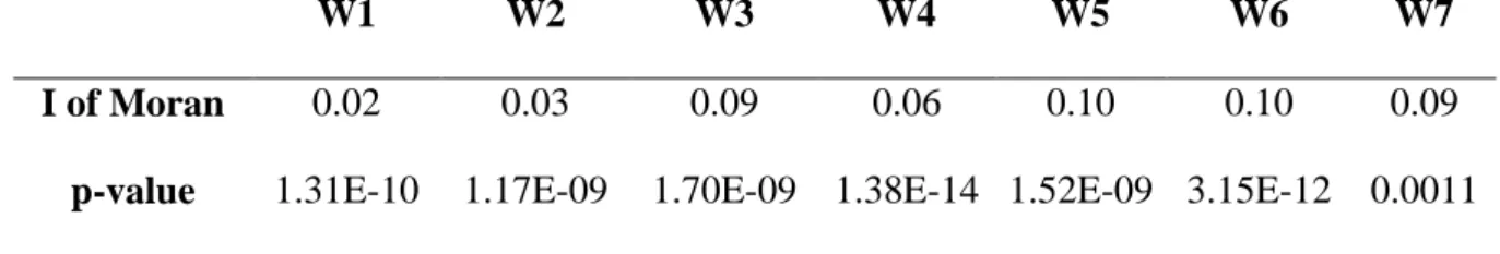
The Moran’s I for the residuals of the OLS model is significantly positive (p-value of 1.31E-10 with W1, see Table A4), highlighting the spatial autocorrelation in our data. Section 4.1 presents the selection of the most suitable spatial models with W1 and section 4.2 presents the estimated parameters of the selected models with W1. We present the robustness checks in section 4.3.
4.1 Selection of the model for the 40 nearest neighbors matrix
Table 2 provides (i) the results for the LM tests for the residuals of the OLS and SLX models, (ii) the goodness-of-fit criteria for the eight models and (iii) the prediction quality criteria for the eight models. The LM tests on OLS residuals indicate that SARAR specification is the most relevant to correct for the spatial autocorrelation of our data when the diffusion of externalities is ignored. With respect to the SLX residuals, the LM tests display the non-significance of the spatial parameters for both the lagged dependent variable and the disturbance term, indicating that it is less appropriate to extend the SLX model to the SDM, the SDEM and the GNS model. This suggest that the spatial interactions on the externalities suites better our data than the
12 Note that the maximum distance between the 40 closer neighbors is 25 kilometers, explaining the setting of the threshold in W4 and W6 to 25 kilometers. However, 75% of the observations present an average distance to the 40th closer neighbor that is less than 10 kilometers, explaining the setting of the threshold in W3 and W5 to 10 kilometers.
23
spatial interactions on price diffusion (captured by SAR and its developments) or on spatial heterogeneity (captured by SEM and its developments).
Table 2: Lagrange Multipliers, goodness-of-fit and prediction quality of the different model specifications with W1
LM test LM test Model R² LL AIC NRMSE
OLS versus SEM (Ho: λ=0) - LM error 20.89*** OLS 0.421 -1101.9 2267.7 76.1
OLS versus SAR (Ho: ρ=0) - LM lag 51.49*** SEM 0.426 -1090.8 2247.6 75.5
OLS versus SARAR (Ho: ρ= λ=0) - LM lag + error 52.43*** SAR 0.430 -1083.2 2232.3 75.4
SLX versus SDEM (Ho: λ=0) - LM error 0.07 SLX 0.447 -1045.1 2214.2 74.3
SLX versus SDM (Ho: ρ=0) - LM lag 2.16E-04 SARAR 0.431 -1081.0 2230.0 75.1
SLX versus GNS (Ho: ρ= λ=0) - LM lag + error 1.17 SDM 0.447 -1045.1 2216.2 74.3
SAR versus SAC (Ho: λ=0) - LM error 2.97° SDEM 0.447 -1045.1 2216.2 74.3
SDM versus GNS (Ho: λ=0) - LM error 1.18 GNS 0.448 -1044.3 2216.5 74.0 ***, **, *, ° stands for p-value of 0.1%, 1%, 5%, and 10% respectively.
The results on the prediction quality of the model indicates that the smallest value of the NRMSE is provided by the GNS specification. Although it is not the smallest value, the NRMSE of the SLX model ranks second with the SDM and SDEM. Similarly, the goodness-of-fit criteria reveal that SLX, SDM, SDEM and GNS specifications improve the estimation quality compared to the OLS, SEM, SAR and SARAR models. The results show that the GNS specification provides the highest R² and maximum likelihood estimation values. However, the results show that the SLX model provides the smallest value of the AIC, i.e., the SLX model minimizes the loss of information. The R² values of the SLX and GNS models are the highest. The tests thus indicate that either the SLX or the GNS models are the best specifications and confirm that the specifications of the spatial diffusion of the externalities capture most of the spatial interactions at stake in our data.
4.2 Spatial hedonic results using the 40 nearest neighbors matrix
Table 3 presents the results of the OLS, SLX and GNS specifications. The structure of the GNS model implies that the estimated coefficients are not the marginal effects. Table 4 summarizes the marginal effects for the SLX and the GNS models. The results on the linear model displays
24
some similar counterintuitive results than those found in the literature. For example, similar to Bontemps et al. (2008), the OLS estimator on temporary grasslands is negative (-0.17). Similar to Le Goffe (2000), we find that the municipal share of cereals increase house prices in the considered municipality (the OLS estimator is 0.16). These two result are counterintuitive but disappear in the SLX and the GNS, once considered the spatial diffusion of the externalities.
25
Table 3: Coefficients for the linear and selected spatial hedonic models with W1
Variables OLS model SLX model GNS model
Est. Coef Std. Err Coef. Std. Err Coef. (lag) Std. Err Coef. Std. Err Coef. (lag) Std. Err
Constant 10.63 0.14 *** 9.70 0,47 *** - - 6,20 1,91 ** - -
Nb_bathroom 0.26 0.02 *** 0.26 0,02 *** 0.11 0.14 0.25 0.02 *** 0.02 0.13
Nb_room 0.11 0.01 *** 0.11 0,01 *** -0.07 0.05 0.11 0.01 *** -0.10 0.04 *
Nb_floor -0.06 0.01 *** -0.06 0,01 *** -0.01 0.10 -0.06 0.01 *** 0.01 0.07
Garden_area 9.41E-06 1.64E-06 *** 9.80E-06 1,23E-06 *** 2.54E-07 1.00E-05 9.79E-06 1.21E-06 *** -3.30E-06 8.25E-06
Oilseeds_area -0.11 0.52 -0.43 0,58 -0.63 2.02 -0.48 0.58 -0.61 1.66 Cereals_area 0.16 0.09 ° -0.34 0,14 * 1.33 0.27 *** -0.33 0.14 * 1.00 0.26 *** Othercrops_area 1.49 3.52 4.33 4,82 -41.26 21.61 ° 4.51 4.80 -33.56 17.95 ° Perm_grassland_area -0.17 0.21 -0.63 0,29 * 1.41 0.61 * -0.58 0.29 * 1.04 0.53 * Temp_grassland area -0.17 0.09 ° -0.51 0,15 *** 0.78 0.32 * -0.52 0.15 *** 0.71 0.27 ** Fallow_area -1.14 3.59 -4.76 4,90 43.29 22.09 ° -4.85 4.87 35.17 18.39 °
Shannon index -4.53E-03 0.06 0.03 0,08 -2.76E-03 0.17 0.04 0.08 -0.02 0.14
Swine_poultry_N -3.62E-04 1.25E-04 ** -6.78E-05 1,43E-04 -8.60E-04 3.58E-04 * -5.86E-05 1.42E-04 -5.60E-04 3.44E-04 °
Cattle_N -8.46E-04 4.06E-04 * -1.13E-03 4,62E-04 * 2.29E-03 1.40E-03 ° -1.14E-03 4.61E-04 * 1.94E-03 1.14E-03 °
D_algae -4.61E-04 1.50E-03 -4.59E-03 0,01 0.01 0.01 -4.47E-03 4.91E-03 0.01 0.01
Ratio_algae -0.13 0.07 ° -0.12 0,12 0.05 0.20 -0.12 0.12 0.10 0.17 Waters_area -0.16 0.81 -3.60E-04 1,12 -1.43 2.22 -0.03 1.11 -1.08 1.84 Wetlands -0.55 0.56 -0.69 0,79 0.74 2.71 -0.65 0.79 0.48 2.24 Shrubs_area 0.37 0.27 0.32 0,35 -0.44 1.03 0.29 0.34 -0.22 0.86 Forest -0.11 0.10 -0.04 0,11 0.04 0.27 -0.04 0.11 0.01 0.22 Greenspace_area 0.29 1.33 -0.32 1,41 -1.23 4.15 -0.06 1.41 -1.31 3.41 Landfills_area 0.56 1.88 -0.49 1,77 5.94 5.78 -0.61 1.77 3.64 4.70 Industries_area 0.25 0.33 -0.22 0,45 -0.93 1.14 -0.30 0.45 -0.65 0.94 Shops_area -0.34 0.22 -0.39 0,26 0.05 0.61 -0.42 0.27 0.29 0.53
D_sea -0.01 1.69E-03 *** 2.29E-04 0,01 -0.01 0.01 -2.00E-04 0.01 -0.01 0.01
D_city -5.93E-04 7.29E-04 -3.55E-03 3,82E-03 3.27E-03 4.30E-03 -4.80E-03 3.63E-03 4.91E-03 4.03E-03
Pop_density 0.02 0.01 ° 0.02 0,01 ° 0.02 0.03 0.02 0.01 ° 0.01 0.03
Revenues 0.03 3.08E-03 *** 0.01 4,69E-03 ** 0.04 0.01 *** 0.01 4.65E-03 ** 0.02 0.01 °
Services 1.77E-04 7.30E-04 1.80E-03 8,00E-04 * -3.97E-03 1.83E-03 * 2.19E-03 8.06E-04 ** -4.17E-03 1.57E-03 **
Time FE Yes Yes Yes
R² 0.421 0.447 0.448
LL -1101.86 -1045.121 -1044.267
AIC 2267.7 2214.241 2216.533
ρ - - 0.358 *
λ - - -0.533 °
26
Indeed, we find in the SLX and GNS models that both the direct and spillover effects of the cereals and the temporary grassland areas are significant. Our results show that they are negatively correlated with the selling prices of the houses within their municipality boundaries but that their spillover effects are positive and higher in absolute term than the direct effects, meaning that they positively influence the utility of the inhabitants living in neighboring municipalities. These results suggest a negative direct effect of temporary grasslands and cereals at the infra-municipal scale, which may be due to short range nuisances (smell, noise, flies associated to grazing cows), but positive local spillovers at the extra-municipal scale, which may be attributed to the landscape attractiveness and amenities. These results are more consistent with the common feeling and stress the utility of the decomposing the effects of agricultural externalities at different scales. We find a similar effect for permanent grasslands, with a negative direct effect and a positive and higher local spillover effects. As permanent grasslands are mainly agricultural wetlands in Brittany, this effect could reflect the local disutility of permanent grasslands due to the presence of flood risk but the positive effects of other externalities, such as biodiversity and landscape beauty, at a larger scale. In the linear model, the result for permanent grasslands was non-significant at the 10% level. This result could indicate that we have disentangled the scale effects of the different externalities by the management of permanent grasslands.