Theoretical and experimental study of tunable liquid crystal lenses : wavefront optimization

(1)

Theoretical and experimental study of tunable liquid

crystal lenses: wavefront optimization

Thèse

Oleksandr Sova

Doctorat en physique

Philosophiæ doctor (Ph. D.)

(2)

Theoretical and experimental study of tunable

liquid crystal lenses: wavefront optimization

Thèse

Oleksandr Sova

Sous la direction de:

(3)

Résumé

Les systèmes optiques adaptatifs ont des applications dans plusieurs domaines: imagerie (zoom et autofocus), médecine (endoscopie, ophtalmologie), réalité virtuelle et réalité augmentée. Les lentilles à base de cristaux liquides font une grande partie de l'industrie de l'optique adaptative parce qu’elles présentent de nombreux avantages par rapport aux méthodes traditionnelles. Malgré les progrès importants réalisés au cours des dernières décennies, certaines limitations de performances et de production existent toujours. Cette thèse explore les moyens de surmonter ces problèmes, en considérant deux types de lentilles adaptatives: lentille à cristaux liquides utilisant le principe de division diélectrique et lentille de contrôle modal.

L’introduction de cette thèse présente la théorie des cristaux liquides et des lentilles adaptatives, abordant également les lentilles à cristaux liquides existantes.

Dans le premier et le deuxième chapitres de cet ouvrage, nous démontrons les résultats de la modélisation théorique de la conception de lentilles à cristaux liquides à double couche diélectrique optiquement cachée. Nous avons étudié l'influence de paramètres géométriques, tels que l'épaisseur de la cellule à cristaux liquides, la forme et les dimensions des diélectriques qui forment la couche optiquement cachée, sur la puissance optique de la lentille. La puissance optique en fonction de la permittivité et de la conductivité relatives des diélectriques a été obtenue. Le comportement d'une telle lentille en présence de variation de température a été analysé.

Nous avons poursuivi la recherche du concept de couche diélectrique cachée en examinant des microstructures basées sur ce principe. Deux systèmes de microlentilles et microprismes ont été simulés. La comparaison de la dépendance de la modulation de phase optique sur la fréquence spatiale des microstructures a été obtenue. Les écarts par rapport aux fronts d'onde idéaux ont été évalués dans les deux cas. Nous avons également comparé les conceptions proposées avec une approche traditionnelle des électrodes interdigitales. Les dispositifs suggérés pourraient être utilisés pour l’orientation de faisceau laser ou comme des réseaux de microlentilles variables.

Dans le troisième et le quatrième chapitres, nous présentons une étude de lentilles adaptatives basées sur le principe de contrôle modal.

Nous avons vérifié les résultats de simulation en les comparant avec les dépendances obtenues expérimentalement de la puissance optique et des aberrations sphériques moyennes quadratiques. Nous avons exploré les modifications suivantes de la lentille de contrôle modal

(4)

traditionnelle: 1) électrode annulaire alimentée supplémentaire; 2) électrode à disque flottant; 3) combinaison des deux premiers cas. L'influence de chaque modification a été étudiée et expliquée. Les résultats des simulations ont montré qu'en utilisant la combinaison d'électrodes supplémentaires avec une technique d'alimentation optimale - le front d'onde pourrait être corrigé à travers la pleine ouverture de la lentille. La lentille modifiée répond aux exigences de faibles aberrations pour les applications ophtalmiques (par exemple, implant intraoculaire).

Finalement, une nouvelle conception d'une lentille de Fresnel de contrôle modal ayant unе grande ouverture a été étudiée. Les performances d'imagerie de la lentille de Fresnel proposée ont été évaluées et comparées à la lentille de référence, construite en utilisant une approche de contrôle modal traditionnelle. Le prototype a démontré l'augmentation de la puissance optique par rapport à une lentille de contrôle modal conventionnelle du même diamètre d'ouverture. Un modèle théorique et des simulations numériques des lentilles de Fresnel ont été présentés. Les simulations ont démontré une possibilité d'amélioration considérable de la qualité d'image obtenue en utilisant des tensions et des fréquences optimisées.

(5)

Summary

Adaptive optical systems have applications in various domains: imaging (zoom and autofocus), medicine (endoscopy, ophthalmology), virtual and augmented reality. Liquid crystal-based lenses have become a big part of adaptive optics industry as they have numerous advantages in comparison with traditional methods. Despite significant progress made over the past decades, certain performance and production limitations still exist. This thesis explores ways of overcoming these problems, considering two types of tunable lenses: liquid crystal lens using dielectric dividing principle and modal control lens.

The introduction of this thesis presents the theory of liquid crystals and adaptive lenses, addressing existing liquid crystal lenses as well.

In the first and second chapters of this work we demonstrate the results of theoretical modeling of double dielectric optically hidden liquid crystal lens design. We have studied the influence of geometrical parameters, such as thickness of liquid crystal cell, shape and dimensions of dielectrics forming the optically hidden layer, on the optical power of the lens. The dependences of optical power on the relative permittivity and conductivity of dielectrics were obtained. The behavior of such a lens in the presence of temperature variation was analyzed.

We have further extended the concept of hidden dielectric layer to exploration of microstructures. Two systems of microlenses and microprisms have been simulated. The comparison of optical phase modulation dependence on spatial frequency of microstructures was obtained. Deviations from ideal wavefronts were evaluated in both cases. We also compared proposed designs with a standard interdigital electrode approach. Suggested devices could be used for continuous light steering or as tunable microlens arrays.

In the third and fourth chapters we present our studies of tunable lenses based on modal control principle.

We verified simulation results by comparing them with experimentally obtained dependences of optical power and root mean square spherical aberrations. We have explored the following modifications of conventional modal control lens: 1) additional powered ring electrode; 2) floating disk electrode; 3) combination of the first two cases. The influence of each modification was studied and explained. Simulation results showed that using the combination of additional electrodes along with optimal powering technique - the wavefront could be corrected within the entire clear aperture

(6)

of the lens. Modified lens meets low aberration requirements for ophthalmic applications (for example, intraocular implant).

Finally, a new design of a wide aperture tunable modal control Fresnel lens was investigated. Imaging performance of the proposed Fresnel lens was evaluated and compared with the reference lens built using traditional modal control approach. The prototype device demonstrated the increase of optical power in comparison with a conventional modal control lens of the same aperture size. A theoretical model and numerical simulations of the Fresnel lens design were presented. Simulations demonstrated a possibility of noticeable image quality improvement obtained using optimized voltages and frequencies.

(7)

List of tables

Table 1.1. Experimental parameters used hereafter as reference for simulations. ... 30

Table 1.2. Comparison of simulations for HCL=185 μm and HCL=92.5 μm. ... 35

Table 1.3. Examples of conductivity values for two different materials. ... 39

Table 1.4. Simulation parameters. ... 40

Table 3.1. Parameter values used for simulations. ... 67

Table 3.2. Optimization parameters and constraints. ... 70

Table 4.2. Optimized control parameters and corresponding calculated OPs. ... 92

(11)

List of figures

Figure I.1. Phase transitions of LCs with the increase of temperature. ... 1

Figure I.2. Three possible deformations of NLC. ... 3

Figure I.3. Molecule of 5CB LC (C18H19N). Color coding for atoms: black – carbon, white- hydrogen, blue – nitrogen. ... 4

Figure I.4. Reorientation of LC molecule with (a) positive and (b) negative dielectric anisotropies in electric field. ... 7

Figure I.5. Schematic representation of LC’s director in Cartesian coordinates. ... 9

Figure I.6. Schematic representation of LC’s director in cylindrical coordinates. ... 11

Figure I.7. Dependence of refractive index encountered by incident beam on director orientation (black arrow – direction of polarization, yellow arrow – direction of propagation). ... 12

Figure I.8. One of the first LC lens designs [22]. ... 14

Figure I.9. GRIN LC lens with a hole-patterned electrode [24]. ... 14

Figure I.10. Schematics of an LC lens with a curved electrode [26]. ... 15

Figure I.11. Scheme of refractive Fresnel lens described in [27]. ... 16

Figure I.12. Schematics of a hidden dielectric double layer lens [28]. ... 18

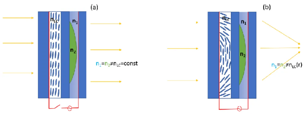
Figure I.13. Schematic demonstration of the hidden layer LC lens with (a) zero control voltage and (b) applied voltage. ... 19

Figure I.14. Geometry of a tunable modal control lens [31]. Dc – diameter of the controlling hole patterned electrode (HPE), WCL – weakly conductive layer, PI – polyimide alignment layer, L – thickness of the LC layer, UTE – uniform transparent electrode. ... 20

Figure I.15. Equivalent electric circuit of the MC lens [31]. ... 21

Figure 1.1. Schematic of the DDOH layer lens [30]. ... 27

Figure 1.2. Schematic of the dielectric divider concept. ... 27

Figure 1.3. Example of experimentally measured dependence of OP of the lens versus the applied RMS voltage. Uth, Umin, and Umax are the threshold, minimum, and maximum considered voltages, respectively. ... 28

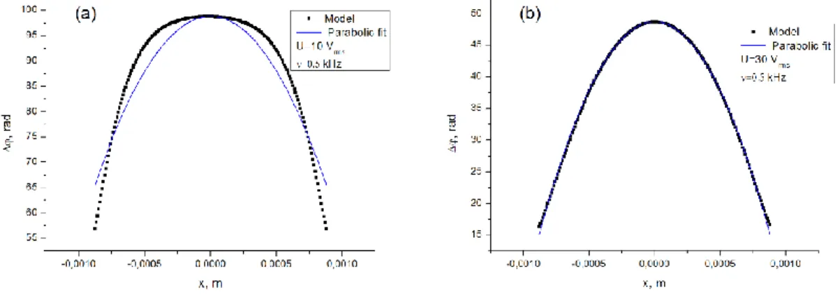
Figure 1.4. Parabolic approximation of optical phase retardation. Control voltage was (a) 10 Vrms and (b) 30 Vrms. ... 31

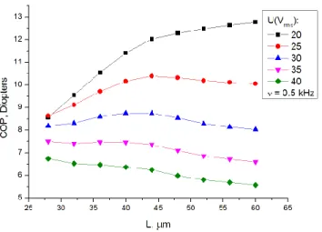
Figure 1.5. COP as a function of LC cell thickness and driving voltage. ... 32

Figure 1.6. Schematics of the double dielectric hidden layer... 34

Figure 1.7. OP dependence on changes of the height HCL of the CL (varied from 50% to 300% of the experimental value). ... 36

Figure 1.8. Variation of the base radius of the CL. ... 36

Figure 1.9. OP versus base radius of the CL. ... 37

Figure 1.10. OP dependence on the relative permittivity of index matching layer. The relative permittivity of the CL was fixed to 3.9. ... 38

Figure 1.11. OP dependence on the conductivity of index matching layer. Relative permittivity is the same for CL and IML. Conductivity of CL was constant: σCL=1∙10-13 S/m. ... 39

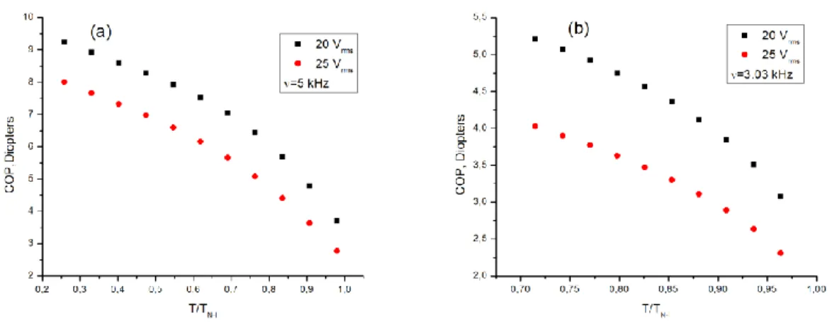
Figure 1.12. Temperature dependence of OP for (a) E49 and (b) 5CB LCs. Nematic-isotropic transition temperatures (TN−I) for E49 and 5CB were about 97°C and 35.1°C, respectively. ... 40

Figure 2.1. Schematics of the simulated microlens array with sinusoidal distribution of the CL material. ... 47

Figure 2.2. Optical power dependence on control voltage (single LC lens), for different thicknesses of middle glass substrate (aperture diameter = 1.75 mm). ... 47

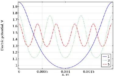
Figure 2.3. Electric potential distribution in the middle of the LC cell for different numbers of microlenses within 2000 μm wide simulated system (different spatial frequencies). ... 48

Figure 2.4. Modulation transfer function (the case of sinusoidal CL material). ... 49

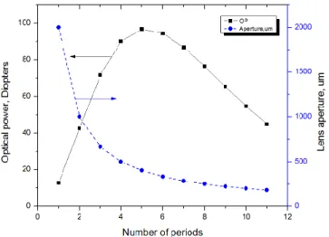
Figure 2.5. Dependence of the optical power and lens aperture diameter of each microlens versus the number of CL units (the case of sinusoidal CL material). ... 50

(12)

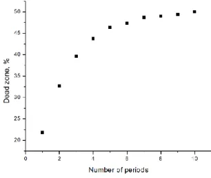
Figure 2.6. Normalized RMS phase retardation deviation from ideal parabolic shape and difference between max and min phase retardation (the case of sinusoidal CL material) versus the number of CL units. ... 50 Figure 2.7. Schematics of the simulated microprism array. ... 51 Figure 2.8. Electric potential distribution in the middle of the LC cell for different numbers of microprisms within 2000 μm wide simulated system (different spatial frequencies). ... 51 Figure 2.9. Modulation transfer function (the case of microprism array). ... 52 Figure 2.10. (a) Director tilt angle in the middle of the LC cell for 1, 3 and 5 microprisms over 2000 μm and (b) the corresponding phase shifts. ... 52 Figure 2.11. Percentage of the prism width in the “dead zone” due to fringing fields versus the number of microprisms per 2000 μm. ... 53 Figure 2.12. Normalized RMS phase retardation deviation from the (desired) linear form and the difference between max and min phase retardation values versus the number of microprisms over 2000 μm within the (a) “active zone” of single microprism and (b) in the entire clear aperture of the microprism (covering both active and passive zones). ... 54 Figure 2.13. Schematics of the “out of plane” switching. ... 55 Figure 2.14. Modulation transfer function (the case of “out of plane” switching using patterned electrodes).

... 55 Figure 2.15. Optical power of each microlens depending upon the gap between two neighboring electrodes (the case of “out of plane” switching using patterned electrodes). ... 56 Figure 2.16. Normalized RMS phase retardation deviation from ideal parabolic shape and difference between max and min phase retardation (the case of “out of plane” switching using patterned electrodes). ... 56 Figure 3.1. Conventional modal control LC lens design, WCL – weakly conductive layer, HPE – hole patterned electrode, UTE – uniform transparent electrode, LC – liquid crystal of thickness L. ... 62 Figure 3.2. Simulated wavefront generated by a standard modal control lens (black solid line) versus the ideal parabolic fit (blue dashed line). r = 0 is the center of the lens, while r =1.5 mm is its periphery. ... 62 Figure 3.3. Schematic representation of the experimental setup used for measuring the OPs and SAs of TLCLs: 1) He-Ne laser, 2) polarizers, 3) beam expander, 4) function generator, 5) TLCL, 6) relay lens, 7) Shack-Hartmann wavefront sensor. ... 65 Figure 3.4. Experimentally measured dependences of real and imaginary relative permittivities (parallel and perpendicular components) of LC material upon applied signal’s frequency. ... 66 Figure 3.5. (a) Comparison of simulated (open circles) and measured (filled squares) dependences of the OP of the standard modal control TLCL upon the driving frequency. (b) Comparison of corresponding RMS spherical aberrations vs frequency. Applied voltage is 5 Vrms. The clear aperture is 3 mm. ... 67 Figure 3.6. Schematics of modified modal control lens designs. (a) MC lens with inner ring electrode (Din.r. – diameter of the inner ring electrode); (b) MC lens with a floating electrode (Dfl.el. – diameter of the floating electrode); (c) a design combining components of (a) and (b). ... 68 Figure 3.7. Optical power (filled squares) and RMS SAs (open circles) simulated for a standard modal control lens with 4 mm clear aperture. ... 69 Figure 3.8. Comparison of RMS spherical aberrations vs optical power for different designs of optimized MC lenses: (a) MC; (b) MC+inner ring; (c) MC+floating electrode; (d) MC+inner ring+floating electrode. ... 71 Figure 3.9. (I) Normalized wavefronts and (II) deviations of phase retardation from the ideal shape: (a) MC; (b) MC+inner ring; (c) MC+floating electrode; (d) MC+inner ring+floating electrode. 72 Figure 3.10. RMS SAs of optimized lens with combined additional electrodes. ... 73 Figure 4.1. Schematic presentation (a) and top substrate electrode pattern (b) of the studied Fresnel lens; WCL - weakly conductive layer, CRE – concentric ring electrodes, UTE - uniform transparent electrode, LC – liquid crystal. ... 79

(13)

Figure 4.2. Observed interference fringes obtained with the F-MC-TLCL placed between crossed polarizers. Green dashed lines separate inner and outer zones. U = 4 Vrms, (a) f=10 kHz, U1=0.35

Vrms; (b) f=10 kHz, U1=2 Vrms; (c) f=20 kHz, U1=0.35 Vrms; (d) f=20 kHz, U1=2 Vrms. ... 81

Figure 4.3. Reconstructed phase profiles for the proposed F-MC-TLCL. Dashed lines are for eye guiding only. ... 81 Figure 4.4. Optical characterization for the reference (classic MC-TLCL) and the proposed here (F-MC-TLCL) lenses. (a) OP vs frequency, (b) RMS wavefront errors vs frequency. Solid lines are third order polynomial approximations used for eye guiding only. ... 82 Figure 4.5. Schematics of the experimental setup used for comparison of image quality between MC-TLCL and MC-TLCL: (1) raspberry pi v4 [100], (2) raspberry pi camera v2 [101], (3) F-MC-TLCL or MC-F-MC-TLCL, (4) polarizer, (5) USAF resolution chart, (6) function generators. ... 83 Figure 4.6. Pictures of the USAF resolution chart recorded by using the raspberry pi camera with (a) conventional MC-TLCL (unpowered); (b) MC-TLCL with U=3 Vrms, f=22.5 kHz; (c) F-MC-TLCL with U=4 Vrms, U1=0.35 Vrms, f=22.5 kHz. The small horizontal red line (in the centers of pictures)

is used for intensity scan and analyses (see Fig. 4.7). ... 84 Figure 4.7. Contrast plots (a) conventional MC-TLCL (unpowered); (b) MC-TLCL with U=3 Vrms, f=22.5 kHz; (c) F-MC-TLCL with U=4 Vrms, U1=0.35 Vrms, f=22.5 kHz. ... 85

Figure 4.8. Picture of a target with increasing spatial frequency (in lp/mm) (a) without TLCL, when the raspberry pi camera is focused to infinity; (b) using MC-TLCL with U=3 Vrms, f= 22.5 kHz; (c) using F-MC-TLCL with U=4 Vrms, U1=0.35 Vrms, f= 22.5 kHz. Blue horizontal lines are used for

following intensity scans (see Fig. 4.9). ... 85 Figure 4.9. Contrast comparison for various spatial frequencies along the blue horizontal line (see Fig. 4.8) without TLCL, raspberry pi camera is focused to infinity (dashed blue line with circles); using conventional MC-TLCL (red dashed line with triangles) and F-MC-TLCL (black solid line). ... 86 Figure 4.10. Pictures of objects taken with raspberry pi camera focused to infinity (a) without TLCL, (b) MC-TLCL with U=3 Vrms, f= 22.5 kHz; (c) F-MC-TLCL with U=4 Vrms, U1=0.35 Vrms, f= 22.5

kHz; (d) – solid lines are gray values measured along red lines shown in (a)–(c), lines with symbols are corresponding Gaussian fits. ... 87 Figure 4.11. Experimental measurements of 5CB’s real and imaginary relative permittivity components at different applied signal’s frequencies. ... 89 Figure 4.12. Comparison of (a) OPs and (b) RMS aberrations (total RMS wavefront errors in case of experiment and RMS SAs in case of theory) between experimentally acquired data and results obtained through simulations with fitting parameters. ... 90 Figure 4.13. RMS wavefront errors vs OPs. Experimental results for MC-TLCL (U=3 Vrms) – black line with squares, experimental result for F-MC-TLCL (U=4 Vrms, U1=0.35 Vrms) – red line with

circles, simulation of F-MC-TLCL (U=4 Vrms, U1eff=1.61 Vrms ) – blue line with up triangles,

simulation of F-MC-TLCL (optimized driving) – green line with down triangles. ... 91 Figure 4.14. Wavefront comparisons (a) and processed wavefronts (b) with parabolic approximations (solid lines): experimentally obtained wavefront for F-MC-TLCL (U=4 Vrms, U1=0.35 Vrms, f=22.5

kHz) – black line with squares; simulated F-MC-TLCL (U=4 Vrms, U1eff=1.61 Vrms, f=22.5 kHz) –

red line with circles; simulated F-MC-TLCL (optimized driving) – blue line with triangles. ... 92 Figure B.1. Schematics of light propagation through LC lens. ... 98 Figure B.2. Point spread function of simulated modal control lenses with 4 mm clear aperture: (a) – traditional approach, (b) – modified lens with improved aberrations. ... 99 Figure B.3. Modulation transfer function of simulated modal control lenses with 4 mm clear aperture: (a) – traditional approach, (b) – modified lens with improved aberrations. ... 99 Figure B.4. Simulated phase profiles of microprisms (orange dashed lines) and corresponding ideal profiles (blue solid lines) in the case of (a) 1 prism over 2000 μm and (b) 3 prisms over 2000 μm. ... 100

(14)

Figure B.5. Light intensity distribution (arbitrary units) along direction of beam propagation (z axis), simulated using (a) ideal prism phase retardation profile, (b) phase retardation profile of a microprism with the “dead zone”. Spatial frequency of the hidden dielectric structure is 1 microprism over 2000 μm (see Fig. B.4 (a)). ... 100 Figure B.6. Light intensity distribution (arbitrary units) along direction of beam propagation (z axis), simulated using (a) ideal prisms’ phase retardation profile, (b) phase retardation profile of microprisms with the “dead zone”. Spatial frequency of the hidden dielectric structure is 3 microprisms over 2000 μm (see Fig. B.4 (b)). ... 101

(15)

(16)

Acknowledgments

Firstly, I would like to thank Professor Tigran Galstian for giving me an opportunity to do my doctoral studies at Laval University. I want to express my gratitude for all discussions, comments and advices that I have received from him working on different projects. He has provided enormous help and support during my research. Without his guidance and encouragement this thesis would not have been possible.

I would also like to thank the Theoretical Physics Department of Taras Shevchenko National University of Kyiv. I am particularly grateful to Professor Victor Reshetnyak, who has introduced me to the world of liquid crystals and constantly supported me on my scientific journey.

I thank the R&D group of LensVector Inc. for the use of their equipment, discussions and technical advices.

I would like to thank Professor Michel Piché for reviewing the present thesis before submission. His valuable remarks and comments have helped to increase the quality of this work.

I want to thank the administrative and technical staff of COPL and Laval University for providing all necessary services, permitting me to conduct my research. Particularly, I want to thank Patrick Larochelle and Souleymane Toubou Bah who have always found ways to resolve any issues in laboratories.

I thank the Sentinel North of NSERC/Laval University for their financial support.

Thanks to my family in Ukraine and friends (all over the world) who have welcomed my decision to move to Canada to continue my studies and helped me to integrate into Quebec society. I would like to express special thanks to my wife who has been by my side every step of this PhD project.

(17)

Foreword

This thesis is based on four articles published in peer-reviewed journals. I am the principal author in all the articles that were inserted in the thesis.

The thesis begins with an introduction into theory of liquid crystals. All numerical models presented further in this thesis were constructed within the theoretical framework described in the introduction.

An overview of existing tunable liquid crystal lens designs is presented. Their advantages and drawbacks are discussed referring to publications. The designs explored in this PhD project are briefly introduced.

The first chapter consists of an article discussing design and theoretical analyses of controllable liquid crystal lenses that use optically hidden dielectric double layer. The second chapter studies a possibility to extend the concept of hidden dielectric layer to construction of tunable microlens and microprism arrays. These articles were co-authored by Professor Victor Reshetnyak from Taras Shevchenko National University of Kyiv:

• O. Sova, V. Reshetnyak, T. Galstian, Theoretical analyses of a liquid crystal adaptive lens with optically hidden dielectric double layer, J. Opt. Soc. Am. A. 34 (2017) 424–431. • O. Sova, V. Reshetnyak, T. Galstian, Modulation transfer function of liquid crystal

microlenses and microprisms using double dielectric layer, Appl. Opt. 57 (2018) 18–24. All authors participated in the discussion and manuscript writing. Simulation results presented in these articles were obtained by me.

The third and fourth chapters discuss tunable lenses based on modal control. In the third chapter we present the theory of modal control lenses. We verify the results of numerical simulations by comparing them with experimental data. Then we suggest several design modifications that help to improve image quality provided by these lenses. In the fourth chapter we present an article in which we introduce a new design of a wide aperture tunable modal control Fresnel lens. The experimental procedure is discussed. Comparison of experimental measurements of the Fresnel lens with a conventional reference lens is performed and analyzed. A theoretical model and optimization strategy are presented.

• O. Sova, T. Galstian, Liquid crystal lens with optimized wavefront across the entire clear aperture, Opt. Commun. 433 (2019) 290–296.

(18)

• O. Sova, T. Galstian, Modal control refractive Fresnel lens with uniform liquid crystal layer, Opt. Commun. 474 (2020) 126056

Experiments and designs were discussed with Professor Tigran Galstian. Sample preparations, experimental measurements and theoretical simulations were realized by me. The manuscripts were written under supervision of Professor Tigran Galstian. I provided my versions of the manuscripts which then were completed in accordance with Professor Galstian’s edits and recommendations.

Co-authors:

Tigran Galstian: Center for Optics, Photonics and Laser, Department of Physics, Engineering Physics and Optics, Laval University, Pav. d’Optique-Photonique, 2375 Rue de la Terrasse, Québec, G1V 0A6, Canada.

e-mail: galstian@phy.ulaval.ca

Victor Reshetnyak: Theoretical Physics Department, Taras Shevchenko National University of Kyiv, Volodymyrska street 64, Kyiv, 01601, Ukraine.

e-mail: VReshetnyak@univ.kiev.ua

Publications during PhD program:

1. O. Sova, V. Reshetnyak, T. Galstian, Theoretical analyses of a liquid crystal adaptive lens with optically hidden dielectric double layer, J. Opt. Soc. Am. A. 34 (2017) 424–431. 2. T. Galstian, O. Sova, K. Asatryan, V. Presniakov, A. Zohrabyan, M. Evensen, Optical

camera with liquid crystal autofocus lens, Opt. Express. 25 (2017) 29945–29964.

3. O. Sova, V. Reshetnyak, T. Galstian, Modulation transfer function of liquid crystal microlenses and microprisms using double dielectric layer, Appl. Opt. 57 (2018) 18–24. 4. O. Sova, T. Galstian, Liquid crystal lens with optimized wavefront across the entire clear

aperture, Opt. Commun. 433 (2019) 290–296.

5. O. Sova, T. Galstian, Modal control refractive Fresnel lens with uniform liquid crystal layer, Opt. Commun. 474 (2020) 126056

Conference presentations

1. O. Sova, T. Galstian, Modal liquid crystal lens with optimized wavefront control, Photonics North, Montreal, June 5-7, 2018.

(19)

2. O. Sova, T. Galstian, Refractive modal control liquid crystal Fresnel lens, Sentinel North Scientific Meeting, Lévis, August 26-28, 2019

3. O. Sova, T. Galstian, Refractive modal control liquid crystal Fresnel lens, OLC 2019, Quebec, September 8-13, 2019

(20)

Introduction

I.1 Types of liquid crystals: nematics, smectics, cholesterics

Liquid crystalline state of matter has been discovered in the 19th_{century. In the state of} mesophase, liquid crystals (LCs) possess properties of both liquids (molecular flow) and crystals (optical, dielectric, diamagnetic anisotropies). In order to characterize LCs, a unit vector, called the director n(r), that shows the average orientation of long molecular axes of LC molecules at a certain position in space was introduced [1]. It should be noticed that n and -n states are identical. The first classifications of LCs were made based on director’s orientation relative to the centers of mass of molecules. Generally, LCs are divided into two main groups: thermotropic and lyotropic. For thermotropic LCs, mesophase exits only in a certain range of temperatures, when for lyotropic LCs it depends on the concentration of amphiphilic molecules [2]. Further in this thesis we will discuss only thermotropic LCs.

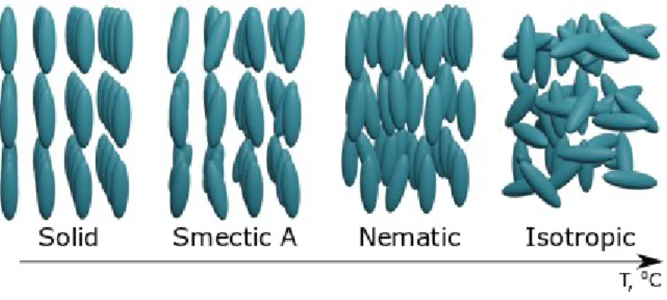
Thermotropic LCs can be subdivided into several types: nematic, smectic and cholesteric. Some LCs can transition from one mesophase to another with the increase of temperature. These possible phase changes as a function of temperature are demonstrated in Figure I.1:

Figure I.1. Phase transitions of LCs with the increase of temperature.

Nematic LCs (NLC) have molecules that are elongated in one direction. The centers of mass of these molecules are distributed in space chaotically [3]. Therefore, no positional, but only long-range orientational order is present in nematics. Their molecules can be approximated with rods or cylinders. It is one of the most common liquid crystalline phases. The molecules can be oriented with external electric or magnetic fields (as a consequence of anisotropy, see hereafter). Uniformly oriented samples are optically uniaxial and strongly birefringent [2]. Nematics have found numerous

(21)

applications is modern commercial technologies such as displays [4], beam steering devices [5], tunable lenses [6].

Smectic LCs have well defined layers of molecules. This mesophase is observed at lower temperatures than nematic one and has higher degree of order. Molecular structure of smectics resembles a two-dimensional crystal, where in each layer the molecules are oriented at a certain angle relative to layer’s surface. Layers can slide freely over each other as interlayer forces are week in comparison with lateral forces between molecules in each layer [2].

Cholesteric mesophase possesses higher symmetry in comparison with nematics. It is composed of optically active molecules that gradually change their orientation, rotate around the axis normal to director. This twist can be either left- or right-handed depending on molecular structure. The distance at which molecules make one full rotation around the axis is called a chiral pitch. The pitch can be varied with temperature or by adding other molecules.

Although cholesteric and smectic LCs are interesting from scientific research and commercial device production sides (reflective cholesteric display [7], light shutters [8]), our work is based on investigation of nematics.

I.2 Continuum theory of liquid crystals

To give a theoretical description of phenomena observed in LCs we need a parameter that characterizes long-range orientational order. The director gives only qualitative characterization of molecular orientation and does not depict the influence of external electric field, mechanical deformations, or temperature [3]. Therefore, the use of director alone for LC characterization becomes insufficient. Thus, we define an order parameter, which is a second rank tensor as follows [1]:

1 ( )

,

3 Q

_

=

Q T n n



_

_{ }

−



_



_





(I.1)

where Q(T) – temperature dependent scalar order parameter; nα, nβ – director components, δαβ -

Kronecker delta. In the case of isotropic liquids Q(T) = 0, for solids its value becomes 1 and for all known nematic phases 0<Q(T)<1 [9,10].

It is convenient to consider LC as a continuous medium, disregarding the processes that take place on molecular scale [1,11]. This approach is justified when the following conditions are fulfilled [12]:

(22)

1) The energy of intermolecular interactions is much higher than given energy per molecule participating in physical processes

2) Involved characteristic distances (where we can observe significant variations of Qαβ) for

these phenomena are larger (~1 um) than molecular dimensions (~ 20 A) [1]

Developed by Oseen [13] and Frank [14] continuum theory can successfully describe the behavior of LCs in the presence of external (electric or magnetic) fields as well as orientational effects coming from bounding substrates.

Equilibrium state of LCs corresponds to a minimum of free energy. Deviation from this state comes with additional energy related to LC deformations [3]. We can construct the expression for free energy density, developing it into series of tensor order parameter and its gradients (corresponding to energy distortions). Because tensor Qαβ varies at much larger distances than

molecular size - the distorted state of nematics can be described in terms of n(r). The director is assumed to vary slowly and smoothly within the volume of LCs.

We distinguish three main types of deformations of NLCs due to the influence of external fields (electric or magnetic). They are called splay, twist and bend (Fig. I.2).

Figure I.2. Three possible deformations of NLC.

Frank and Oseen have suggested an expression describing the contributions of each basic deformation into total free energy density:

2 2 2 2 3 11 2 3

1

1 (

)

(

)

(

)

2

2 ,

2 K

K

f

=



n

+

n

 

n

dV

+

K

n

 

n

(I.2)

where K11, K22, K33 are splay, twist and bend elastic constants respectively (terms used by analogy

(23)

3 2 2 2 2 11 2 3 1 1 1 ( ) ( ) ( ) . 2 2 2 elastic F = K

_

n dV + K

_

n n dV + K

_

n  n dV (I.3)

This expression is the fundamental equation of the elastic continuum theory of nematics [12]. Further we will use it to describe the response of LC molecules to the presence of electric field.

I.3 Dielectric and optical anisotropies of liquid crystals

The molecules of LCs have various forms (for example disc shaped or banana-shaped) that define their physical properties. We will discuss nematic molecules that are elongated in one direction. The molecular conformation of a typical NLC 5CB is shown in Figure I.3.

Figure I.3. Molecule of 5CB LC (C18H19N). Color coding for atoms: black – carbon, white- hydrogen, blue – nitrogen.

In practice, LC mixtures are often used (for example E49 or E7 which contains multiple components: C18H19N, C20H23N, C21H25NO, C24H23N). LC molecules are mostly composed of neutral atoms. But bonds between atoms lead to one part of the molecule to possess a positive charge when the other part possesses a negative charge. Thus, these molecules are permanent dipoles. The situation when molecules are electrically neutral, but in the presence of electric field the charges inside them are displaced (induced dipole) is also possible [15]. As the result of dipole moment present in NLCs, their orientation can be controlled with application of electric field (this will be discussed in detail in section I.4).

Liquid crystals exhibit anisotropic properties due to their molecular structure. Dielectric constants measured along (ε∥) long molecular axis and perpendicular to it (ε⊥) have significantly different values. Dielectric anisotropy of an LC is defined as εa= ε∥-ε⊥. In contrast with isotropic materials, the dielectric permittivity of LCs is not a constant, but a second rank tensor. To describe the propagation of light in liquid crystals we further consider them to be electrically anisotropic, non-conductive and magnetically isotropic. Strictly speaking, LCs have magnetic anisotropy χa= χ∥-χ⊥

(24)

(where χ∥ and χ⊥ are magnetic susceptibilities measured along and perpendicular to director, respectively), but χa<<1 and hence magnetic permeability μ≈1 [10,16].

To consider propagation of light in anisotropic medium we start with Maxwell’s equations for electric and magnetic fields. In this section we use Gaussian convention. In the absence of free charges and currents, Maxwell’s equations take the following form:

0

1

0

1 0,

c t

  =



 +

=



 −

=



D

B

E

D

H

(I.4) (I.5) (I.6) (I.7) where c is the speed of light, E – electric field vector, H – magnetic field vector, B – magnetic induction vector, D – dielectric displacement vector.

The solutions for electric and magnetic fields are plane monochromatic waves:

( ) ( )_. i t i t e e   − − = = kr 0 kr 0 E E H H (I.8) (I.9) Substituting Equations (I.8), (I.9) into Equations (I.6), (I.7) and introducing a unit vector

k

=

k

s

, where k c n 

= , Equations (I.6), (I.7) transform into (I.10) and (I.11) correspondingly:

,

[

]

[

]

n





=

= −

s E

H

s H

D

(I.10) (I.11) where constitutive relation B =Hhas been used.

Excluding H from Equations (I.10) and (I.11), we can rewrite (I.11) as 2

(

)).

n



=

−



D

E s s E

(I.12)

As mentioned above, dielectric permittivity in anisotropic materials is a tensor. Given the fact that this tensor is symmetric, we can choose a coordinate system where it would have only diagonal components:

0

0 ˆ

0 0 .

0

x y z











= 











(I.13)

(25)

Then Equation (I.12) takes the following form (where E is now E=E0ei(kr)_):

2

₍

_)),

_{, , .}

i i

E

n E s

i i

i x y z



=

−

s E



=

(I.14)

Performing a series of simple mathematical transformations using Equation (I.14) that are described in [17], we obtain Fresnel’s equation of wave normals:

2

₍

2 2

₎₍

2 2

₎

2

₍

2 2

₎₍

2 2

₎

2

₍

2 2

₎₍

2 2

_{) 0,}

y z p y z x p p p x z p x p y

s

   

−

+

s

   

−

+

s

   

−

=

(I.15) where _p c n  = - phase velocity, i i

c





=

(i=x, y, z) - principal velocities of propagation.

Further we will consider only optically uniaxial crystals (



_o

=



_x

=



_y,

 

_e

=

_z) as this represents the case of NLC. Defining the angle between z axis and vector s (parallel to k) to be θ, Equation (I.15) becomes:

2 2 2 2 2 2 2 2

(

 

_p

−

_o

)[(

 

_p

−

_e

)sin



+

(



_p

−



_o

)cos



]

=

0.

(I.16) This quadratic equation has two solutions for



_p2:

2 2 1 2 2 2 2 2 2

cos

sin

.

o o e p p









=

+

(I.17) (I.18) Finally, these solutions can be rewritten in terms of refractive indices as follows:

1 2 ₂ ₂o ₂ ₂

.

e o o e

c

n

os

n

si

n



=

+

=

_(I.19) (I.20) Therefore, in the anisotropic media, such as NLC, we can observe two propagating waves: the ordinary wave encounters the ordinary refractive index, which is independent of direction of propagation; the extraordinary wave encounters an effective refractive index that changes as a function of angle between wave vector and optical axis.

I.4 Liquid crystals in the presence of external electric field

The orientation of LC molecules changes under the influence of external electric or magnetic fields. We will discuss the case of electric field as it is used for most practical applications. The energy that comes from the contribution of electric field:

) 1 dV, 2 ( E F =−

_

E D (I.21)

(26)

where

D

=

 

₀

ˆ

E

is dielectric displacement vector, ˆ- dielectric tensor. Then the whole expression for free energy becomes

2 22 33 2 2 11

1

1 (

)

(

)

(

)

,

2

2 (

)

dV

elas ict E

F F

F

dV

K



K



K



=

+ =



=



n

+



n

+



n

−



E D



(I.22)

Dielectric tensor depends on director components as follows:

.

ˆ

_ij _{a i}

n n

_j

  

=

_⊥

+



(I.23)

Dictated by the chemical structure of LC molecules, dielectric anisotropy εa (see page 4) can be either positive, as shown in Figure I.4 (a), (ε∥>ε⊥) or negative, Figure I.4 (b), (ε∥<ε⊥).

Figure I.4. Reorientation of LC molecule with (a) positive and (b) negative dielectric anisotropies in electric field.

NLCs with positive dielectric anisotropy have their dipole moments directed parallel to long molecular axis. Therefore, these molecules tend to change their orientation to be parallel to the external electric field, as this state is energetically preferable. On the other hand, NLCs with negative dielectric anisotropy (which is typical for molecules that are permanent dipoles) have dipole moments perpendicular to long molecular axis. In this case they change their orientation in such a way that director is perpendicular to electric field. In this thesis we work with NLCs that have positive dielectric anisotropy.

Let us discuss a simple case of electric field induced reorientation of NLC with positive dielectric anisotropy in a planar cell. Under the condition that LC molecules are initially completely parallel to cell substrates, there exists a threshold voltage at which molecules start changing their orientation [1]:

(27)

11 33 0 ) / ( . 2 th a K K V



 

+ = (I.24)

This process is called a Frederiks transition and was originally observed in a meniscus (formed by a plane glass and a convex glass) in magnetic field, but the equivalent effect also takes place in electric field. We see that Vth is independent of cell geometry and is a function of elastic and

dielectric properties of LC. For V>>Vth the molecules become completely reoriented, with their dipole

moments being parallel to the electric field. Usually the AC voltage is applied, as in DC voltage we observe the migration of charged particles to one electrode of the cell structure, damaging it eventually. Thin transparent layers of conductive materials (for example indium-tin-oxide, ITO) are deposited on glass substrates to serve as electrodes. The thickness of ITO layer is about 20 - 50 nm.

Equation (I.22) shows that there are two competing sources contributing into free energy. Elastic forces tend to keep the molecules oriented in accordance with initial, non-disturbed state. On the other side, electric field forces tend to orient the molecules to align them parallel to E. Inner surfaces of LC cells are usually covered with polyamide, that is mechanically rubbed or chemically treated to create grooves. They provide nearly parallel orientation of molecules in proximity to glass substrates (planar initial orientation), defining distribution of director within the cell. Some types of polyamides make molecules nearly perpendicular to contact surfaces (homeotropic orientation).

From the point of view of electric circuits, an LC cell can be represented as a leaky variable capacitor with capacitance gradually changing from C⊥=ε0ε⊥S/d when the cell is unpowered to

Cǁ=ε0εǁS/d for a cell where LC is completely reoriented, where ε0 – dielectric permittivity of vacuum, S – cell area, d – cell thickness.

It should be mentioned that dielectric constants of LCs are frequency dependent. For many mobile applications, the typical working frequency does not exceed several kHz (as it is directly proportional to power consumption), but in certain cases the use of higher frequencies is justified. An example of such a system will be presented further.

When the electric tension is switched off – a relaxation of molecules occurs, as they return to the state of original orientation. The times of molecular relaxation and excitation can be evaluated as [18]: 2 1 2 , relax L K







= (I.25)

(28)

2

,

1

relax excit th

V



=





−









(I.26)

where γ1 is rotational viscosity of LC, K – elastic constant (K≈K11≈K33 – one constant approximation).

Dielectric and optical anisotropies of LCs as well as simple means of orientational control are widely exploited in modern optical technology. In the next section we will demonstrate the governing equations for LC reorientation within the frame of continuum theory, based on the full free energy described by Eq. (I.22).

I.5 Partial differential equations describing the reorientation of molecules

Having built free energy functional (Eq. (I.22)) we can now search for such a distribution of LC molecules under the influence of electric field, that results in a steady state. Mathematically, this is the problem of variational calculus [19], where free energy is a functional to be minimized. Finding the first variation and equalizing it to zero, we obtain the Euler-Lagrange equation. The solution of this partial differential equation (PDE) is a function that corresponds to minimum of free energy and therefore is a steady state distribution. Let us present several geometries that will be used further in this thesis.

We start with a geometry shown in Figure I.5, considering Cartesian coordinate system:

Figure I.5. Schematic representation of LC’s director in Cartesian coordinates.

where the LC cell is assumed to be infinitely long in y direction. Thus, the reorientation of LC molecules takes place in xOz plane. This assumption is often made to simplify PDE, as resulting

(29)

solutions still agree well with experiments. The angle between director n(r) and x axis is θ, then director components are the following:

(cos ,0,sin ).



=

n

(I.27)

Then the resulting PDE for director’s reorientation angle is

(

)

2 2 2 2 11 33 11 33 2 2 33 11 2 2 0

(

sin

cos

)

(

cos

s

)

E

in

)sin

sin 2

sin

E cos 2

0,

(

) (

cos

cos (

E ) E

xx zz z x xz a z x x z

K



 



 











−

+

_

+

_

+

−

+

=

(I.28)

where ε0 is the dielectric constant of vacuum, θxx= ∂2θ/∂x2, θxz= ∂2θ/∂x∂z, Ex=∂E/∂x.

This PDE should be accompanied by boundary conditions for θ (at z=0 and z=L). We use strong anchoring approximation, meaning that LC’s director can not deviate from a certain predefined orientation at boundary surfaces θ(x,0)=θ(x,L)=θ1. For planar orientation, the value of θ1 is several degrees. A different approach, that can often be found in literature, is called weak anchoring boundary condition. In this case, one more term (for example an expression proposed by Rapini and Papoular [20]), describing surface anchoring energy should be added to total free energy. Then boundary conditions would take more complex form.

A one elastic constant approximation, meaning that K11=K33=K, is widely used to simplify PDE (I.28). Under this condition, Equation (I.28) is transformed into

(

2 2

)

0

_.

(

)

a

sin

co

s (E

E

) E

E

cos

2

0

xx zz z x x z

K





+



+





−

+



=

(I.29)

When LC cell’s dimension in x direction is much larger than its height (which in many cases holds true), all x derivatives and Ex field component become small and can be neglected; then Equation (I.29) further simplifies to

(

2

)

0 a

_sin

_{cos (E}

₎

_0.

zz z

K





+





=

(I.30)

The other geometry used in our projects consists of a cell with top annular electrode and bottom whole transparent electrode. Given the symmetry, the choice of a cylindrical coordinate system is more suitable (Fig. I.6):

(30)

Figure I.6. Schematic representation of LC’s director in cylindrical coordinates.

Director angle does not change with rotation around z axis. Applying similar procedure of variational calculus and one constant approximation, we obtain the following equation:

(

2 2

)

0 a

_sin

_cos

_(E

_{E )}

_E

_{cos 2}

₀

_.

zz

_K

z z    













+

−

+

=

(I.31)

Typically, the diameter of top ring electrode is much larger than cell’s height. Thus, neglecting ρ derivatives and Eρ electric field component, we can simplify (I.31) to the form similar to Equation (I.30).

Having chosen the appropriate equation for director reorientation (either (I.30) or (I.28), for the problems that we worked on), we needed to couple it with Maxwell’s equations. Considering only the influence of electric field and assuming no free charges present in LC, Maxwell’s equations simplify to the equation for electric potential:

0

ˆ

i

V

0,



 









_

+

_



_

=









(I.32)

where ˆ is a dielectric tensor as given by Equation (I.23). Boundary conditions for this equation are chosen individually for each problem, corresponding to the applied control voltage.

The system of coupled PDEs for director reorientation and electric field distributions are solved numerically using finite difference method. Calculated director configuration is then used to estimate optical response of the LC system.

Several approximations and simplifications in the choice of equations are necessary because full 3D problems are often computationally demanding. Moreover, for the LC systems considered within this project, these simplifications have proved to give solutions that agree well with experimental data. The results of numerical simulations enable us to quickly improve experimental

(31)

samples, as optimal control parameters and geometry can be found in advance. Overall behavior of experimental systems can be analyzed, permitting us to focus experimental part of the research on the most promising designs.

I.6 Optical phase retardation in nematic liquid crystals

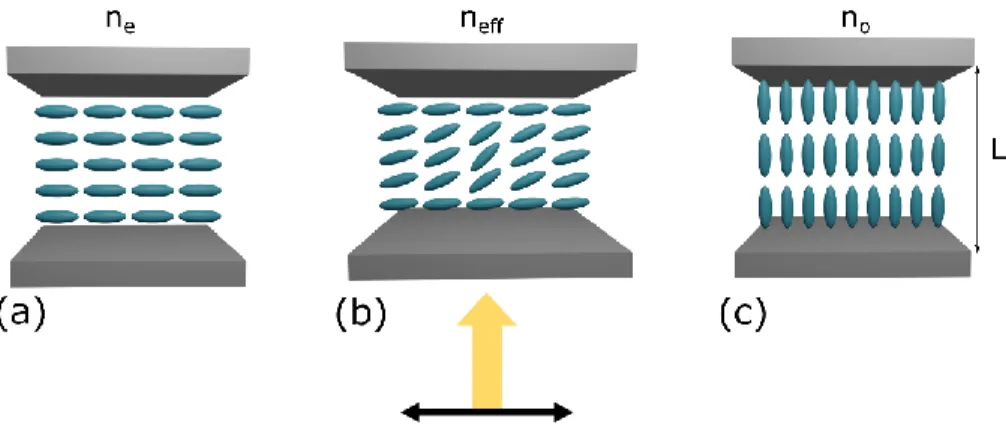
Let us consider a planar LC cell with linearly polarized light normally incident on it. Optical axis is parallel to director. Depending on the orientation of LC molecules the beam experiences different refractive indices. Optical path for the beam passing LC cell of thickness L, as demonstrated in Figure I.7 (a) is neL, when for situation depicted in Figure I.7 (c) it is noL.

Figure I.7. Dependence of refractive index encountered by incident beam on director orientation (black arrow – direction of polarization, yellow arrow – direction of propagation).

When director makes an angle with beam’s polarization direction (Figure I.7 (b)), the effective refractive index is

2 2 2 2

,

o e eff e

co

o

n n

n

s

n si

n



n



=

+

(I.33)

as it was shown in section I.3.

Because ordinary and extraordinary beams face different refractive indices, there will be a phase retardation between them, that can be calculated as

2 (x, ,z) .

eff

n

y

dz







=



(I.34)

It is possible to create such a distribution of effective refractive index that phase profile of extraordinary beam at the exit from the LC cell will be similar to that of a beam passing through an ordinary lens. Numerous techniques providing electric field modulation within LC cell to create

(32)

gradual variation of refractive index exist. Moreover, as molecular orientation is controlled with application of voltage, we can change the shape of final phase profile, varying optical power and aberrations as well.

Many designs of adaptive liquid crystal lenses have been presented in recent years. In the following sections we will briefly discuss the evolution of adaptive LC optics and show several examples of these designs. Then we will introduce the designs that have been investigated during this project and that will be discussed in detail in the subsequent chapters of this thesis.

I.7 Overview of existing tunable liquid crystal lens designs

Tunable lenses have always been of great interest because they have numerous applications not only in scientific domain, but in everyday use devices as well (phone cameras, web cameras, etс.). Today we know various approaches to create a tunable lens, starting from a straightforward mechanical displacement of an ordinary lens, ending with liquid lenses formed within elastomeric membranes. Although some optical systems use these types of lenses, there exists an even more elegant approach of liquid crystal-based tunable lensing. We may notice that existing tunable lenses often mimic eyes of wild birds or animals. For example, some bird species have the ability to deform their eyes [21] to focus on prey or other particular objects of interest. On the other hand, we have liquid lenses that achieve the change of optical power via variation of elastic transparent membrane’s curvature when a liquid is injected or pulled out. Another possibility is to deform a drop of liquid using electrowetting effect [15].

However, the approach of liquid crystal tunable lenses stands out. These lenses have visible advantages: exclusion of mechanical movement, easy control, relatively simple fabrication, low cost and high image quality. A simple LC cell can act as a lens if we shape the electric field in such a way that it creates parabolic distribution of LC director within the cell. This leads to a parabolic distribution of effective refractive index. Thus, a plane linearly polarized wave acquires spherical phase retardation as it passes through the cell. Depending on the distribution of molecules we can equally create lenses with negative or positive optical powers. As the reorientation of molecules varies gradually with the application of voltage – we achieve controllable change of focal distance. The concept of liquid crystal lenses was developed by S. Sato. In one of his first papers dedicated to this subject he described the possibility of making switchable lenses using LCs (Fig. I.8) [22].

(33)

Figure I.8. One of the first LC lens designs [22].

In this case the lens consisted of a flat and a concave glass substrates covered with transparent electrodes (ITO). The gap in between them was filled with LC, which enabled shifting between two focal points as voltage was turned on or off.

Tunable liquid crystal lenses have greatly evolved over the past decades, overcoming many limitations of other types of adaptive lenses (slow response, high aberrations, gravitational effect in case of liquid lenses). This field remains competitive, as new designs of liquid crystal lenses emerge. All LC based lenses can be divided into several categories [23], for example: curved lenses (shown in Fig. I.8), gradient index (GRIN) lenses (Figures I.9 and I.10), composite lenses (combinations of curved and GRIN types), Fresnel lenses (Figure I.11). The difference among designs is defined mainly by the means of shaping the electric field inside the LC cell. Let us take a closer look at several designs representing different categories.

There are many variations of GRIN LC lens designs. This type of lenses usually involves the presence of a supplementary layer, which shapes the electric field. This could be, for example, a layer of dielectric fabricated in such a way that its permittivity decreases quadratically from the center to the periphery. One of the first LC-based GRIN lenses was reported by Sato, Figure I.9 [24].

(34)

In this case the top electrode (made from ITO or aluminum) has a hole pattern of predefined diameter. Inner surfaces of the cell are covered with polyimide (not shown in Fig. I.9). The polyamide layers were rubbed in anti-parallel directions to ensure homogenous alignment of molecules. An intermediate upper glass substrate (located right below hole patterned electrode) ensures gradual drop of electric field potential, which decreases from the edge of the aperture towards the center. This, in turn, creates parabolic distribution of director’s orientation. However, in the absence of additional glass layer, we would observe an abrupt change in electric potential close to the edge of circular electrode and the lens would not function properly, as the formation of disclination lines (defects) would be highly probable. The advantages of this design are the simplicity of photolithography and the possibility of creating LC lenses of relatively large aperture sizes (the lens of 7 mm diameter was characterized by Sato). However, the operating voltages for this design remain rather high [25] due to the glass layer that softens electric field.

One of the simplest ways to create a parabolic electric potential distribution is to use a curved electrode. Such a design, demonstrated in Figure I.10 was published by Wang et al [26]:

Figure I.10. Schematics of an LC lens with a curved electrode [26].

The lens consists of a standard LC cell with initial planar alignment and a plano-convex glass lens in contact with one of the cell’s substrates. The convex surface of the glass is covered with a thin transparent conductive ITO film. The opposite inner side of the cell is coated with ITO as well. Polyamide layers deposited on the inner walls of the cell were mechanically treated to provide initial orientation of director. When voltage is applied to the electrodes, we observe more director reorientation at the periphery of the glass lens (as we have higher values of electric potential in these areas due to proximity of top electrode). Director’s reorientation gradually decreases from the periphery towards the center of the cell at fixed applied voltage. Resulting device acts as a tunable lens. It is worth noticing that even when no voltage is applied, this system will still be focusing light, as its total optical power is the sum of optical power coming from a glass lens and variable optical

(35)

power from LC cell. Initial focal distance (at V=0) is defined only by contribution from the plano-convex lens. When voltage is increased – LC starts reorienting, increasing total optical power. As voltage is increased further, director becomes reoriented not only at the edge of the aperture but in the center as well, thus decreasing optical power coming from LC cell. One of the main drawbacks of this design is residual optical power in ground state. Also, relatively high voltages are required for operation.

A common problem faced by LC lenses is their inability to achieve high optical powers for a wide aperture (> 4 mm) and maintain other characteristics simultaneously (low scattering levels, low aberrations, fast reorientation). One possibility to increase the optical power is to make thicker LC cells, because it is directly proportional to cell’s height. But this solution comes with some tradeoffs, such as larger excitation times and increasing scattering. However, certain designs enable us to obtain higher optical powers, preserving normal excitation times and image contrast.

A concept proposed by the group of Bos [27] adapts a well-known approach of refractive Fresnel lens (Figure I.11).

Figure I.11. Scheme of refractive Fresnel lens described in [27].

First, a glass substrate is covered with concentric ITO rings of equal areas separated by gaps using photolithography. Every pair of neighboring ring electrodes is connected with a resistor that serves to decrease electric potential, propagating from one electrode to the other. The first layer of patterned ITO is then covered with dielectric (SiO2) in which openings are made to connect to external bus lines by means of nickel deposition and patterning. In total, the first substrate has 288 ring electrodes, several of them are directly connected to bus line electrodes (see Ni in Figure I.11). Then a new layer of dielectric is deposited, insulating the first layer of ITO and bus line connections. Finally, the second layer of ITO is deposited and patterned to form concentric rings that are slightly shifted relative to the first layer. Inner surface of the second substrate is covered with one layer of

(36)

ITO that serves as common ground. Both substrates are then covered with polyamide, rubbed in antiparallel directions, and glued together.

Application of voltage to bus line connections creates an abrupt reorientation of LC director in certain parts of the lens, where ring electrodes are connected directly. Electric potential drops on interelectrode resistors until another electrode with direct connection appears, causing another jump of potential. In such a way it is possible to obtain the phase pattern with several phase resets, resembling the one of a conventional Fresnel lens, where similar phase profile is achieved by means of relief structures.

Creating phase resets the authors managed to obtain desired optical power and maintain fast reorientation of the lens, but the fabrication process is complex and involves several steps of photolithography and deposition. Resulting device is a switchable Fresnel lens.

Although a great number of LC lens designs have been reported, they all possess some limitations. It is often required to have a large diameter lens, but the maximal achievable optical power of an LC lens decreases quadratically with the increase of clear aperture’s radius. In order to have a wide dynamic range of optical powers we need a big difference of phase retardation between central and peripheral portions of the lens. It can be obtained if we increase the cell’s thickness, but then the response times will increase as well. Another problem that comes with making thicker LC cells is scattering, which degrades contrast and resolution. The important aspect for mobile applications is power consumption. Therefore, designs that require high voltages might be inappropriate.

It is preferable to have a simple experimental procedure for lens assembly, because every additional step increases unit price. LC lenses are polarization dependent, unless the final device is composed of two lenses with one having rubbing direction turned 90 degrees relative to the other. Finally, the aberrations should be minimized to provide the best image quality.

It is rather challenging (almost impossible) to create a design that would overcome all the above-mentioned limitations. On the other hand, we can find good application targeted solutions. In the next section we will describe the lenses that have been broadly studied in this thesis. They proved to have some advantages in comparison with existing concepts, which will be further discussed in detail.

Theoretical and experimental study of tunable liquid crystal lenses : wavefront optimization