O
pen
A
rchive
T
OULOUSE
A
rchive
O
uverte (
OATAO
)
OATAO is an open access repository that collects the work of Toulouse researchers and
makes it freely available over the web where possible.
This is an author-deposited version published in :
http://oatao.univ-toulouse.fr/
Eprints ID : 15336
The contribution was presented at PAAMS 2015 :
http://www.paams.net/
To cite this version :
Cazin, Nicolas and Histace, Aymeric and Picard, David and
Gaudou, Benoit On The Joint Modeling of The Behavior of Social Insects and Their
Interaction With Environment by Taking Into Account Physical Phenomena Like
Anisotropic Diffusion. (2015) In: 13th International Conference on Practical
Applications of Agents and Multi-Agent Systems (PAAMS 2015), 3 June 2015 - 4
June 2015 (Salamanca, Spain).
Any correspondence concerning this service should be sent to the repository
administrator:
[email protected]
On The Joint Modeling of The Behavior of Social Insects and Their
Interaction With Environment by Taking Into Account Physical
Phenomena Like Anisotropic Diffusion
Nicolas Cazin1, Aymeric Histace1, David Picard1, and Benoît Gaudou21ETIS, ENSEA, University of Cergy-Pontoise, CNRS, Cergy-Pontoise, France 2IRIT, University of Toulouse, Toulouse, France
[email protected], [email protected], [email protected], [email protected]
Abstract This work takes place in the framework of GEODIFF project (funded by CNRS) and deals with the general issue of the social behavior modeling of pest insects with a particular focus on Bark Beetles. Bark Beetles are responsible for pine trees devastation in North America since 2005. In order to stem the problem and to apply an adapted strategy, one should be able to predict the evolution of the population of Bark Beetles. More precisely, a model taking into account a given population of insects (a colony) interacting with its environment, the forest ecosystem, would be very helpful. In a previous work, we aimed to model diffusive phenomenons across the environment using a simple reactive Multi-agent System. Bark beetle use pheromones as a support for recruitment of other bark beetles in the neighborhood in order to achieve a mass attack over a tree. They are first attracted by the ethanol or other phytopheromones emitted by a sick, stressed or dead tree and reinforce the presence of other individuals amongst the targeted tree. Both ethanol and semiochemicals are transported through the forest thanks to the wind, thermic effects and this advection phenomenon is modulated by the topology of the environment, tree and other obstacles distribution. In other words, the environment is involved in the process of a bark beetle attack. The first modeling we used to tackle our objective was not spatially explicit as long as free space propagation only was taken into account (isotropic phenomenon) with no constraint imposed by the environment such as wind. This article is intended to take into account such physical phenomenons and push the modeling one step further by providing predictions driven by measures provided by a Geographical Information System.
1
Introduction
Modeling of the population dynamics is an essential part of both research and management of forest pest insects. These kind of complex objectives require prediction of population changes over long time intervals and over large areas. Of course, it is impossible to predict pest abundance at specific location ten years ahead, but it may be possible to predict the change in average pest population density as a result of some change in environment.
Formerly, to tackle this objective, mathematical modeling was the major tool for predicting population dynamics and the reader could refer to Berryman and Millstein [1] for a complete overview of some of the most known models that are mainly based on modifications of discrete-time analog of the logistic model. The main advantage of such methods is that parameters of these models can be adjusted to fit available data. Nowadays, mathematical modeling based approaches tend to be replaced by Multi-agent Modeling (MAM) based ones that has constituted an important research and development area for the past two decades [2].
Aim of this article is to propose a MAM based on a simple reactive Multi-agent System (MAS) [3,4] with possibility to take into account evolution physical laws related to the corresponding environment. More pre-cisely, we want to show that by integrating the way the resources and the trail markers could naturally vanish, steered by a diffusive phenomenon parametrically described using a spatio-temporal like heat equation, we can obtain a more realistic modeling of the global behavior of the MAS dynamics.
Practically speaking, we focus our attention on the behavior modeling of a particular social pest insect: the “Bark beetle". Bark beetles or “Scolytes” are ecologically and economically significant [5] since outbreak species help to renew the forest by killing older trees and other species aid in the decomposition of dead wood. However, several outbreak-prone species are known as notorious pests that can cause tremendous damage to pine tree forests for instance [6]. As a consequence, a better understanding of the social behavior of this beetle would definitely be of some precious help to limit its damage capability.
This article is organized as follows: In Section 2, the model used for experiments is presented and de-tailed. In Section 3, different scenarios are considered for experiments in order to show that the proposed modeling is realistic and can adapt to non-classic situations including anisotropic phenomenons like wind. In the last section, conclusion and discussion are proposed.
2
Materials and Modeling
2.1 GAMA platform
In the context of this work, the GAMA platform was used [7,8,9]. GAMA is a freely available modeling and simulation development environment for building spatially explicit agent-based simulations. GAMA platform allows to:
– Design, prototype and write models in the GAML agent-oriented language and its optional graphical modeling tool.
– Instantiate agents from any kind of dataset, including GIS data, and execute large-scale simulations (up to millions of agents).
– Couple discrete or continuous topological layers, multiple levels of agency and multiple paradigms (mathematical equations, control architectures, finite state machines).
– Define rich experiments on models and explore their parameters space for calibration and validation. – Design rich user interfaces that support deep inspections on agents, user-controlled actions and panels,
multi-layer 2D/3D displays and multiple agent aspects.
Because of the related flexibility and the possibility to enrich the existing functions in GAML language, the GAMA platform appears as the best solution, providing us the tools to create our complete environment, including complex phenomena as anisotropic ones (winds for instance).
2.2 Static Model
The static model considered in this work was introduced in [10]. Synthetically, the concentration of chemical agents in the environment is modeled according to a Gaussian law decreasing as and when the distance to the tree is increasing. The scolytes and trees behavior is controlled by a finite state automaton owned by each agent. This way, specific operation are realized by each agent, in accordance with a specific internal state at a given instant. The model is constituted of three species (Scolyte, Tree, Environment cell) and their description are mutually dependent. There is no optimal order for describing each one. In the following, each aspect of the model (environments, agents, interactions and related physical laws) are detailed.
Environment The environment is discretized in a finite number of square cells noted(x, y). Each cell is characterized by two variables modeling (i) the amounts of ethanol and (ii) the quantity of pheromones in the cell.
Ethanol The amount of ethanol available in cell(x, y) at time t is given by : E(x, y, t) =X
s∈S
Es(t)e−γ[(x−xs)
2+(y−ys)2]
(1)
withS being the set of trees in ALIVE state, Es(t) being the amount of ethanol emitted by the s tree (of
spatial coordinate(xs, ys)), at time t, given by equation (5).
Pheromones The amount of aggregation pheromones available in a(x, y) cell at time t is given by : P h(x, y, t) =X
s∈S
P hs(t)e−γ[(x−xs)
2+(y−ys)2]
(2)
withS being the set of trees in ALIVE state, P hs(t) being the amount of aggregation pheromones emitted
by the scolyte located in cell(x, y) given by the equation (7).
Attractiveness The attractiveness of a cell(x, y) is defined as a convex combination of the amounts of contained chemical agents given by :
A(x, y, t) = ηP h(x, y, t) + (1 − η)E(x, y, t) (3) withη being the coupling coefficient chosen empirically between 0 and 1.
Tree A tree lying in a(xs, ys) cell is noted s(x, y). This tree represents an amount of resource for scolytes
notedRs(t) and this variable is evolving according to the number of scolytes present in the s(x, y) cell. For
all experiments, we use the usual logistic law of Eq. (4) to model the evolution of the resources on a site.
Rs(t + 1) = Rs(t) − αns(t) (4)
– α being a constant representing the average consumption rate of the resource by a scolyte between two infinitesimal time steps.
(4) is a positive or null amount. The behavior of a tree is described by two states :
ALIVE The tree is alive. This is the initial state of each tree. All along its lifespan, it will rot and emit in the environment an amount of ethanol notedEs, proportional to a fractionµ of the remaining ressources
Rs. The ethanol amount emitted by a trees(x, y) at time t is given by :
Es(t) = µRs(t) (5)
A tree will switch to the DEAD state whenRs(t) = 0.
Scolyte A scolyte contained in a given cell(x, y) is noted a(x, y). The behavior of a Scolyte [11,12,13] is described by three main states :
INIT This is the initial state of a scolyte after its instantiation. This is a technical state added in order to work around a constraint of the GAML language stating that an initial state must be declared. More than anything, the initial state of a scolyte agent may be different according to its initial location or experi-ment constraints. It is impossible to force the initial state during the instantiation. A transition towards the FLYING state is trigged if the scolyte is in a cell containing an ALIVE tree. Otherwise, a transition towards the EATING state is trigged.
FLYING In this state, the scolyte will choose the next cell he will visit by using its local perceptions. The immediate neighborhood of the cell occupied by thea agent is noted N (a). The scolyte will fly towards the cell(x⋆, y⋆) from the N (a) cell with a probability related to the cell attractiveness. The probability for a scolyte to move in the cell(x⋆, y⋆) is given by :
pa(t)(x⋆, y⋆) =
A(x⋆, y⋆, t) P
(x,y)∈N (a)A(x, y, t)
(6) withA(x⋆, y⋆, t) the attractiveness of the (x⋆, y⋆) cell, at instant t. Then, the target cell is determined thanks to a barrel roll algorithm, i.e. by scanning the attractivity of each possible in a 8-connectivity neighborhood. Several copies of each cell are inserted in a list. The number of copies of each cell is proportional to the associated transition probability towards this cell. If no cell is really attractive, all transitions are with same probability and the cell is thus randomly selected inN (a). This probabilistic roaming gives the opportunity to each agent to move sometimes in a cell different than the most attrac-tive cell. Since the new surrounding cells may be close to another potential well, the scolytes are allowed to separate from the colony and explore new areas of the environment.
EATING When the scolyte lands in the cells(x, y) containing a tree, it consumes the Rsresource by eating
aµ fraction and emitting a v amount of aggregation pheromones in the s(x, y) cell. This cell becomes more attractive for the other scolytes. The amount of pheromones emitted by the scolytes in thes(x, y) cell at timet is given by :
P hs(t) = ν ∗ ns(t) (7)
withν the amount of aggregation pheromones emitted by a single scolyte.
At each iteration, the departure probability of the scolytea to move from the s source is given by : qa(t) = 1 − R
s(t)
Rs(0)
(8) The transition towards the FLYING state is related to the probabilityqa(t). A variable between 0 and 1
is randomly selected in a uniform distribution. If the result is less than (8), the transition to the FLYING state occurs. Otherwise, the scolyte stays in the EATING state.
2.3 Diffusion/Reaction
Formerly introduced in [14] for MAS Modeling, matter diffusion is an irreversible transport phenomenon and one may define it by the trend of a system to converge towards a homogenous concentration of chemical agents. The diffusion equation is given by :
∂φ(r, t)
withr the cell where the φ density, sampled at time t, is set, D(φ, r) is the diffusion coefficient for the φ density sampled at placer, and D(φ, r) may be an input from a GIS.
By considering the diffusion coefficient as a constant value over the wholeR map1, the equation (9)
may be rewritten as :
∂φ(r, t)
∂t = DΦ· ∇
2· φ(r, t) (10)
This is the well known heat equation. By consideringr = (x, y), first order spatial derivatives along X and Y axis, the square cell hypothesis and the 8-connexity of the cells, Eq. 10 may be solved on the discrete time case by :
ΦR(t + 1) = ΦR(t) ∗ GD (11)
withΦR(t) = (φ(x, y, t))x∈Rx,y∈Ry being the concentration of a given chemical reagent in theR space
(square in this case),GD = DΦ16 ·
1 2 1 2 16 DΦ − 12 2 1 2 1
being a stencil describing the neighborhood influence in the diffusive phenomenon related to the constant diffusion coefficientDΦ.
If the diffusion coefficient is a constant, then the diffusion equation is a simple convolution with a3 × 3 mask. This mask is Gaussian forDΦ= 1. Knowing that trees emit ethanol while decaying and that scolytes
emit pheromones during an attack to attract other agent of the same species, on may consider emission as a chemical diffusive phenomenon. Letqφ(x, y, t) be the amount of chemical reagent φ at cell (x, y) and time
t. qφ(x, y, t)
> 0 when the chemical reaction is active. = 0 when there is no chemical reaction.
< 0 when the chemical reaction is destroying reagents. The equation (11) is now extended by :
ΦR(t + 1) = ΦR(t) ∗ GD+ QΦR(t) (12)
withQΦR(t) being the amount of created (or vanished) chemical reagent φ by the chemical reactions
hap-penings over the wholeR map (It is also called the the reaction term), and ΦR(t) ∗ GDis the diffusion term.
It is a solution to the diffusion reaction equation.
2.4 Diffusion/Reaction/Evaporation
The current update equation (12) is still not so realistic. Suspended chemical agents may have a limited persistence. This persistence depends mainly on moisture and ambient temperature. Without a deep un-derstanding of complex chemical reaction, we propose to simply model the evaporation as a progressive reduction of the current amount of chemical agent. The amount mapQΦR(t) is simply extended as :
QEv
ΦR(t) = QΦR(t) − EvΦ· ΦR(t) ∗ GD (13)
withEvΦbeing the evaporation constant between0 and 1. It represents the amount of diffused ΦR(t) being
evaporated, andQΦR(t) is the simple reaction term.
1D(φ, r) = D
A fractionEvΦof the diffused amountΦR(t) ∗ GD is subtracted from the current amount for chemical
reagentsQΦR(t). By plugging this extended reaction term (13) in equation (12), it comes :
ΦR(t + 1) = (1 − EvΦ) · ΦR(t) ∗ GD+ QΦR(t) (14)
Only a fraction1 − EvΦof the diffusion term is kept. LikeDΦ,EvΦis chosen constant over the wholeR
map for simplicity purpose but it may be kept variable, for instance by taking into account measures from a GIS
2.5 Diffusion/Reaction/Evaporation/Advection
The wind phenomenon may be modeled by the advection equation. The advection of a scalar quantity may be written as the gradient of the average velocity vector moving aΦ amount of chemical agent. By using the finite elements method and first order spatial derivatives, the equation (14) becomes :
ΦR(t + 1) = (1 − EvΦ) · (ΦR(t) ∗ GD− v · Φ(x, y, t) ∗ 0 0 0 −1 0 1 0 0 0 Φ(x, y, t) ∗ 0 −1 0 0 0 0 0 1 0 ) + QΦR(t) = (1 − EvΦ) · (ΦR(t) ∗ GD− ΦR(t) ∗ 0 −vx 2 0 −vx 2 0 vx 2 0 vy2 0 ) + QΦR(t) = (1 − EvΦ) · (ΦR(t) ∗ GD− ΦR(t) ∗ V ) + QΦR(t) = ΦR(t) ∗ (GD− V ) · (1 − EvΦ) + QΦR(t) (15)
The advection is represented by a stencilV opposed to the diffusion stencil GD. This scheme is unstable
forkvk > 1. The initial model (11) is based on a forward Euler method with a unitary time-step2. One
can rewrite the model using the Euler forward method or a higher order method (like the Runge-Kutta 4) in order to avoid numerical instability problems. In [15], the author proposes a method based on the reverse scheme. By considering the displacement vector as the variation of ther(t) position of a particle during a short time-lapse, one may write :
r(t + 1) − r(t)
∆t = u(t) (16)
Ther(t + 1) may be deduced from r(t) and u(t)
r(t + 1) = r(t) + ∆t · u(t) (17)
Instead of moving an amount of chemical reagent from one point to another, the placer where the advected amount is originated will be determined by inverting the advection vector direction.
q(r, t + 1) = q(r − u(r, t) · ∆t, t) (18) The pointrsource = r − u(r, t) · ∆t is not a exactly a discrete cell coordinate but a point located between
the 4 adjacent cells of the source. The amountq advected from rsource is determined thanks to a bilinear
2φ(r, t + h) = φ(r, t) + h∂φ(r,t)
interpolation between the amounts contained in the 4 adjacent cells of the source. This interpolated amount is added tordestinationand subtracted from the 4 adjacent cells of the source, proportionally to their
contri-bution weighting in the bilinear interpolation. The advected amounts are conserved ([16]). The velocity map may be precomputed in order to take into account several obstacles such as trees in the environment.
3
Experiments and Results
The following experiments aim to exhibit the effect of wind on the colony’s next move. Wind is advecting semiochemicals and ethanol. The attractiveness of an area from the point of view of the Scolyte is driven by the concentration of semiochemicals and ethanol. From a upper point of view, It may be interpreted by a concentration map of reagents on the forest ecosystem. Any modulation of the "density map" could lead to a different behavior of a colony and may have several consequences on the other actors of the ecosystem due to their tight coupling.
3.1 Double-Well Potential Function
This is the reference experiment. The colony converges towards the nearest tree, consumes all its resources and then forages for the next host tree. This is the straight implementation of the model introduced in Section (2). The only source of non determinism in this simulation is the stochastic probabilistic selection of the next cell, a random “walk" algorithm.
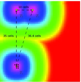
Description The grid world is set up with a50 × 50 empty array of semiochemicals and ethanol. Scolytes are initially consuming the first tree at coordinates(20, 5) and each of the three provide the same amount of ressource (arbitrarly set to 1000). The figure 1 displays this configuration. The attraction map is colored according a logarithmic scale described by the following equation :
((h, s, v), x, y) = (((grid[x][y] − M IN )/(M AX − M IN ), 1.0, 1.0), x, y) (19) With :
– grid[x][y] = 10 · log10(attractiveness[x][y])
– M IN = −300dB
– M AX = 10 · log10(1000)dB
The red color denotes a non attractive cell3and a pink cell denotes a very attractive cell4
3attractiveness[x][y] = M IN 4attractiveness[x][y] = M AX
Tl Tr
Ti
Figure 1: Attractiveness map state at initial configuration. The initial tree is namedTrand have(20, 5) grid
coordinates, the leftmost tree is namedTland have(10, 5) grid coordinates, the rightmost tree is named Ti
and have(10, 40) grid coordinates.
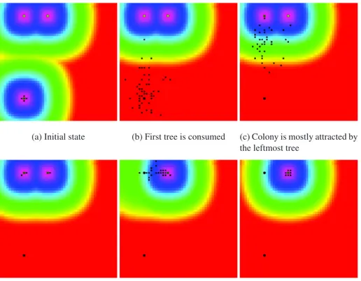
Observations Figure 2 depicts the colony’s path through the forest.
1. The colony is initially set on theTitree (Figure 2a). The surrounding cells are less attractive than the
immediate neighborhood ofTi. The all colony is aggregated on this particular location of the map.
2. Scolytes are consumingTiresources and will move towards the closest treeTlonce totally consumed
(Figure 2b). The tree stop emits ethanol and scolytes stops emit pheromones. After evaporation of the remaining amounts of reagents, the attractiveness gradient is now positive and scolyte will be trapped by the closest potential well.
3. According to the scolytes perception, the most interesting bearing is given by the closest tree. Almost the entire colony is consuming theTltree (Figure 2c). Due to the randomized/probabilistic move of
each agent, a small part of the population is sometimes set at a random location according to a given probability.
4. Colony is mostly located on theTltree (Figure 2d) and the remaining agents are consuming theTrtree.
5. Once Tl is left dead, the colony converges quickly towards the remaining Tr tree (Figure 2e). The
attractiveness around Tl decreases since all over no more ethanol nor pheromones are emitted. The
remaining chemical products are evaporated. The gradient becomes positive and the colony is no longer trapped aroundTl
6. The whole colony is consuming theTrtree resources(Figure 2f). They are trapped but the potential well
induced by ethanol and pheromones emission.
Each agent is following the shortest path to the local maximum of attractiveness when not wandering. The random exploratory strategy is useful for handling the case where attractiveness gradient is not relevant. The path of the colony in this experiment is summarized by(Ti→ Tl→ Tr)
(a) Initial state (b) First tree is consumed (c) Colony is mostly attracted by the leftmost tree
(d) Colony is consuming left-most tree
(e) Colony is moving towards rightmost tree
(f) Colony is consuming the last tree
Figure 2: False color attractiveness map, No wind experiment
3.2 Wind Influence
This experience aims to demonstrate the effect of the wind on the colony’s trend in choosing the most attractive cells when flying.
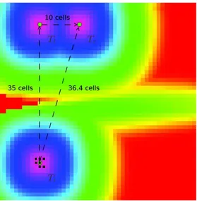
Description The same configuration as in the previous experiment is kept and is extended by adding a wind corridor. The figure 3 displays the effect of wind on the attractiveness map. Clearly, amounts of ethanol and pheromones are transported from one cell to another.
Tl Tr
Ti
Figure 3: Attractiveness map state at initial configuration with a wind corridor. The initial tree is named Tr and have(20, 5) grid coordinates, the leftmost tree is named Tland have(10, 5) grid coordinates, the
rightmost tree is namedTiand have(10, 40) grid coordinates, the wind corridor is 10 cells wide and directed
along thex axis.
Observations Figure 4 depicts the colony’s path through the forest modified by the advection of semio-chemicals.
1. The colony is initially set on theTitree (Figure 4a). The surrounding cells are less attractive than the
immediate neighborhood ofTi. The colony is focused those cells.
2. Scolytes are consumingTiresources and will move towards the most interesting cells once totally
con-sumed (Figure 4b). The attractiveness gradient is now positive and scolyte will be trapped by the closest potential well.
3. According to the scolytes perception, the most interesting bearing is now towards theTr tree which
is not the closest tree. Almost the entire colony is consuming theTr tree (Figure 4c). Due to the
ran-domized/probabilistic move of each agent, a small part of the population is sometimes set at a random location according to a given probability.
4. Colony is mostly located on theTrtree (Figure 4d) and the remaining agents are consuming theTltree.
5. OnceTrleft dead, colony converges quickly towards the remainingTltree (Figure 4e). The
attractive-ness aroundTlis lowered since over the no more ethanol nor pheromones are emitted. The remaining
chemical products are evaporated. The gradient becomes positive and the colony is no longer trapped aroundTr
6. The whole colony is consuming theTltree resources (Figure 4f). They are trapped but the potential well
induced by ethanol and pheromones emission.
(a) Attractiveness at t= 43 (b) Attractiveness at t= 188 (c) Attractiveness at t= 228
(d) Attractiveness at t= 236 (e) Attractiveness at t= 249 (f) Attractiveness at t= 263 Figure 4: False color attractiveness map with a wind corridor
4
Discussion, Conclusion, Perspectives
In this article, a MAS approach is proposed for modeling of the behavior of pest insects, not only consid-ering their classic social interactions using hormones, but also by the taking into of the external physical phenomena that characterized the environment in which the agents are living (linear and non -linear diffu-sion). This work extends former work of Langlois et al [14] in which only simple linear phenomenon were taken into account in chemical agents diffusion process modeling and is new considering applications to the modeling of ant-like insects’ behavior. The 3.2 section shows that modeling physical phenomenon by taking into account measurements extracted from a GIS allows the hybrid MAS-PDE simulator GAMA to provide more realistic forecasts. In other words, the agent’s behavior is modified thanks to their interaction with the environment and their peer trough the environment. This environment is no longer static and have its own dynamic, like the other agents. Each cell from the grid world and each particle of chemical reagent may be considered as a particular agent. We use simplified fluid dynamics usual equations in order to demonstrate the feasibility of a joint MAS-PDE modeling tool. This work is easily extendable to GP-GPU fluid dynamics and MPI clustering in order to support larger scale problems. From a modeling point of view now, the current model have several limitations :
– The advection model is incomplete and have no support for viscosity. The amounts of chemical reagents are like teleported from one point or another without any resistance to advection. The velocity map needs to be updated at each step according by the perturbations resulting from the viscosity forces modeling.
– pressure, topology, heat, moisture have a major influence on the velocity map and need
– Real world is in three dimensions and our grid world have only two dimensions. Temperature differences play an important role in the determination of the velocity map
– The size of the environment, agents and their parameters, different timescales have to be studied and fixed
– The behavior of scolytes is incomplete: Eggs, larvaes, females, males scolytes have different behaviors and different needs. Other pheromones play an important role in local competition handling and colonies formation.
– Dynamic environments also have an influence on scolytes, such as wind carrying the agents.
– Other actors/phenomenons of the ecosystem need to be modeled. Especially, human and forest manage-ment, fires, water and temperature.
To overcome these limitations, tools inspired coming from large scale fluid dynamics simulations could be of real interest and integrating these real-time computing methods in the MAS-PDE simulator could permit to have a modeling of the insects’ behavior always more realistic, which is of primary importance for an efficient and anticipated management of the pest insect populations.
References
1. Berryman, A.A., Millstein, J.A.: Population analysis system. Pullman edn., Washington (1994) Version 4.0. 2. Ferber, J.: Multi-Agent Systems: An Introduction to Distributed Artificial Intelligence. Addison-Wesley (1999) 3. Drogoul, A.: Résolution Collective de Problèmes : Une étude de l’émergence de structures d’organisations dans les
systèmes multi-agents. PhD thesis, Université Paris VI (1993)
4. Rouchier, J. In: Systèmes multi-agents et modélisation de systèmes sociaux. Hermes science (2002) 285–299 5. Bentz, B.: Climate Change and Bark Beetles of the Western United States and Canada: Direct and Indirect Effects.
BioScience 8(60) (2010) 602–613 doi:10.1525/bio.2010.60.8.6.
6. Robins, J.: Bark Beetles Kill Millions of Acres of Trees in West. New York Times, 17 November (November 2008) 7. Amouroux, E., Chu, T.Q., Boucher, A., Drogoul, A.: Gama: an environment for implementing and running spatially explicit multi-agent simulations. In: Principles and Practice of Multi-Agent Systems. Volume 5044., Springer (2009) 359–371
8. Taillandier, P., Vo, D.A., Amouroux, E., Drogoul, A.: Gama: a simulation platform that integrates geographical information data, agent-based modeling and multi-scale control. In: Principles and Practice of Multi-Agent Systems. Volume 7057., Springer (2012) 242–258
9. Drogoul, A., Amouroux, E., Caillou, P., Gaudou, B., Arnaud, G., Marilleau, N., Taillander, P., Vavasseur, M., Duc-An, V., Jean-Daniel, Z.: Gama: Multi-level and complex environment for agent-based models and simulations. In: Proceedings of the 2013 international conference on Autonomous agents and multi-agent systems. (2013) 1361– 1362
10. Picard, D., Histace, A., Desseroit, M.C.: Joint mas-pde modeling of forest pest insect dynamics : Analysis of the bark beetle’s behavior (2013)
11. Byers, J.A.: Behavioral mechanisms involved in reducing competition in bark beetles. HOLARCTIC ECOLOGY 12 (1989) 466–476
12. Bakke, A.: Using pheromones in the management of bark beetle outbreaks. In: Patterns of Interaction with Host Trees. (1991) 371–377
13. Harrington, T.C.: Ecology and evolution of mycophagous bark beetles and their fungal partners. In Press, O.U., ed.: Ecological and Evolutionary Advances in Insect-Fungal Associations, Vega, F. E. and Blackwell, M. (2005) 257–291
14. Langlois, P., Daudé, E.: Concepts et modélisation de la diffusion géographique. cybergeo. In: European Journal of Geography, http://www.cybergeo.eu/index2898.html (2007)
15. Stam, J.: Real-time fluid dynamics for games. In: Proceedings of the Game Developer Conference. (2003) 16. West, M.: Practical fluid dynamics: Part 1. Game Developer magazine (2008)