Forecasting variations and trends in water main breaks

Publisher’s version / Version de l'éditeur:

Journal of Infrastructure Systems, 8, December 4, pp. 122-131, 2002-12-01

READ THESE TERMS AND CONDITIONS CAREFULLY BEFORE USING THIS WEBSITE.

https://nrc-publications.canada.ca/eng/copyright

Vous avez des questions? Nous pouvons vous aider. Pour communiquer directement avec un auteur, consultez la première page de la revue dans laquelle son article a été publié afin de trouver ses coordonnées. Si vous n’arrivez pas à les repérer, communiquez avec nous à PublicationsArchive-ArchivesPublications@nrc-cnrc.gc.ca.

Questions? Contact the NRC Publications Archive team at

PublicationsArchive-ArchivesPublications@nrc-cnrc.gc.ca. If you wish to email the authors directly, please see the first page of the publication for their contact information.

NRC Publications Archive

Archives des publications du CNRC

This publication could be one of several versions: author’s original, accepted manuscript or the publisher’s version. / La version de cette publication peut être l’une des suivantes : la version prépublication de l’auteur, la version acceptée du manuscrit ou la version de l’éditeur.

For the publisher’s version, please access the DOI link below./ Pour consulter la version de l’éditeur, utilisez le lien DOI ci-dessous.

https://doi.org/10.1061/(ASCE)1076-0342(2002)8:4(122)

Access and use of this website and the material on it are subject to the Terms and Conditions set forth at

Forecasting variations and trends in water main breaks Kleiner, Y.; Rajani, B. B.

https://publications-cnrc.canada.ca/fra/droits

L’accès à ce site Web et l’utilisation de son contenu sont assujettis aux conditions présentées dans le site LISEZ CES CONDITIONS ATTENTIVEMENT AVANT D’UTILISER CE SITE WEB.

NRC Publications Record / Notice d'Archives des publications de CNRC:

https://nrc-publications.canada.ca/eng/view/object/?id=5f2ece78-78a7-4f3c-9ebd-8d780848e387 https://publications-cnrc.canada.ca/fra/voir/objet/?id=5f2ece78-78a7-4f3c-9ebd-8d780848e387

Forecasting variations and trends in water-main breaks

Kleiner, Y.; Rajani, B.

A version of this document is published in / Une version de ce document se trouve dans : Journal of Infrastructure Systems, v. 8, no. 4, Dec. 2002, pp. 122-131

www.nrc.ca/irc/ircpubs NRCC-44677

Forecasting Variations and Trends in Water Main Breaks

Y. Kleiner Member ASCE, and Balvant Rajani Member ASCE

Abstract: The effective planning for the renewal of water distribution systems requires accurate quantification of the structural deterioration of water mains. Direct inspection of all water mains in a distribution system is almost always prohibitively expensive. Identifying water main breakage patterns over time is an effective and inexpensive alternative to gauge the structural deterioration of a water distribution system.

While the structural deterioration of the pipe is generally considered to be a steady, monotone process, some of the environmental and operational stresses acting upon it are time-dependent, steady or transient. These stresses result in sets of “noisy” breakage rate data that often mask the underlying deterioration (ageing) patterns, especially in small data sets. If the cause of these random stresses can be identified and attributed to measurable phenomena (e.g., temperatures, precipitation, etc.), a more accurate pipe deterioration pattern can be obtained. Further, better predictions of water main breakage could be made if these phenomena could be forecast with any degree of accuracy.

A method is presented to analyse how breakage rate patterns of water mains are affected by time-dependent factors. The method is versatile enough to consider any number of underlying factors but the solution becomes more complex, and more data are required as the number of factors increases. A case study is presented to demonstrate the method. Several time-dependent factors were examined, some of which were found to be significant contributors to the time-variation of breakage rates.

Key words: water main deterioration, pipe failure, statistical analysis of water main breaks, time-dependent factors, Fourier analysis, short-term forecast of climate.

Introduction

Distribution networks often account for up to 80% of total expenditures involved in water supply systems. As water mains deteriorate both structurally and functionally, their breakage rates increase, network hydraulic capacity decreases, and the water quality in the distribution system may decline. Scarce capital resources make it essential for planners and decision-makers to seek the most cost-effective rehabilitation and renewal strategies. The ideal strategy should

exploit the full extent of the useful life of the individual pipe, while addressing issues of safety, reliability, water quality, and economic efficiency.

Effective planning for the renewal of water distribution systems requires accurate quantification of the structural deterioration of water mains. Direct inspection of all water mains in a distribution network is often prohibitively laborious and expensive. The application of physical models to assess the structural resiliency of each individual pipe is also not realistic in most cases because accurate data are rarely available and are very costly to obtain. Using statistical methods to identify breakage patterns over time is an effective and inexpensive alternative to measure the structural deterioration of water mains.

The breakage rate of water mains is determined by their deterioration, which is generally a steady monotone process, by environmental conditions (e.g., temperature, precipitation) that are random and often cyclical over time, and by operational factors (e.g., replacement rate, cathodic protection), which may vary over time. The time-varying effects lead to “noisy” annual breakage rates that often mask the underlying deterioration (ageing) patterns, especially in small data sets.

A water utility is typically required to do two levels of planning, short-term for operational purposes and long-term for capital expenditure plans. Short-term planning requires forecasts of the number of water main breaks that are likely to occur in each of the next 3 to 4 years, to ensure that adequate resources (man power and equipment) are readily available to meet anticipated needs. Long-term planning requires accurate quantification of the underlying water mains ageing rates in order to identify the time at which it is more economical to replace rather than to continue repairing the pipe.

This paper outlines an approach that addresses both levels of planning. A multi-variate time-exponential model (Kleiner and Rajani 2000) is used to distinguish between effects of ageing, climate and operations on the breakage rate patterns of water mains. This distinction helps to unmask the “true” underlying ageing of water mains, and subsequently to refine the long-term planning process. A method of using Fourier analysis of historical climate patterns is described, to forecast climate in the next 3 to 4 years (short-term). This method is provided as a rudimentary alternative in cases where more elaborate climate forecasts are unavailable. Forecasted climate, together with pipe ageing pattern is then used to forecast water main breaks.

The remainder of this paper is organised as follows. A brief discussion of time-dependent factors affecting water main breaks is provided, with special focus on temperature and soil moisture. The multi-variate exponential model is then presented, including details of how each covariate is quantified. Next, a detailed illustrative example is presented, in which the model is applied to data available from the Region of Ottawa-Carleton, Ontario, Canada. The model is applied to the available data in various stages in order to demonstrate how the different covariates affect it singularly and as a group. Once it is established that the model can reasonably explain year-to-year historical variations in breakage rates, the model is examined as a forecasting tool. The Fourier analysis (FFT) is presented as a method for short-term forecasting of temperature and precipitation, based on historical time-series. The adequacy of this forecasting process is validated on a holdout sample. Subsequently, these forecasted temperatures and precipitation are used to forecast short-term water main breaks.

Time-dependent factors affecting water main breaks

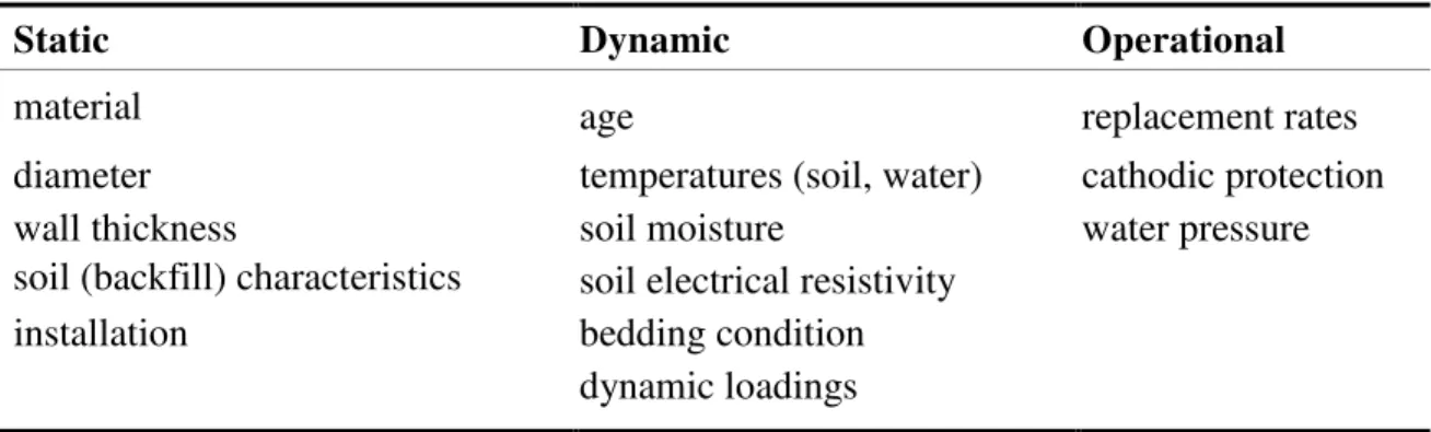
Typically, water mains break when environmental and operational conditions exert stresses that exceed their diminishing structural resiliency. The deterioration of pipes can be affected by operational and environmental conditions, some of which are static while others vary over time. Table 1 lists the main factors that may affect pipe breakage rates. It can be seen that the factors that are static over time generally relate to the properties of the pipe and installation practice, whereas the dynamic factors are those surrounding the pipe and its environment. Soil, being a static medium is somewhat of an exception, but many of the soil properties are dynamic, including temperature, moisture, electrical resistivity (varies due to moisture fluctuations and de-icing salts), among others.

Table 1. Factors affecting pipe breakage rates.

Static Dynamic Operational

material _{age replacement rates}

diameter temperatures (soil, water) cathodic protection wall thickness soil moisture water pressure soil (backfill) characteristics soil electrical resistivity

installation bedding condition dynamic loadings

Several researchers (e.g., Newport 1981; Walski and Pelliccia 1982; Lochbaum 1993) observed the effects of temperature and/or moisture conditions on the breakage rate of water mains. Yet, most breakage prediction models in water mains developed so far deal almost exclusively with static factors. The reason for that could be twofold. First, the modelling of some of those time-dependent factors, e.g., soil resistivity require extensive amounts of data that are historically unavailable and costly to acquire. Second, many undoubtedly question the merit of using effects like temperatures in breakage prediction models, seeing that temperatures in themselves can not be predicted reliably.

Availability of data not withstanding, ignoring time-dependent factors in any statistical analysis of break rates may yield biased results in many cases. Conceptually, pipe breakage rate can be viewed as a non-decreasing function of time (disregarding, for simplicity, phenomena like the first phase of the bathtub effect), with “noise” that is superimposed upon it by time-dependent effects. Some of these time-time-dependent factors are steady while others are transient or cyclical in nature. Cyclical effects tend to average out in the long run, however, when dealing with short data sets the cyclical effects can introduce significant bias into analysis results. In this paper a case study is used to demonstrate how breakage prediction models can consider time-dependent factors in order to refine the accuracy of their predictions. The factors considered in this case study are: operational – water main replacement rates and cathodic protection, and environmental – temperatures and soil moisture.

Temperature and soil moisture effects

The influence of temperatures on water and gas main breakage rates was observed by others, e.g., Lackington and Large (1980), Newport (1981), Needham and Howe (1981), Walski and Pelliccia (1982), Cittoni (1985), Goulter and Kazemi (1989), Lochbaum (1993), Habibian (1994), Chambers (1994), and others. Most of them reported typical annual patterns of breakage rates that peak during or towards the end of the winter season, when the ground temperatures are the lowest.

The influence of soil moisture on breakage rates of water and gas mains was observed by Baracos et al. (1955), who reported that water main breaks in Winnipeg occurred largely between September and January and peaked especially under dried-soil conditions after a hot summer or just prior to spring thaw. Morris (1967) and Clarke (1971) reported that volumetric

swelling and shrinkage of clays is also a factor that contributes to a high number of water main breaks. Newport (1981) observed peaks in breakage rates following very hot and dry summers in the UK. Hudak et al. (1998) also observed that extreme dry periods led to an increase in water main breaks in expansive soils found in Texas, USA.

Rajani et al. (1996) developed a pipe-soil interaction model, which demonstrates how temperature and soil moisture interact to influence pipe breakage rate. Buried mains are restrained from movement by the frictional resistance between pipe and soil. Pipes that were initially installed at a warm ambient temperature will contract (axially and to a minor extent circumferentially) upon subsequent drop in water and ground temperatures, resulting in the development of axial tensile stresses. Conversely, tensile stresses in the pipe can also be induced if pipes attempt to resist deformation imposed by soil shrinkage as moisture is depleted.

Rajani and Zhan (1996) developed a model to describe the mechanics and circumstances that lead to the generation of frost loads. These loads develop primarily as a consequence of different frost susceptibilities (frost penetration and frost heave) of trench backfill and sidefill (native soil) and the interaction at the trench backfill-sidefill interface. The depth of the frost front can be estimated using the Berggren function (Aldrich 1956), which considers thermal properties of the unfrozen and frozen soil, freezing index and latent heat of the frozen soil. The Berggren function shows that dry soil (expected after an extreme dry season) will have low latent heat capacity and will therefore lead to deeper frost penetration even if the thermal conductivity and freezing index remain unchanged.

Clays with high montmorillonite mineral content can undergo substantial volume change when subjected to seasonal wet (swelling) and dry (shrinkage) conditions. However, a physical model of how these volume changes impose stresses on the pipes is not currently available. Nonetheless, longitudinal and vertical actions are likely to compound and lead to a water main break whenever processes like corrosion have compromised the structural resiliency of the main.

Time-dependent modelling of water main break

In a recent review (Kleiner and Rajani, 2001), the statistical methods available in the literature to predict water main breakage were classified broadly into deterministic, probabilistic multi-variate and probabilistic single-variate models applied to grouped data. The statistical methods for predicting water main breaks use available historical data on past failures to identify

pipe breakage patterns. These patterns are then assumed to continue into the future in order to forecast the breakage rate of a water main or its probability of breakage. Of all the statistical methods reviewed, none considered time-dependent variables other than pipe age and sometimes the number of previous breaks. Mathematically, time-dependent variables could be considered in most existing models, though in some cases the statistical analysis might prove to be substantially more challenging. This paper focuses on the time-exponential models to predict breakage rates. A desirable precursor to this type of statistical analysis is to partition the population of water mains into groups that are appreciably uniform and homogeneous with respect to their response to deterioration and stress inducing mechanisms. Grouping criteria could be properties such as material type, pipe size, vintage, soil type, etc. These time-exponential models have been quite popular and in several cases have been used to analyse large distribution systems (e.g., Walski and Pelliccia,1982; Walski and Wade, 1987; Male et al., 1990; Kleiner and Rajani, 1999).

Time-exponential model

Shamir and Howard (1979) were the first to suggest that water main breakage rates increased exponentially with pipe age.

) ( 0 0 ) ( ) (t N t eAt t N = − (1)

where t is the elapsed time (from a reference year to for which the breakage rate is known) in years; N(t) is the number of breaks per unit length per year (km-1 year-1) at time t, and A is the coefficient of breakage rate growth (year-1).

This single variate, two-parameter expression was used by many others with and without modifications, e.g., Walski and Pelliccia (1982), Clark et al. (1982), Kleiner et al. (1998), Kleiner and Rajani (1999) to name a few. This expression can be generalised it to a multi-variate exponential model T t x a t N x e x N( )= ( t₀) ⋅ (2)

where xt = vector of time-dependent covariates prevailing at time t, N(xt) = number of breaks

resulting from xt, a = vector of parameters corresponding to the covariates x, and x_t0 = vector of

could be pipe age, temperature, soil moisture, etc. Parameters N

( )

0 t

x and a can be found by least

square regression (with or without linear transformation) or by using the maximum likelihood method. A similar approach can be used to extend the time-power function, as suggested by Constantine and Darroch (1993), to a multi-variate power model.

It should be stressed that equation (2) in its current form should be applied to groups of pipes that are relatively homogeneous with respect to their response to the selected set of covariates. The criteria of grouping the pipes into homogeneous groups can be unique to a distribution system and is often not known a priori. The time-dependent factors that were examined for this study were:

• underlying ageing effects, expressed as time elapsed from a baseline year, which is the first year that breakage data were available;

• temperature effects, expressed as the freezing index;

• soil-moisture effects, expressed as the rainfall deficit;

• cumulative length of replaced water mains, expressed as a percentage per year of the total inventory analysed;

• cumulative length of cathodically protected (retrofitted) water mains, expressed as a percentage per year of the total inventory analysed.

The following is a description of these factors and the manner in which they were considered.

Freezing index (FI)

The freezing index provides a measure of the severity of winter during a specified period. It was selected as a surrogate measure for temperature effects on water main breaks following many reported observations of increased breakage rates in cold winters The periodical freezing index is expressed in degree-days, which is the cumulative average daily temperature below a threshold temperature τ [OC] during a given period:

å

τ

In this study the actual FI covariate was taken as the Z score of the freezing index, namely the FI values were normalised by their mean and standard deviation according to

) ( ) ( ) ( FI SD FI mean FI FI score Z = − (4)

in order to obtain a better stability in the calculations as well as obtain non-dimensional parameters that are comparable in orders of magnitude.

Rain deficit (RD)

Soil moisture conditions are difficult to quantify directly because of the spatial variations in soil types and precipitation rates to which water distribution systems are subject. The Thornwaite method (e.g., Withers and Vipond 1980) for quantifying rain deficit was selected as a surrogate for soil moisture. It quantifies the moisture depletion in the ground as a function of temperature, precipitation and geographical latitude. While there are other, sometimes more refined, methods to quantify soil moisture, the Thornwaite method was selected because of its simplicity and the ease of obtaining the required data. This method was developed in the Eastern USA. It is more suitable to humid climates, and therefore requires some modification for other climates. The effect of these modifications on the results are deemed minimal because the time-dependent relative variations in soil moisture are of interest rather than their absolute values. The RD was also normalised by its mean and standard deviation according to (5) for the same reasons as the

FI covariate. ) ( ) ( ) ( RD SD RD mean RD RD score Z = − (5)

As previously described, low soil moisture levels may affect pipe breakage rates in two ways. In dry seasons low soil moisture contributes to soil shrinkage, and in cold seasons to increased frost penetration. Consequently, the rainfall deficit (RD) factor was considered in two ways. Its contribution to soil shrinkage in a given year was represented by the average RD for the year, which is a measure of how dry the year was. Its contribution to frost penetration was represented by a snapshot of the rain deficit at the beginning of winter (typically end of November). It was assumed that in cold regions the soil moisture is roughly constant during winter due to the predominantly frozen conditions of the soil.

Cumulative length of replaced mains (CLR)

In many models of main breaks, the number of breaks are normalised by the total length of the water main in the inventory, resulting in units of number of breaks per pipe length. This practice is instrumental as water main inventories change over time due to new construction and/or abandonment. However, it also implies that the spatial distribution of the breaks along the pipes is uniform. This implication may bias the model, especially when implementing a replacement program for water mains, in which the mains with the highest breakage rates are typically replaced first. Taking the cumulative length of the mains replaced (CLR) as an additional time-dependent covariate may capture this phenomenon. Specifically, it was assumed that the CLR in year i would affect the breakage rate in year i+1. The units for CLR were taken as the cumulative percentage of water main length replaced.

Utilities that keep detailed inventories, in which every break is attributed to a specific pipe, can perform the multivariate analysis (equation (2)) on groups of pipes that have not yet been replaced. In such case there is no need to consider CLR explicitly in the model (for a group containing un-replaced pipes the CLR is in fact zero).

Cumulative length of cathodic protection (CLCP)

There is evidence that pipes that have been retrofitted with cathodic protection change their deterioration patterns in certain circumstances (e.g., Gummow 1988; Doherty 1990; Green et al. 1992). Similar to CLR, the pipes that are likely to receive this retrofit first are the ones with the highest breakage rates. Thus, the cumulative length of cathodically protected pipes (CLCP) was also taken as a time-dependent covariate where applicable. Actual units used were the cumulative percentage of water main length that was protected. This assumption implies that the cathodic protection is well maintained and that expired anodes are replaced in a timely manner.

Illustrative example - Ottawa

Breakage analysis

The data set for cast and ductile iron mains (up to 12” diameter) from the region of Ottawa-Carleton (referred to as Ottawa in the rest of the paper), Ontario, contained records of monthly water main breaks, as well as length of pipe replaced and cathodically protected for the years 1973-98. As will later be discussed, it would have been preferable to analyse cast and ductile iron separately, however, data attributing breaks to specific types of pipe were not available

(ductile and cast iron pipes comprise about 95% of total inventory). In 1987 the utility embarked upon an aggressive main replacement program and in 1994 a program of cathodic protection retrofits was initiated. The climate data was obtained from Environment Canada. In accordance with the discussion presented earlier in the section on Temperature and soil moisture effects, it was assumed that:

• A warm and dry summer with a relatively high rainfall deficit (RD) will tend to increase the breakage rates of the following winter, because low soil moisture content will decrease the latent heat capacity that mitigates frost penetration.

• A cold winter will tend to increase the breakage rate because of increased frost penetration. The threshold temperature to calculate FI was taken τ = 0OC

• A relatively warm and dry year will tend to increase breakage due to shrinkage of clayey soils.

• In Ottawa, the soil is, for the most part, frozen during winter (December-April) at the relevant depths, therefore the value of the RD in at the end of November was taken as the “snapshot” value.

As a consequence of these assumption, it was computationally convenient to take the basic time-step as the twelve-month period May-April rather than the 12-month calendar year (January to December) in order that the end of winter coincide with the end of the time-step unit.

Equation (2) was applied to the data in various ways to demonstrate how the inclusion of different covariates influences the analyses. These results are shown in Table 2 and illustrated in Fig. 1. F-statistics, t-statistics and coefficients of determination (simple r2 as well as adjusted ra2)

Fig. 1 Main break rate as a function of time, FI, RD (Cases 1 and 2). (a): case 1 (b): case 2 0 200 400 600 1970 1975 1980 1985 1990 1995 2000 2005 Year Br e a k s Observed Predicted Background ageing 95% confidence CP program Replacement program (c): case 3 0 200 400 600 1970 1975 1980 1985 1990 1995 2000 2005 Year Br e a k s Observed Predicted Background ageing 95% confidence CP program Replacement program 0 200 400 600 1970 1975 1980 1985 1990 1995 2000 2005 Year Br e a k s Observed Predicted Background ageing 95% confidence CP program Replacement program

Table 2. Coefficients for Ottawa water main breakage data.

Variable Case 1 Case 2 Case 3 Case 4 Case 5 Case 6

N xoc h

- breaks/km 0.054 0.048 0.048 0.049 0.049 0.047

Ageing rate for old pipe 0.027 0.032 0.032 0.031 0.031 0.033

Cathodic Protection (CLCP) -7.305 -9.255 -8.093 -8.477 -6.975

Rainfall deficit (RD) - cumulative 0.060 0.063 0.069 0.069

Freezing index (FI) 0.032 0.030 0.032

Rainfall deficit (RD) - snapshot 0.022 0.022

Length replaced (CLR) -1.898

Co

ef

ficien

ts

Simple coefficient of determination (r2) 0.619 0.703 0.763 0.776 0.787 0.793

Adjusted coefficient of determination (ra2) 0.603 0.679 0.732 0.736 0.736 0.731

Regression F-statistic 48.520 29.187 23.757 18.292 14.459 11.583

Critical F value at 95% confidence 4.242 3.403 3.028 2.817 2.685 2.599

Statistical significance (t-ratio)

N xoc h - breaks/km 0.000 0.000 0.000 0.000 0.000 0.000

Ageing rate for old pipe 0.000 0.000 0.000 0.000 0.000 0.000

Cathodic protection (CLCP) 0.057 0.015 0.038 0.034 0.218

Rainfall deficit (RD) - cumulative 0.046 0.038 0.031 0.035

Freezing index (FI) 0.281 0.323 0.312

Rainfall deficit (RD) - snapshot 0.460 0.471

Pipe replacement (CLR) 0.706

P-valu

e

A word of caution is warranted about the interpretation of the results in Table 2. For F-statistics and t-statistics to be valid, it is required that the error term be additive, independent and normally distributed with a mean of zero and a variance σ2. The F-statistics and t-statistics values in Table 2 pertain to a (linear) regression that was performed on Equation(6), which is a linearised version of Equation (2), with explicit error terms εt . Equation(6) implies that the error

terms are multiplicative in the original (exponential) space. These εt are assumed to be normally

distributed with a mean of zero and a variance σ2, however, this assumption should be treated with caution, given the nature of the data (repeat measurements not possible – only one response per year) and the number of data points available. The 95% confidence interval was constructed in the linearised space under these assumptions.

t T t t N x a x x N( )]=log[ ( )]+ ⋅ +ε log[ t₀ (6)

The adjusted ra2 is the coefficient of determination adjusted to account for the loss of one

degree of freedom for every additional covariate used. It is less restrictive than F-statistics and t-statistics because it does not require that the error be normally distributed around the regression line. It can also be performed directly on the (original) exponential space rather than on the linearised space, with the assumption that the error terms are additive rather than multiplicative. In Table 2 both the simple and adjusted ra2 are those resulting in the exponential space – for

comparison. The regression analysis was performed with all combination and permutations of the covariates and the order (left to right) in Table 2 reflects their respective significance.

Case 1 (Fig. 1a) demonstrates the customary (time only) analysis. This analysis implies that only steady state ageing is responsible for the variations in break rates. All indicators in Table 2 suggest that indeed ageing has a statistically significant (better than 99% confidence level) influence on breakage rates in Ottawa, and that this high significance is independent of any other covariate. The positive sign of the coefficient indicates, as expected, that ageing increases breakage rate.

Case 2 (Fig. 1b) considers the addition of cumulative length of cathodic protection (CLCP). This covariate seems to well capture the downturn in breakage rate apparent in recent years. It

contributes significantly to the improvement in Ra2 (from 0.603 to 0.679) and is statistically

significant at better than 94% confidence level. It should also be noted that its inclusion changed the ageing coefficient from 0.027 to 0.032, suggesting that the true ageing rate was masked by cathodic protection. The negative sign of the CLCP coefficient indicates, as expected, that the more pipes are retrofitted with cathodic protection the smaller their breakage rate.

Case 3 (Fig. 1c) adds cumulative rainfall deficit (RD) into the model. This covariate improves in Ra2 (from 0.679 to 0.732) and is statistically significant at a higher that 95%

confidence level. Ottawa’s soils comprise a significant amount of Leda clay, which is characterised, among other things, by a strong tendency to shrink under dry conditions. Since the cumulative RD covariate measures average soil moisture conditions throughout the year, this could explain it’s relatively high and statistically significance influence on water main breakage rates, in particular explaining the year-to-year variation in the number of water mains breaks. The positive sign of the coefficient indicates, as expected, that the higher the RD the higher the breakage rate.

Case 4 adds freezing index (FI) to the model. It can be seen that its contribution to the improvement of Ra2 (from 0.732 to 0.736 at about 72% confidence level) is statistically

insignificant. It should be remembered that the adjusted ra2 pertains to the original (exponential)

space, while the t-statistics pertain to the linearised space, thus, this apparent conflict should be subject to judgement call. A plausible reason for FI having such a minor influence on breakage rate in Ottawa is that the typical depth of water mains is 2.4 m (8 feet), which attenuates much of the frost penetration. The positive sign of the coefficient indicates, as expected, that the higher the FI the higher the breakage rate.

Case 5 indicates that covariate snapshot RD appears to be statistically insignificant, both according to its t-ratio and contribution to the adjusted ra2. The snapshot RD measures the

antecedent conditions of winter soil moisture, which are assumed to exasperate frost penetration effects. The typical high depth of water mains in Ottawa may be a possible explanation to the low significance of this covariate. The positive sign of the coefficient indicates, as expected, that the higher the FI the higher the breakage rate.

Case 6 indicates that covariate pipe replacement (CLR) is also statistically insignificant in “explaining” breakage rates. This could be attributed to various reasons. Firstly, CLR is highly correlated with CLCP. This co-linearity manifests itself not only in high P-value for CLR but also in a degradation of P-value for the CLCP covariate (from 0.034 to 0.218) when CLR is added to the regression. When CLR replaces CLCP in case 2 it does contribute to increase the adjusted ra2 (from 0.603 to 0.661) and its P-value reduces to 0.130. This would indicate (albeit

with relatively low statistical significance of 87%) that pipe replacement does affect breakage rate, although maybe the pipes that have been replaced were not always those which subsequently failed more frequently. Another explanation could be that the assumption, that pipes replaced at year t would reduce breakage rate at year t+1, is inaccurate, and that in fact a longer time-lag exists. The negative sign of the CLR coefficient indicates, as expected, that the more pipes replaced the smaller the breakage rate.

It should be mentioned that in some cases, when a historical data set is short and includes a period in which breakage rates predominantly decrease, the multi-variate exponential model may yield results that are counter-intuitive, such as positive effect of ageing and/or negative effects of replacement. A possible approach to prevent this phenomenon is to apply constraints for the coefficients CLR and CLCP in the solution process. These constraints, however, have two minor shortcomings; they complicate the mathematical solution and, they may mask a (unlikely, though possible) case in which a utility is targeting the wrong pipes in its replacement or cathodic protection programs (thus increasing average breakage rate instead of reducing it).

Forecasting water main breaks in the short-term

Forecast of climatic factors

As was described in the introduction, long-term planning of water main renewal is primarily concerned with background ageing of pipes (obtained after filtering out time-dependent “noise), whereas short-term planning is concerned also with the time-dependent cyclical variations. The climatic effects influencing pipe breaks need to be forecasted in order to predict frequencies of breakage in the near future. If a water utility has access to elaborate climate forecasts (e.g., by local climate centres), it can use them to forecast FI and RD in the near future in order to predict water main breaks. When elaborate climate forecasts are unavailable a “do it yourself” approach

could be used, in which utilities can compile their own forecasts by applying a relatively simple Fourier analysis to historical temperature and precipitation data that are often available locally.

Climate prediction (Lorenz 1975) is the process of determining how atmospheric statistics gathered over a given averaging period (typically several years or longer) evolve over longer time frames. Climate differs from weather in that it provides a statistical view of seasonal and daily weather events over a long-term period. Forecasting climate with models is well recognised as a difficult endeavour because these models need to consider processes with very large spatial scales (such as transport of energy from the tropics to the poles by atmospheric motions) as well as small-scale processes (such as collection of water molecules into raindrops). It is not the purpose of this paper to offer a comprehensive review of climate models but to provide sufficient details for the reader to readily follow the general notions of the approach taken here.

Climate-prediction models can broadly be classified into “physical” and “stochastic.” Circulation models (Boer et al. 1984) are an example of physical models. They discretise earth’s surface into a grid and then assign average properties to each point on the grid using accepted laws of physical processes such as solar and terrestrial radiation, horizontal large-scale flow, precipitation, latent heat release, surface energy balance and hydrology. Full climate models consider processes occurring in large domains, both spatial (landmasses, oceans, atmosphere) and temporal. For example, interannual to multi-decadal variations in the climate system are related to coupled atmosphere-ocean mechanisms. Some of these mechanisms have been identified such as the El Niño-Southern Oscillation (ENSO) phenomenon, the Quasi-biennial Oscillation, monsoonal dynamics, and decadal scale circulation oscillations such as that found in the North Atlantic. To be considered valid, a physical-class climate model must be able to reproduce observed climate in both time and space, and must do so by considering all these various processes while maintaining proper relationships among various parts of the climate system

An alternative approach for predicting climate is to use stochastic models that focus on general phenomena rather than specific observations in time and space. For example, stochastic models can be used to determine whether the mean and variance of cold temperatures are large during several winter seasons and to describe the impact of this trend on the overall pole-ward transport of heat in both the atmosphere and ocean. Simplified stochastic modeling for climate has emerged from work done by Hasselman (1976) and Leith (1975).

In this paper, the two climate variables of interest for the time-dependent analysis of water main breakage are precipitation (contributing to rainfall deficit) and temperature (contributing to both rainfall deficit and freezing index). Water mains are buried in the ground, which is a medium of enormous capacity for both heat and moisture. This capacity attenuates short-term variations in both moisture input (precipitation) and temperature input (air temperature). Consequently, variations in monthly and annual averages are of interest. The approach described here is to analyse the historical climate time-series data using Fourier analysis. This form of analysis breaks the data into separate harmonic components under the assumption that climate events are harmonic. The assumption of harmonic weather components is controversial in light of recent evidence of global climate change. It could however be argued that this climate change is in itself a low-frequency harmonic phenomenon, which was not observed earlier because available data did not extend far enough into the past. Further, Fourier analysis can be modified to extract the underlying trend (if known) as well as harmonic components.

Fourier analysis

Fast Fourier Transform (FFT) converts data from the time domain into the frequency domain. The discrete form of the Fourier series for any time series (x(t)) can represented by:

x t a_o a_k t b t

k M

k

b g= +2

å

where t is time, M is equally spaced sample data in the time series, T (=2πk/ω) is the period, ω is the frequency, k is the frequency number, and ak and bk are the Fourier coefficients. The time

series x(t) can represent time-dependent variables such as precipitation or temperature. The issue of underlying long-term trend in the data is not of concern here because such a trend is not likely to have an effect on near-term forecasts. Details on the application of the fast Fourier transform will not be described here as it is explained in several textbooks, e.g. Newland (1993).

Climate forecast

Prior to describing how climate was forecast for Ottawa, it should be reiterated that the FFT procedure to model climate is provided only as a rudimentary tool intended as a fast alternative for those who have no access to a more robust climate forecast (e.g., from a local weather bureau).

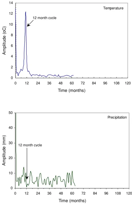
Temperature and precipitation data for the years 1973-98 for Ottawa were obtained from Environment Canada. The Fourier amplitude spectra for these data are shown in Fig. 2. The temperature spectra (Fig. 2a) clearly show the expected annual (12-month) cycle as the predominant one. The precipitation spectra (Fig. 2b) however, are much less definite, showing no particular dominant frequency.

The forecasting of temperature and precipitation was conducted in three stages, model fit, validation (holdout sample) and forecasting, as shown in Fig. 3. Historical data were partitioned into two groups, the modelling sample, comprising data from April 1986 to November 1997 (a total of 27 = 128 data points), and the holdout sample with data from December 1997 to January 1999. Fourier analysis was conducted on the modelling sample, and prediction models were derived for temperature and precipitation. Subsequently, these models were used to forecast temperature (Fig. 3a) and precipitation (Fig. 3b) for the holdout sample data of 25 months and the forecasts were compared to the observed data for validation. The results show good forecasting ability for temperatures (ra2 = 0.988).

Fig. 2 Amplitudes and frequency spectra for monthly temperature and precipitation in Ottawa. Precipitation 0 10 20 30 40 50 0 12 24 36 48 60 72 84 96 108 120 Time (months) A m p lit ud e ( m m ) Temperature 0 2 4 6 8 10 12 14 0 12 24 36 48 60 72 84 96 108 120 Time (months) A m p lit ud e ( oC ) 12 month cycle 12 month cycle (a) (b)

Fig. 3 Validation and forecast of temperature and precipitation in Ottawa, using Fourier analysis

Modelling sample (Fourier analysis) Validate Forecast sample

Modelling sample (Fourier analysis) Validate

sample Forecast (b) (a) -30 -20 -10 0 10 20 30 96 120 144 168 192 216 240 264 288 312 336 360 Time (months) T e mper atur e ( o C ) Temp. observed

FFT fit Modelling sample (Fourier analysis)

Holdout sample Forecast -50 0 50 100 150 200 96 120 144 168 192 216 240 264 288 312 336 360 Time (months) P re c ip ita tio n ( m m ) Precip. observed

FFT fit Modelling sample (Fourier analysis)

Holdout

It appears that in Ottawa average monthly temperatures are quite predictable due to the clear and dominant 12-month cycle (as evident in Fig. 2a) plus some other very minor cycles. Precipitation, however, appears to be difficult (ra2 = -0.536) to forecast due to its relatively uniform frequency

spectra (Fig. 2b), which indicate no dominant harmonic pattern. This difficulty may be peculiar to the cool, wet climate of Ottawa and may not be encountered in other climates (the same analysis in Edmonton, Alberta, produced a much better forecast). Fourier transform analysis is highly debated by climatologists because climate is not widely accepted to be a harmonic process. Hence, the approach proposed here should be used as a “starting point” for generating a “bottom up” forecast.

Subsequently temperatures and precipitation were forecast for the 4 years (1999 – 2002), for which no data were available at the time of analysis. Rain deficit (RD) and freezing index (FI) were then calculated for these years.

Forecasting water main breaks

Using RD and FI, forecasted for the years 1999 – 2002, water main breaks were predicted for these years. It should be stressed that at the time of analysis break data for 1999-2000 were not available. Break data for these two years (and the first 3 months in 2001) were obtained only after forecasting was implemented, thus in effect, years 1999 and 2000 served to validate part of the forecasting.

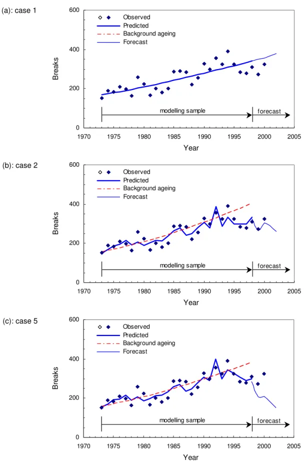
Fig. 4a shows the forecast of water main breaks when neither climate nor operational are considered. Fig. 4b shows the forecast that considers time, FI, RD, and CLR that includes 1% replacement rate per year. Fig. 4c shows the forecast that accounts for all factors, including time, FI,

RD, and CLR (1% per year) and CLCP of 2% per year. It is evident that the forecast is most accurate

when replacement rate (CLR) is considered without cathodic protection (CLCP), as indicated in Fig. 4b. This could be due to reasons discussed already in Section Breakage analysis, namely the fact that cathodic protection retrofit started only in the last five years of the data set, and the co-linearity between the CLCP and CLR variables.

2

Fig. 4 Short-term forecasts of water main break rate (Cases 1, 3 and 5).

0 200 400 600 1970 1975 1980 1985 1990 1995 2000 2005 Year B reak s Observed Predicted Background ageing Forecast forecast modelling sample 0 200 400 600 1970 1975 1980 1985 1990 1995 2000 2005 Year Br e a k s Observed Predicted Background ageing Forecast forecast modelling sample (b): case 2 (a): case 1 (c): case 5 0 200 400 600 1970 1975 1980 1985 1990 1995 2000 2005 Year B reak s Observed Predicted Background ageing Forecast forecast modelling sample

3

Forecasting water main breaks in the long-term

As discussed in the introduction, the long-term planning of water main renewal requires accurate quantification of the underlying rates of ageing of water mains in order to identify the time at which it is more economical to replace than to continue repairing the pipe. The “true” underlying ageing rate can often be masked by time-dependent factors. The proposed approach can help filter out these effects in order to obtain a more accurate estimate of the ageing rate. For example, the ageing rate coefficient in cases 3 is 0.034 (Table 2) compared to 0.029 in cases 1 and 2. This clearly demonstrates that cathodic protection masked the true ageing rate of the water mains in this example. It is interesting to note that climatic covariates did not mask the true ageing rate likely because in relatively long data sets cyclical environmental effects tend to average out around the ageing trend. However, these cyclical environmental effects could significantly mask the ageing trend when the available data set is relatively short. Kleiner and Rajani (1999) demonstrated this phenomenon by comparing ageing trends obtained from sub-sets (10 years) of data, with and without considering RD and FI, to those obtained from a complete data sets (37 years) from Edmonton, Alberta, Canada.

It should be noted, however, that this “unmasking” is not always possible. If a short data set contains some conflicting signals, or if some fundamental conditions change over a period that is not long enough to establish consistency (e.g., a cathodic protection program was started in the last year or two of the data set), then the results could be invalid. The model should be used judiciously and the outcome of the analysis interpreted with caution.

Summary

Planning for water main rehabilitation and renewal is imperative to meet adequate water supply objectives. The ability to understand and quantify pipe deterioration mechanisms is an essential part of the planning procedure. While a comprehensive physical model of pipe deterioration is desirable, it is currently more realistic to use statistical models for distribution water mains due to the unavailability and the cost of acquiring data necessary for physical models. Over the last two decades various models have been developed to statistically model and predict pipe failures and failure rates. These models, however, have dealt predominantly with static, rather than time-dependent, factors, which influence the breakage of water mains.

4

A new method has been presented in which time-dependent factors can be considered in the statistical modelling breakage rates for water mains. This method, which can be applied either as a multi-variate exponential model or a multi-variate power model is powerful, yet simple enough to account for ageing as well as environmental and operational effects that vary over time. The application of this method was demonstrated with the thorough analysis of data from Ottawa, Ontario, that considered ageing, as well as environmental (FI, RD) and operational (CLR, CLCP) time-dependent variables. Other variables can be considered if they are judged to be significant and if relevant data are available.

The application of time-exponential multivariate model was used to make short-term (3 to 4 years) forecasts for the number of water main breaks. Forecasted climate data required for this multivariate model was obtained from Fourier analysis, which assumed that climate change follows harmonic cycles. Alternatively, forecasts of climate available from climate centres around the world could be used. The analysis was validated by comparing forecasted climate with observations in Ottawa and agreement was quite good.

In the long-term planning of water main renewal, the method can be used to obtain more accurate estimates for pipes of the underlying ageing trends, which can be masked by time-dependent effects, especially in short data sets.

The consideration of time-dependent factors can be incorporated in existing break prediction models (e.g., proportional hazards, accelerated life time, and others) to improve their accuracy and to remove possible biases.

Acknowledgements

We would like to extend our gratitude to the water utilities of Adelaide (Australia), Edmonton (EPCOR Water Services) and the Regional Municipality of Ottawa Carleton for providing the data for this research.

5

References

Aldrich, H. P. (1956). “Frost penetration below highway and airfield pavements.” Highway

Research Board, 36(145), 125-144.

Baracos, A., Hurst, W. D., and Legget, R. F. (1955). “Effects of physical environment on cast iron pipe.” J. AWWA, 47(12), 1195-1206.

Boer, G. J., McFarlane, N.A., Laprise, R., Henderson, J. D., and Blanchet, J. P. (1984): “The Canadian climate centre spectral, atmospheric general circulation model.”

Atmosphere-Ocean, 22(4), 397-429.

Chambers, G. M. (1994). “Reducing water utility costs in Winnipeg.” Proceedings of the Western

Canada Water and Wastewater Association Conference, October, Winnipeg, Manitoba. pp.

1-12.

Ciottoni, A. S. (1985). “Updating the New York City water system.” Proceedings of the Specialty

Conference on Infrastructure for Urban Growth. pp. 69-77.

Clark, C. M. (1971). “Expansive-soil effect on buried pipe.” J. AWWA, 63, 424-427.

Clark, R. M., Stafford, C. L., and Goodrich, J. A. (1982). “Water distribution systems: A spatial and cost evaluation.” J. Water Resources Planning and Management Division, ASCE, 108(3), 243-256.

Constantine, A. G., and Darroch, J. N. (1993). “Pipeline reliability: stochastic models in engineering technology and management.” S. Osaki, D.N.P. Murthy, eds., World Scientific Publishing Co.

Doherty, B. J. (1990). “Controlling ductile-iron water main corrosion: A preventive maintenance measure.” Materials Performance, 29(1), 22-28.

Green, B. M. Johnson, F. and De Rosa, J. (1992). “In situ cathodic protection of existing ductile iron pipes.” Materials Performance, 31(3), 32-38.

Goulter, I. C., and Kazemi, A. (1988). “Spatial and temporal groupings of water main pipe breakage in Winnipeg.” Canadian J. Civil Engrg., 15(1), 91-97.

Gummow, R. A. (1988). “Experiences with water main corrosion.” Joint Annual Conference of the

6

Habibian, A. (1994). “Effect of temperature changes on water-main break.” J. Transportation

Engrg., ASCE, 120(2), 312-321.

Hasselman, K. Stochastic climate models. Part I: Theory. Tellus 28 (1976), 473-485.

Hudak, P., Sadler, B. and Hunter, B. (1998). “Analyzing underground water-pipe breaks in residual soils.” Water/Engineering Management, 145(12), 15-20.

Kleiner, Y., Adams, B. J., and Rogers, J. S. (1998). “Long-term planning methodology for water distribution system rehabilitation.” Water Resources Research, 34(8), 2039-2051.

Kleiner, Y., and Rajani, B. B. (1999). “Using limited data to assess future need.” J. AWWA, 91(7), 47-62.

Kleiner, Y., and Rajani, B.B. (2000). “Considering time-dependent factors in the statistical prediction of water main breaks.” Proc., American Water Works Association Infrastructure

Conference, Baltimore.

Kleiner, Y and Rajani, B. B., (2001). “Comprehensive review of structural deterioration of water mains: Statistical models”, To be publishe in J. Urban Water in December2001.

Lackington, D. W., and Large, J. M. (1980). “The integrity of existing distribution systems.” Journal

of the Institute of Water Engineers and Scientists, 34,15-32.

Leith, C. E. (1975). “Climate response and fluctuation dissipation.” J. Atmos. Sci., 32, 2022-2025.

Lochbaum, B. S. (1993). “PSE&G develops models to predict main breaks.” Pipeline and Gas J., 20(9), 20-27.

Lorenz, E. N. (1975). “Climate predictability: In the physical basis of climate and climate Modelling.” Global Atmospheric Research Programme Publication No. 16, pp. 132-136. World Meteorological Organization, Geneva.

Male, J. W., Walski, T. M., and Slutski, A. H. (1990). “Analysing watermain replacement policies.”

J. of Water Resources Planning and Management, ASCE,116(3), 363-374, May/June.

Morris, R. E. (1967). “Principal causes and remedies of water main breaks.” J. AWWA, 54, 782-798.

7

Newland, D.E. (1993). “An introduction to random vibrations, spectral and wavelet analysis.” John Wiley, New York. 3rd Ed.

Newport, R. (1981). “Factors influencing the occurrence of bursts in iron water mains.” Water

Supply and Management, 3, 274-278.

Rajani, B., and Zhan, C. (1996). “On the estimation of frost load.” Canadian Geotechnical J., 33(4), 629-641.

Rajani, B., Zhan, C., and Kuraoka, S. (1996). “Pipe-soil interaction analysis for jointed water mains.” Canadian Geotechnical J., 33(3), 393-404.

Shamir, U., and Howard, C. D. D. (1979). “An analytic approach to scheduling pipe replacement.” J.

AWWA, 71(5), 248-258.

Walski, T. M., and Pelliccia, A. (1982). “Economic analysis of water main breaks.” J. AWWA, 74(3), 140-147.

Walski, T. M., and Wade, R. (1987). “New York Water supply infrastructure study.” Technical Report EL-87-9, US Army Corps of Engineers, July.

Withers B., and Vipond, S. (1980). “Irrigation: design and practice.” 2nd Edition, Cornell University

8

List of symbols

a vector of parameters corresponding to covariates x

ak, bk Fourier coefficients

A coefficient of breakage rate growth (in the 2-covariate equation) year-1

CLCP cumulative length of water mains cathodically protected – time-dependent covariate

CLR cumulative length of water mains replaced – time-dependent covariate

DDp degree days in period p or all the days with average temperature below 0OC. FI freezing index is expressed in degree-days – time-dependent covariate

k frequency number

M number of equally spaced sample data in the time series for climate

N(t) number of breaks per unit length at year t (in the 2-covariate equation)

N

( )

N(

( )

x _{number of breaks at baseline conditions at year of reference to} r2 coefficient of determination

ra2 adjusted coefficient of determination

RD rainfall deficit expressed in mm – time-dependent covariates (snapshot and cumulative)

to reference year

T period in Fourier analysis

Ti average daily temperature of day i

xt vector of time-dependent covariates prevailing at year t

0 t

x _{vector of baseline x values at year of reference to}