Music/fast, a pre-design and pre-mission analysis tool for the earth atmospheric re-entry of spacecraft, capsules and de-orbited satellites

To cite this version :

Sourgen, Frédéric and Prévereaud, Ysolde and

Vérant, Jean-Luc and Laroche, Emmanuel and Moschetta, Jean-Marc

MUSIC/FAST, A PRE-DESIGN AND PRE-MISSION ANALYSIS

TOOL FOR THE EARTH ATMOSPHERIC RE-ENTRY OF

SPACECRAFT, CAPSULES AND DE-ORBITED SATELLITES

.

(2015)

In: Proceedings of 8th European Symposium on Aerothermodynamics

for Space Vehicles, 2 March 2015 - 6 March 2015 (Lisbonne,

Portugal).

O

pen

A

rchive

T

OULOUSE

A

rchive

O

uverte (

OATAO

)

OATAO is an open access repository that collects the work of Toulouse researchers and

makes it freely available over the web where possible.

This is an author-deposited version published in :

http://oatao.univ-toulouse.fr/

Eprints ID : 14576

Any correspondance concerning this service should be sent to the repository

administrator:

staff-oatao@listes-diff.inp-toulouse.fr

MUSIC/FAST, A PRE-DESIGN AND PRE-MISSION ANALYSIS TOOL FOR THE EARTH

ATMOSPHERIC RE-ENTRY OF SPACECRAFT, CAPSULES AND DE-ORBITED

SATELLITES

F. Sourgen (1), Y. Prévereaud (1), J-L. Vérant (1) , E. Laroche (1), J-M. Moschetta (1)

(1)

ONERA, Midi-Pyrénées Center, BP 74025 – 2 avenue Edouard Belin, FR-31055 Toulouse cedex 4, Email:Frederic.sourgen@onera.fr

ABSTRACT

The paper proposes an overview of the physical models developed/selected and implemented in the ONERA aerothermodynamic (ATD) engineering code FAST. This tool is used to quickly determine the pressure and heat flux surface distribution at the wall, as well as aerodynamic forces and moments coefficients in hypersonic regime for free-molecular, transitional and continuum flows, for realistic designs of space vehicles ranging from capsules to spacecrafts and for generic shapes of orbital debris as well. An original feature of the approach is that geometrical components of the object are not separately processed but are investigated by a global method taking into account geometrical effects and flow history (shadow regions, surface heat flux propagation).

Several application cases are displayed to rely on the engineering approach: ARD and AOTV capsules, Pre-X (an IXV-like vehicle) and CubeSat (a debris-like single object). The given results have been analysed by comparison with experimental and CFD data. The limits of the approach are discussed, paving the way for future developments.

1. INTRODUCTION

The transport to space is a major discipline in current aerospace activities. Defining the right trajectory of a re-entry vehicle is crucial for the mission success. However, during the atmospheric re-entry, a strong interaction exists between ATD mechanisms, flight dynamics and vehicle shape. A predominant factor in designing a hypersonic re-entry vehicle is its shape: ranging from a ballistic flight design (e.g. Stardust, Mirca) providing aerodynamic stability, to semi-ballistic (Apollo, ARD, AFE) including guidance and control, and finally spacecraft configurations (Space Shuttle, PRE-X, IXV, HYPMOCES [1]) involving active trajectory and attitude control.

Therefore, during pdesign phase of atmospheric re-entry vehicles, several flight points, vehicle geometries and many configurations (rudders, wings positions and size, inflatable systems, flaps size…) have to be explored. CFD computations being cost-consuming in terms of CPU time and man labour, their number is limited in many projects. In addition, their use during the pre-design phase can turn out inappropriate

especially when the shape is not yet fixed. Therefore, engineering methods that are able to quickly and accurately compute aerodynamic forces and moments coefficients and heat flux distribution at wall are attractive tools.

Since 2006, ONERA has been developing a platform so-called MUSIC/FAST, which is the gathering of a multi-objects trajectory computation tool including GNC (MUSIC) [2] and a geometric treatment and aerothermodynamic modelling tool (FAST). MUSIC/FAST demonstrates an alternative but effective approach to CFD and GNC to prepare the pre-design phase of atmospheric re-entry vehicles within reliable estimates of aerodynamic forces and moments coefficients and wall heat flux distribution during 3DDL or 6DDL pre-flights within an attractive response time. This paper focuses on the aerothermodynamics modelling performed in the FAST code. First, the required geometrical treatment is described. Then, the following sections deal with aerodynamic coefficients determination in hypersonic regime for free-molecular, transitional and continuum flows. Thirdly, aerothermodynamic analysis (heating balance and heat flux models) is addressed. Then, three application cases are exhibited to rely on the engineering approach: ARD (Atmospheric Reentry Demonstrator) capsule, PRE-X, which is a IXV-like vehicle and CubeSat, which is an orbital debris-like single element. Along the paper, the given results are analysed by comparison with experimental and CFD data regarding aerothermodynamics, and the limits of the approach will be discussed, paving the way for future developments. Finally, in the last section an overview of an alternative model to the modified Newtonian method is proposed in the case of elliptic flows representation.

2. CAD ANALYSIS

Simple and more complex geometries can be designed and meshed with any CAD software. Geometries must be meshed with surface triangular mesh cells. From this, FAST computes automatically:

- the reference surface and length, used to compute aerodynamic forces and moments coefficients; - the local curvature radius used to compute the heat flux distribution at the wall.

of the centre of gravity of complex objects must be fixed by the user.

The local curvature radius model, developed at ONERA by Diallo [3], is based on the non-constraint divergent-gradient method. The local surface can be approximated by a quadric equation as following:

(1)

where x, y, z are the mesh surface coordinates. The coefficients from a to l are the unknown of the quadric equation. They are determined using local coordinates of neighbouring nodes. Then, the local curvature C and the local curvature radius r can be computed:

(2) Eq. 1 can be written for each node belongs to the first and second circles of neighbouring nodes of the considered node. A linear system with 10 unknowns and i equations (equal to the number of neighbours nodes considered) is obtained. In practice, a sufficient number of neighbouring nodes can always be found for the system to be solved.

Figure 1 displays the local curvature radius values computed on the ARD capsule following the above-mentioned method.

Figure 1. Computed curvature radius for the ARD capsule meshed with 13977 nodes.

3. AERODYNAMIC MODELLING

Forces and moments are deduced from local values of pressure and skin friction coefficients. Those depend on the flow regime, defined using the Mach number M and the Knudsen number Kn.

(3)

where λ is the mean free path (m), Lref the reference length of the vehicle (m), T∞ the temperature of the undisturbed flow (K), P∞ the upstream pressure (Pa), R the ideal gas constant (J/mol.K), NA the Avogadro’s number (mol-1), and σ the effective cross sectional area for spherical particles (m2).

The free-stream conditions are given by the US76 atmospheric model corrected by a Barlier model for altitudes above or equal to 120 km.

3.1. Continuum flow (Kn < 0.001)

In the continuum flow domain, a computation of the shock layer characteristics at stagnation point is performed under the thermochemical equilibrium hypothesis.

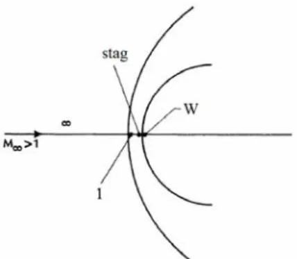
Given the flight point data, quoted “0” (or “∞”) in the figure 2, the shock layer values (quoted “1”) are obtained using Rankine-Hugueniot generalized equations, which can be written as following :

(4)

Gas are different upstream and downstream the shock (although they are assumed to be perfect gas), so that a chemical equilibrium table should be used. In FAST, the equations of Srinivasan et al. [4], which are valid for temperatures ranging between 0 and 25 000 K, are used.

Figure 2. The nomenclature for values behind the shock and at stagnation point [5].

The stagnation point values (“stag”) are obtained assuming isentropic compression of the gas from “1” :

(5) (6)

Those values are used as reference values in the following described models.

l iz hy gx fyz exz dxy cz by ax z y x F F x y z + + + + + + + + = = 2 2 2 ) , , ( , 0 ) , , ( + , r C=1/ =∇r⋅nr_F ) , , , y F y n =∇ ( ) , ( z x z x F F r r 2 1 σ 1 1 2 1 1 2 0 P P _⎟⎞₊ ⎜⎜ ⎛ = ⎟ ⎞ ⎜⎜ ⎛ 1 2 1 1 1 1 0 0 0 V V ⎟ ⎠ ⎝ − − + ⎟ ⎠ ⎝ −γ − ρ γ ρ ⎟ ⎠ ⎝ = 2 T⎛_{⎜ +}γ − 2⎞ ⎟ ⎠ ⎞ ⎜ ⎝ + − 1 1 1 2 1 1 1 1 1 M T M P stag stag γ ⎛ − = 1 1 1 2 1 1 P γ γ λ A ref RT K inf n N P L inf 2 = =

The local pressure coefficient is determined using the modified Newton method (Eq. 7).

(7)

Zero value is set for walls in the shadow of the inflow (in blue on Figure 3). An advanced method to compute the shadow zones has been developed in [6] and successfully applied to ATV, PRE-X and baseline vehicle (Figure 3).

Figure 3. Shadow areas computations for the baseline configuration of the HYPMOCES project [1], for 35° of

angle of attack and -5° of side slip angle. In blue: regions in the shade.

The local skin friction coefficient is not computed in the case of a hypersonic continuum flow.

3.2. Free molecular flow (Kn > 100)

(a) Specular reflection (b) diffuse reflection

Figure 4. Surface accommodation.

In the case of a free molecular flow (Kn > 100), the Bird formula are used [7] to compute the pressure distribution at the wall:

w 2 ' γ M c V s= = is the mo mperature

here lecular speed rate (m/s) and Tr the recovery te (K). ε is the fraction of

he local skin friction coefficient d by

.3. Transitional flow (10-3 < Kn < 100)

sin-square bridging function derived from Blanchard

(10) ith :

molecules having a specular reflection, while (1 - ε) represents the fraction of diffuse reflection. ε depends on the wall surface characteristics. A perfectly smooth wall favours a specular reflection, whereas rough an irregular surface favours a diffuse reflection.

2 0 0 0 , 2 1 V P P Cpstag stag ρ − = T is define Bird [7] as: 3 A

[8] is used to compute the pressure (“p”) and friction (“f”) coefficients in transitional regime (quoted “tr”), i.e. between continuum (noted “cont”) and free molecular (noted “fm”) flow domains.

w

(

)

[

]

he values of a1, a2, a3 and n have been calibrated by

ference coefficients values C_p,_f and and atur

y. he pressure coefficient at stagnation point of a sphere T

comparison with numerical data issued from literature for various objects (sphere, cylinder, AFE, stardust). The complete validation strategy and cases can be found in [6].

The re ₍ cont fm

f p

C , )

correspond to altitude values (pressure temper e values in the atmosphere table) allowing to achieve Kn = 10-3 and Kn = 100 for a given object, respectivel T

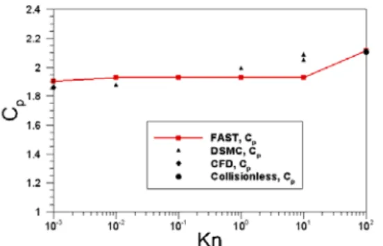
is compared with data from [9] on Figure 5. The pressure coefficient decrease from 2.1 to 1.9 from free-molecular regime to continuum regime respectively. In free-molecular regime, the exact value is obtained with FAST, whereas in continuum regime, a deviation of 2.6% is obtained with CFD. The maximal discrepancy (5.9%) is reached for Kn = 10. A satisfactory agreement is observed between DSMC data and FAST ones for the sphere. 2 0 1 s P P Cp − = 2 0s P f τ θ 2 ,stagsin p p C C = C =

(

)

Figure 6. Comparison between the pressure coefficient at stagnation point obtained with FAST and the data

from [9] for a sphere.

Aerodynamic forces and moments, and their corresponding coefficients, are computed by integration of pressure and friction coefficients on the object surface for different flow regimes (continuum, free-molecular and transitional).

4. AEROTHERMODYNAMICS MODELLING

In the case of vehicles and capsules, the equation controlling the temperature of the system is written taking into account the convective heat flux (qconv), the radiative heat flux from the shock layer (qrad,g) and the wall radiative cooling (qrad,w):

0 ) ( ) ( w + rad,g− rad,w w = convT q q T q (12)

The wall radiative cooling is given by the following equation, whatever the flow regime:

4

,w( w) w

rad T T

q =εσ (13)

where Tw is the wall temperature (K), ε the material emissivity and σ the Stefan-Boltzmann constant (W/m².K4).

4.1. Continuum flow

In the continuum flow domain, the convective heat flux at stagnation point can be computed by one of the following equations:

- Detra equation [10];

- Vérant-Lepage equation [11], [17]; - Vérant-Sagnier equation [12].

The Verant-Sagnier formulation is based on experimental measurements performed by [13] who have pointed out that the ratio qconvstag√(Rn/Pstag)/(Ht∞ -hw) is almost constant at stagnation point of a sphere for a wide range of freestream conditions and nose radius values.

The Verant-Sagnier [12] ONERA correlation used in FAST is written as following:

(14) 069 . 1 79 .

where Rn, is the nose radius (m) and

ref w t rT h H H = − Δ * ∞ . Htot is total enthalpy at free-stream conditions, hw is wall enthalpy, Tref = 273.15 K and r = 287 J/kg/K (air gas). It has to be noticed that the convective heat flux given by equation (14) assumes a fully catalytic wall.

The radiative heat flux at stagnation point coming from the radiative shock layer (qrad,g) can be computed with Tauber model [14] or with Martin model [15].

In continuum regime, the 3D heat flux distribution at the wall is computed from the reference heat flux at stagnation point thanks to Vérant-Lefrançois model [16], [17]:

(15) where R(x,y,z) is the local curvature radius (m), Rn is the nose curvature radius (m), P is the local pressure value (Pa). The reference heat flux value at stagnation point is given by:

g rad stag conv stag total stag ref q q q q = = + (16)

β power is determined using spheres as calibration cases whereas α is a function of local curvature radius which has been determined using numerical simulations database [18].

A most important point is that surfaces are assumed to behave as fully catalytic walls, which means that convective heat flux is going to be overestimated. Therefore, in the case of orbital debris, ground damage is going to be under-estimated.

In a model like harmonic oscillator (vibrational levels of molecules are excited) , wall enthalpy can be written as following: (17) θ0 = 3000 K w w w w w T Cp T T h ( )= ( ) (18)

The wall temperature Tw is obtained by solving the radiative equilibrium equation.

4.2. Free molecular and transitional flows

In the case of free molecular flow (Kn > 100), the Bird’s formula for the heat flux are used [7].

23 _⎜⎜⎛ − _⎟⎟⎞ = P H h q ⎠ ⎝ ∞ ref w t N stag conv stag rT R 8 . 0 , ( = ⋅ _⎟⎟⎞ _⎜⎜ _⎟ = ⎟ ⎝ β y R q y ( , , ) ) , , ( ) , , ) , , ( ⎟ ⎠ ⎞ ⎝ ⎛ ⎠ ⎜⎜ ⎝ ⎛ α⎜⎜⎛ ⎟_⎠⎞ β stag z y x R R N ref total P z x P z y x R z x q N 2 296 0 ⎞ ⎛ ⎟⎟ ⎠ ⎝ = Cp θ 2 0 1 1005 ) ( 0 ⎟ ⎟ ⎠ ⎜ ⎜ ⎝ − ⎞ ⎜⎜ ⎛ + w w T T w w w e e T T θ θ

Figure 6. Comparison of the heat flux coefficient obtained with FAST at stagnation point of a sphere with

data from literature [9].

In the transitional flow domain (10-3 < Kn < 100), the bridging function used is similar to the one presented above (Eq. 10 and 11); only the values of the coefficients n, a1, a2 have been modified.

The comparison of the stagnation point heat flux coefficient of a sphere obtained with FAST results with DSMC computations from [9] shows a good agreement between the two approaches (Figure 6).

5. APPLICATION TO SPACE VEHICLES 5.1. ARD vehicle

Atmospheric re-entry of the ARD vehicle (Figure 7) was the first European Union successful re-entry flight. Perfect gas and real gas Navier-Stokes computations have been performed by Walpot [19] using the ESA code LORE. Heat flux and pressure measurements along a body in wind tunnel have also been performed at the ONERA S4 wind tunnel and rebuilt by Walpot [19] using LORE computations. Flight points data used for LORE computations and S4 experimental conditions are given in Table 1. Computations and experiments have been conducted for 20° of angle of attack (α) and 0° of side slip angle (β).

Figure 7. ARD vehicle geometry [19].

Flight point Flight point Exp. S4 Exp. S4

M = 15 M = 24 P0 = 85 bar P0 = 25 bar Altitude [km] 51.53 65.83 Velocity [m/s] 4905.537 7212.43 1484 1454 Density [kg/m3] 9.211 x 10-41.5869 x 10-41.322 x 10-2 4.425 x 10-3 Temperature [K] 266.09 224.5 55.7 55.7 Pressure [Pa] 70.37 10.23 211.3 71.17 Units Case

Wall conditions 1500 K fixed

Fully catalytic

300 K fixed Fully catalytic

Table 1. Free-stream values and experimental conditions used for LORE computations and S4 wind

tunnel measurements, respectively.

Figure 8. Difference (in %) between the pressure distribution computed by FAST and LORE for M = 15.

The local pressure coefficient computed with FAST and LORE is compared in Figure 8 and Figure 9 for M = 15, α = 20° and β = 0°. A good agreement is observed, except in the elliptic flow region. Close to the shoulder, the information from the flow expansion goes back to the flow through the subsonic boundary layer. This is a characteristic problem of local method.

Figure 9. Comparison of pressure coefficient obtained with FAST and LORE in the ARD symmetry plane (y =

0) and for (M = 15; α = 20°, β = 0°).

The maximum heat flux computed with LORE and observed experimentally is not located at the stagnation point (stagnation pressure), but on the trailing edge, where the accelerated flow induces a decrease of the boundary layer, and thus, a strong increase of the temperature gradient and then heat flux. FAST under-estimates the heat flux obtained with LORE. However, Walpot [19] revealed the presence of a carbuncle phenomenon, influencing the shock capture. So, the LORE computation seems to over-estimate the peak of

heat flux (Figure 10) in the vicinity of trailing edge.

Figure 10.Comparison of LORE and FAST heat flux distribution in the ARD symmetry plane (y = 0) and for

(M = 15; α = 20°, β = 0°).

5.2. Pre-X (IXV-like vehicle)

Since the early 2000s, ONERA has been involved in experimental and numerical investigations performed to build the aerothermodynamic database for the IXV and Pre-X vehicles. Figure 11 exhibits Navier-Stokes chemical non-equilibrium computations of the flow around the Pre-X vehicle performed at two flight points using the ONERA CFD code CELHyO. Table 2 shows corresponding flight points data.

Figure 1. Navier-stokes computations for the Pre-X vehicle performed with the ONERA code CELHyO3D

for Mach 17.75 and Mach 25.

Mach [-] 17.75 25.0 Altitude [km] 62 73.6 Velocity [m/s] 5584 7205 Density [kg/m3] 2.579 x 10-4 5.546 x 10-5 Temperature [K] 245 207 Pressure [Pa] 18.22 3.11 rad. Equilibrium Fixed at

ε = 0.8 1500K Wall conditions

Table 2. Flight point data (PRE-X, phase A1), α = 40°, β = 0°, flaps deflection = 15°.

Those Navier-Stokes simulations, which are accurate but time-consuming, have been compared to FAST computations for the local pressure and heat flux

coefficients. Results obtained for Mach number 17.75 are shown in Figure 12 and Figure 13, respectively. Table 3 and Table 4 allow to perform a comparison of the pressure coefficient and heat flux at stagnation point for the two flight points considered (M = 17.75 and 25). A good agreement has been obtained at stagnation point for both flight points between FAST and Navier-Stokes computations.

Mach 17.75 25.0

Cp (CELHyO) 1.905 1.943

Cp (FAST) 1.925 1.943

Error (%) 1% 0%

Table 3. Comparison of pressure coefficient at stagnation point obtained with FAST and CELHyO3D.

M = 17.75 M = 25

qstag (CELHyO) W/m² 526 588

qstag (FAST) W/m² 519 536

Error (%) 1.3% 2%

Table 4. Comparison of convective heat flux at stagnation point obtained with CELHyO and FAST

(Vérant-Sagnier equation).

Figure 12. Comparison of pressure distribution obtained with FAST and CELHyO for PRE-X phase A1,

M = 17.75.

Figure 13. Comparison of heat flux distribution obtained with FAST (Vérant-Sagnier equation) and

Figure 12 and Figure 13 confirm that both pressure coefficient and heat flux values are matched pretty well all over the large blunted region of the vehicle. In the centre part of the windward side and upstream of the separation zone, differences lower than 15 % are still obtained for the heat flux value which is an acceptable number. However, strong discrepancies appear in the transverse flow regions, near the separation zone and on the flaps. It has to be noticed that errors from the modified Newton method have impacted the heat flux computation since the local pressure value is then used. In the particular case of the flaps, both shock-boundary layer interaction and separation modelling would require much higher level representation.

5.3. CubeSat (debris-like object)

In the frame of the QB50 project, ISAE and ONERA have been equipping a CubeSat dedicated to in-flight measurements characteristic of the atmospheric re-entry of an orbital debris single shape.

A smooth configuration for the cubesat has been computed using FAST and compared to non equilibrium flow simulations using the Navier-Stokes code CEDRE (ONERA).

Since many faces of the cubesat are flat plates, the cubesat has been divided in several domains :

- The heat flux value on flat plates is computed with FAST using effective nose radius as a function of the bluntness parameters.

- The heat flux value on other surfaces is computed using Eq. (14) and (15).

Figure 14. ISAE-ONERA cubesat “EntrySat” for the QB50 project

The flight point z = 70 km and V = 6692 m/s has been under investigation since this is a critical altitude for the cubesat which is to be destroyed before.

Navier-Stokes results are pictured on Figures 15 & 16. FAST computation of the surface heat flux is shown in Figure 17.

A good agreement has been found for the exposed face of the cubesat but the heat flux value is underestimated

at corners and trailing edges. Since the connexion between elements of a satellite can be a junction exposed to high heat flux levels (characteristic of a trailing edge), engineering methods should aim to improve heat flux prediction in such regions in future work.

Figure 15. Navier-Stokes computation of the Mach number using CEDRE

Figure 16. Navier-Stokes computation of the surface heat flux using CEDRE (W/cm²)

Figure 17. Navier-Stokes computation of the surface heat flux using FAST (W/cm²)

6. PERSPECTIVES

It is well known that modified Newtonian method is not suitable for many cases such as elliptic flows, high angle sphere-cones or deflected flaps. In the case of elliptic flows, a global method has been tested.

The principle and the used variables are defined on Figure. The shock curvature is assumed to be known. Many approximations based on the curvature radius value can be found [6], here an equation from Love et al. [18] has been used in the case of the AOTV vehicle. The object is assumed to be approximately 2D axisymmetrical. The global mass conservation through the control volume pictured on Figure 19 can be written as following: r r V dy r y u s y 2 1 ) cos( 2 0 ∞ ∞ = = ⎟ ⎠ ⎞ ⎜ ⎝ ⎛ ₊

∫

Assuming that ρu is constant along the section 4, it comes: ρ θ δ δ ρ )) cos( 2 ( 2 2 + = ∞ ∞ r r V u s

Pressure is then obtained by isentropic expansion from stagnation point : 1 2 1 1 1 2 1 1 − − ⎟ ⎠ ⎞ ⎜ ⎝ ⎛ ₊ − = γ γ γ u stag M P P u u a u M = , 12 2 1 2 2 1 ,a au u − + = γ

with Mu = u/a and a12 = au2 + (γ1 - 1)/2×u2

Figure 18. AOTV vehicle

Figure 19. Global method for 2D flows.

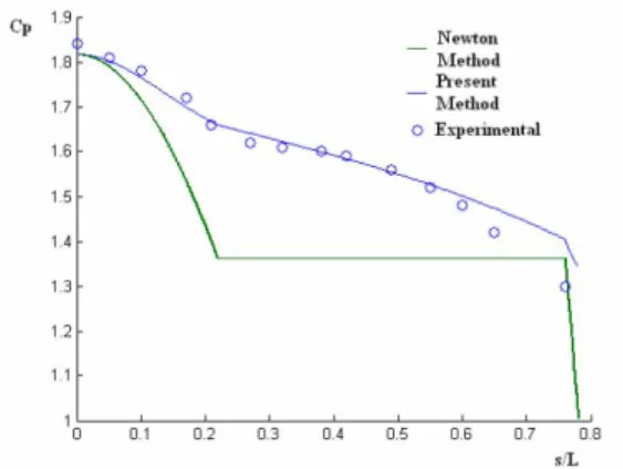
On figure 20 and 21, the results are compared to experimental measurements performed by Wells et al. [20].

A significant improvement can be observed compared to the modified Newton method. However, Figures 6 and 7 show that the method is sensitive to the shock curve location accuracy.

Although that global approach has not been generalized to any 3D flow yet, it can use all other developments performed in FAST.

Figure 20. Global method for pressure determination (AOTV vehicle). A Love’s formulation has been used for

the shock curve location.

Figure 21. Global method for pressure determination (AOTV vehicle). A 2D Navier-stokes computation has

been used for the shock curve location.

7. CONCLUSIONS

The main aerothermodynamics models implemented in the ONERA FAST code have been described. An original feature is that geometrical components of the object are not separately processed but they are investigated by a global method taking into account

geometrical effects and flow history for the wall heat flux distribution prediction.

A major advantage is that the approach remains low time-consuming compared to Navier-Stokes simulations and it can easily be coupled to a computational dynamic flight . The modelling developed for FAST allows computing a complete trajectory from its entry point since continuum, free molecular and transitional flow have been addressed.

Comparisons have been performed on a list of vehicles (but representatives of atmospheric re-entry activities in European Union) that have pointed out some weak and strong points in the present modelling.

Elliptic flow regions, mainly encountered by capsules thermal shields or manoeuvring surfaces like flaps, cannot be correctly described by a Newtonian approach but it has been shown that results could be significantly improved by using non-local methods. The difficulty relies on their implementation for any investigated 3D objects.

It has also been noticed that boundary layer thickness could play a significant role for local heat flux assessment at trailing edges for instance. Therefore a boundary layer modelling might be considered to address such issue.

A prime important point concerning application to orbital debris risk assessment is the development of corrected laws taking account of partial catalycity at wall according to non metallic materials. Otherwise the heat fluxes values should be overestimated as the addressed risk at ground. Specific features such as tumbling of the object (unsteady heat flux process), strong curvature radius variations (due to the object design, tumbling, wall ablation) require additional modelling for aerothermodynamics. Multi-physics phenomena such as heat transfer inside the object (conduction [6] [17], radiation, pyrolysis), breaking up, possible interaction between fragments [6], [21] require specific developments as well.

References

1. Laroche, E., Prévereaud, Y., Vérant, J-L., Sourgen, F., Bonetti, D. (2015). Aerothermodynamics analysis of the Spaceliner Cabin Escape System modified via a morphing system. 8th Europ. Symp.

Aerothermodyn. Space Veh., to be published, 2-6th

march 2015, Lisbon, Portugal.

2. Jouhaud, F. (2011). Atmospheric and Space Flight Mechanics: collection of models, Technical Rapport NT 4/17163 DCSD, ONERA (in French). 3. Diallo, A. (2005). Automatic Surface Heating

Description in Hypersonic Continuum Regime. Master Thesis, ISAE and Politecnico di Torino. 4. Srinivasan, S., Tannehill, J.C. & Weilmuenster, K.J.

(1987). Simplified Curve Fits for the

Thermodynamic Properties of Equilibrium Air, Tech. Rep. NASA-RP-1181.

5. Bertin, J.J. (1938). Hypersonic Aerothermodynamics. AIAA Education Series.

6. Prévereaud, Y. (2014). Development of models for the atmospheric re-entry of space debris, Ph.D. Thesis, Toulouse University, Toulouse, France (in French).

7. Bird, G.A. (1994). Molecular Gas Dynamics and the

Direct Simulation of Gas Flows. Oxford Science

Publications, Oxford Engineering Scienc Series number 42.

8.Blanchard, R.C. (1991). Rarefied-Flow Aerodynamics Measurement Experiment on the Aeroassist Flight Experiment Vehicle. J. Space. Rockets 28 (4), 368-375.

9. Glass, C.E., Moss, J.N. (2001). Aerothermodynamic Characteristics in the hypersonic Continuum-Rarefied transitional Regime. 35th AIAA thermophys. Conf. Anaheim, USA.

10. Detra, R.W., Kemp, N.H. & Riddell, F.R. (1957). Addendum to 'Heat Transfer to Satellite Vehicle Re-entering the Atmosphere', Jet Prop. 27 (12), 1256-1257.

11. Lepage, Y. (2005). Correlation du flux de chaleur convectif au point d’arrêt lors d’une rentrée atmospherique terrestre. Master Thesis, Ecole Polytecnique, Paris (In French).

12. Sagnier, P. & Vérant, J-L. (1998). Flow Characterization in the ONERA F4 high enthalpy wind tunnel, AIAA J. 36 (4), 522-531.

13. Sutton, K. & Graves, R.A. (1971). A general stagnation point convective heating equation for arbitrary gas mixtures. NASA Technical report TR-376.

14. Tauber, M.E. & Sutton, K. (1991). Stagnation-Point Radiative Heating Relations for Earth and Mars Entries, J. Space. Rockets 28 (1), 40-42.

15. Martin, J.J. (1966). Atmospheric Reentry, an

introduction to its science and engineering.

Prentice-Hall international series in space technology.

16. Lefrançois, R. (2006). Calcul avant-projet du flux de chaleur lors d’une rentrée atmosphérique. Projet d’Initiation à la Recherche, ISAE, Toulouse. 17. Prevereaud, Y. Vérant, J-L. & Balat-Pichelin, M.

(2014). Orbital Debris Atmospheric Re-entry Prediction. In Proc. 65th International Astronautical Congress, IAC-14-A6.9.10, Toronto, Canada (submitted for publication).

Moschetta, J-M., Manuel mathematique, ONERA report RF 1/20874, Dec. 2012 (in french)

19. Walpot, L. (2002). Development and Application of Hypersonic Flow Solver. Ph.D Thesis. Deft Technical University, The Netherlands.

20. Wells, William L., Measured and Predicted Aerodynamic Coefficients and Shock Shapes for Aeroassist Flight Experiment Configuration, NASA TP-2956, 1990

21. Prévereaud, Y., Vérant, J-L., Moschetta, J-M., Sourgen, F. (2013). Debris Aerodynamic interaction and its Effect on re-entry risk Assessment. 6th Europ. Conf. Space Debris, Darmstadt, Germany.