HAL Id: hal-00307791
https://hal.archives-ouvertes.fr/hal-00307791
Submitted on 15 Sep 2009
HAL is a multi-disciplinary open access
archive for the deposit and dissemination of
sci-entific research documents, whether they are
pub-lished or not. The documents may come from
teaching and research institutions in France or
abroad, or from public or private research centers.
L’archive ouverte pluridisciplinaire HAL, est
destinée au dépôt et à la diffusion de documents
scientifiques de niveau recherche, publiés ou non,
émanant des établissements d’enseignement et de
recherche français ou étrangers, des laboratoires
publics ou privés.
L(p,q) labeling of d-Dimensional Grids
Guillaume Fertin, André Raspaud
To cite this version:
Guillaume Fertin, André Raspaud. L(p,q) labeling of d-Dimensional Grids. Discrete Mathematics,
Elsevier, 2007, 307 (16), pp.2132-2140. �hal-00307791�
L
(p, q) Labeling of d-Dimensional Grids
∗
Guillaume Fertin
1, Andr´
e Raspaud
21LINA FRE CNRS 2729, Universit´e de Nantes
2 rue de la Houssini`ere - BP 92208 - F44322 Nantes Cedex 3
2LaBRI UMR 5800, Universit´e Bordeaux 1
351 Cours de la Lib´eration - F33405 Talence Cedex
[email protected], [email protected]
Abstract
In this paper, we address the problem of λ labelings, that was introduced in the context of frequency assignment for telecommunication networks. In this model, stations within a given radius r must use frequencies that differ at least by a value p, while stations that are within a larger radius r0 > rmust use frequencies that differ by at least another value q. The aim
is to minimize the span of frequencies used in the network. This can be modeled by a graph coloring problem, called the L(p, q) labeling, where one wants to label vertices of the graph Gmodeling the network by integers in the range [0; M ], in such a way that (1) neighbors in Gare assigned colors differing by at least p and (2) vertices at distance 2 in G are assigned colors differing by at least q, while minimizing the value of M . M is then called the λ number of G, and is denoted by λp
q(G).
In this paper, we study the L(p, q) labeling for a specific class of networks, namely the d-dimensional grid Gd= G[n1, n2. . . nd]. We give bounds on the value of the λ number of an
L(p, q) labeling for any d ≥ 1 and p, q ≥ 0. Some of these results are optimal (namely, in the following cases : (1) p = 0, (2) q = 0, (3) q = 1 (4) p, q ≥ 1, p = α · q with 1 ≤ α ≤ 2d and (5) p ≥ 2dq + 1) ; when the results we obtain are not optimal, we observe that the bounds differ by an additive factor never exceeding 2q − 2. The optimal result we obtain in the case q= 1 answers an open problem stated by Dubhashi et al. [DMP+02], and generalizes results
from [BPT00] and [DMP+
02]. We also apply our results to get upper bounds for the L(p, q) labeling of d-dimensional hypercubes.
1
Introduction
In this paper, we study the frequency assignment problem, originally introduced in [Hal80], where radio transmitters that are geographically close may interfere if they are assigned close frequencies. This problem arises in mobile or wireless networks. Generally, this problem is modeled by a graph coloring problem, where the transmitters are the vertices, and an edge joins two transmitters that are sufficiently close to potentially interfere. The aim here is to color (i.e. give an integer value, corresponding to the frequency) the vertices of the graph in such a way that :
• any two neighbors (transmitters that are very close) are assigned colors (frequencies) that differ by a parameter at least p ;
• any two vertices at distance 2 (transmitters that are close) are assigned colors (frequencies) that differ by a parameter at least q ;
∗Part of this work was done while both authors were visiting the Universitat Polit`ecnica de Catalunya in
• the greatest value for the colors is minimized.
It has been proved that under this model, we could assume the colors to be integers, start-ing from 0 [GY92]. In that case, the minimum range of frequencies that is necessary to assign the vertices of a graph G is denoted λp
q(G), and the problem itself is usually called the L(p, q)
labeling problem. The frequency assignment problem has been studied in many different specific topologies [GY92, Sak94, WGM95, BPT00, BKTvL00, CKK+02, MS02, BPT02, Kra, FKP01]. The case p = 2 and q = 1 is the most widely studied (see for instance [CK96, JNS+00, Jha00, CP01, FKK01]). Some variants of the model also exist, such as the following generalization, called the L(δ1, . . . δk) labeling problem, where one gives k constraints on the k first distances (any two
vertices at distance 1 ≤ i ≤ k in G must be assigned colors differing by at least δi). One of
the issues also considered in the frequency assignment problem is the no-hole property, where one wants to know whether a given coloring with span M uses all the possible colors in the range [0; M ].
In this paper, we focus on the L(p, q) labeling problem, and we study in Section 2 the case of the L(p, q) labeling in the d-dimensional grid Gd. We first address in Section 2.1 the cases where
p= 0 or q = 0. In Section 2.2, we give results for the L(p, q) labeling of Gd for any p, q, d ≥ 1.
We give lower and upper bounds on λp
q(Gd), and show that in some cases, these bounds coincide.
Notably, in the case q = 1, the results we obtain are optimal ; this answers an open problem stated by Dubhashi et al. in [DMP+02], and generalizes results from [BPT00] and [DMP+02].
The results we give are also optimal when p = 0, q = 0, p = α · q with 1 ≤ α ≤ 2d, and p ≥ 2dq + 1. We prove that in some cases (namely, when 1 ≤ p ≤ 2dq), one of the colorings we propose satisfies the no-hole property. We also apply our results to get upper bounds for the L(p, q) labeling of d-dimensional hypercubes.
2
L
(p, q) labeling of G
dWe now turn to the case of the λ labeling problem with two constraints on the distances, in a particular network topology, namely the d-dimensional grid Gd = G[n1, n2. . . nd]. We first recall
the definition of such a network.
Definition 1 Let d ∈ N and (n1, . . . , nd) ∈ Nd, with ni≥ 2 for any 1 ≤ i ≤ d. The d−dimensional
grid of lengths n1, . . . , nd, denoted by Gd(n1, . . . , nd), is the following graph:
V(Gd(n1, . . . , nd)) = [1, n1] × [1, n2] × · · · × [1, nd]
E(Gd(n1, . . . , nd)) = {{u, v} | u = (u1, . . . , ud), v = (v1, . . . , vd), and there exists i0 such that
∀i 6= i0, ui= vi, and |ui0− vi0| = 1}
We first address the L(p, q) labeling of Gd in the special cases where p = 0 (resp. q = 0) in
Section 2.1. We then address the more general case where p, q ≥ 1 in Section 2.2.
2.1
L
(p, q) labeling when p = 0 or q = 0
Proposition 1 For any p ≥ 0 and d ≥ 1, λp0(Gd) = p.
Proof : Consider an optimal L(p, 0) labeling of the vertices of Gd. Clearly, there must exist a
vertex, say v, with color c(v) = 0 (if not, then λp0(Gd) could be reduced by at least 1). Then, any
neighbor of v must have a color greater than or equal to p. Thus, λp0(Gd) ≥ p.
Now, since Gdis bipartite, we have that λ p
0(Gd) ≤ p. Indeed, let us define the following coloring:
for any vertex v = (x1, x2. . . xd), ifP d
i=1xi ≡ 0 mod 2, then c(v) = 0, otherwise c(v) = p. Since
q= 0, it suffices to check that any two neighbors are assigned colors that differ by at least p. It is clearly the case here, since any two neighbors in Gd have the sum of their coordinates of different
parity, and thus will be assigned different colors. Since the colors are taken in the set {0, p}, we have that any two neighbors u and v in Gd satisfy |c(u) − c(v)| ≥ p. Hence we have λ
p
0(Gd) = p.
Proposition 2 For any q ≥ 0 and d ≥ 1, λ0
q(Gd) = (2d − 1)q.
Proof : Consider a vertex v of degree 2d in Gd, and let c(v) be its color in an optimal L(0, q)
labeling of Gd. In that case, at most one neighbor of v, say w, can satisfy c(v) = c(w). Thus,
there remains 2d − 1 neighbors of u to color, and since those vertices are at distance 2 from w and from each other, they must use colors that are pairwise q away. Thus, if we assume w.l.o.g. c(v) = c(w) = 0, then the best we can expect for those 2d − 1 vertices is that they be assigned colors in the set q, 2q . . . (2d − 1)q. Hence, λ0
q(Gd) ≥ (2d − 1)q.
Now we give an L(0, q) labeling of Gd that uses colors in the set {0, p, 2q . . . (2d − 1)q} : for
any vertex v = (x1, x2. . . xd) of Gd, we define
c(v) = (dqbxd 2 c + d−1 X i=1 iqxi) mod 2dq
Since p = 0, we only need to consider two vertices u and v lying at distance 2 in Gd, thus differing
on two coordinates, say xi and xj, 1 ≤ i ≤ j ≤ d. W.l.o.g. we can consider only two cases,
supposing u = (x1, . . . xi. . . xj. . . xd) : (1) v = (x1, . . . xi+ 1 . . . xj + 1 . . . xd) (where possibly
i= j) and (2) v = (x1, . . . xi+ 1 . . . xj− 1 . . . xd) (where i 6= j). In case (1), we will distinguish
two cases : (1a) i = j and (1b) i 6= j. In case (1a), we have again two cases two consider : first, if i= j = d, then clearly |c(v) − c(u)| = dq, and the condition is satisfied since d ≥ 1. If i = j 6= d, then |c(v) − c(u)| = 2iq, since 1 ≤ i ≤ d − 1. Thus the condition is satisfied as well. Now we turn to case (1b), where i 6= j. W.l.o.g., we thus consider 1 ≤ i < j ≤ d. If j = d, then depending on the parity of xd, we either obtain |c(v) − c(u)| = iq (for even xd) or |c(v) − c(u)| = (i + d)q (for
odd xd). In both cases, since i ≤ d − 1, we see that the condition is satisfied. Now, if j 6= d, then
|c(v) − c(u)| = (i + j)q, which also satisfies the condition that the colors differ by at least q. In case (2), we know that necessarily i 6= j, and thus we consider as above 1 ≤ i < j ≤ d. First, if j = d, then depending on the parity of xd, we either obtain |c(v) − c(u)| = iq (for even xd) or
|c(v) − c(u)| = (d − i)q (for odd xd). In both cases, the condition is satisfied since 1 ≤ i ≤ d − 1.
Now, if j 6= d, we get |c(v)−c(u)| = (j −i)q, which also satisfies the conditions since 1 ≤ i < j ≤ d. Overall, we see that this coloring satisfies the distance 2 condition, and thus is valid to L(0, q) label Gd. Since it uses colors in the set {0, q, 2q, . . . (2d−1)q}, we conclude that λ0q(Gd) ≤ (2d−1)q.
Hence, altogether we have λ0
q(Gd) = (2d − 1)q. 2
We note that except in specific cases, the colorings we have given above do not satisfy the no-hole property (we recall that the no-hole property holds when all colors in the range [0; λp
q] are
used). Indeed, in the case q = 0, only colors 0 and p are used, thus the coloring is not no-hole for any p ≥ 2. Similarly, in the case p = 0, the colors used are taken in the set {0, q, 2q . . . (2d − 1)q}, thus the coloring is not no-hole for any q ≥ 2.
2.2
L
(p, q) labeling when p, q ≥ 1
We now address the L(p, q) labeling of Gd, for any values of p, q ≥ 1 and d ≥ 1. First, we note
that we can obtain two trivial upper bounds on λp
q(Gd) ; this is described in the two following
observations.
Observation 1 For any p, q, d ≥ 1, λp
q(Gd) ≤ q · λ dp
qe 1 (Gd).
Proof : The key idea here is to first achieve an L(α, 1) coloring C of Gd (thus with λ number
λα
1(Gd)), and to get another coloring C0by multiplying the color of each vertex by q. In that case,
two vertices at distance 2 in Gd, which were assigned different colors by C, are assigned colors
differing by at least q in C0. Moreover, two neighbors in G
d are now assigned colors differing by
at least αq. Since we want αq ≥ p, it suffices to take α = dpqe. 2
There exists another upper bound for λp
q(Gd), that relies on the L(1, 1) labeling of Gd. We
Observation 2 For any p, q, d ≥ 1, λp
q(Gd) ≤ max{p, q} · 2d.
Proof : Let C denote the coloring derived from an optimal L(1, 1) of Gd, and let C0 be a new
coloring obtained from C by multiplying every color by max{p, q}. In that case, any two vertices at distance 1 (resp. 2) in Gdare assigned colors that are at least p (resp. at least q) apart. Hence
this is an L(p, q) labeling of Gd. Since we know (cf. for instance [FGR03] or Theorem 1 below)
that λ1
1(Gd) = 2d, we conclude that λpq(Gd) ≤ max{p, q} · 2d. 2
The two above mentioned simple observations present the disadvantage to be based upon an existing labeling (an L(p, 1) labeling for Observation 1, and an L(1, 1) labeling for Observation 2). In the following, we study the problem in more details, and define upper and lower bounds on λp
q(Gd) for all values of p, q, d ≥ 1 (resp. in Lemmas 1 and 2). These results directly imply
Theorem 1.
Lemma 1 For any p, q, d ≥ 1, • λp
q(Gd) ≥ 2p + (2d − 2)q when 1 ≤ p ≤ 2dq
• λp
q(Gd) ≥ p + (4d − 2)q when p ≥ 2dq + 1
Proof : Suppose that it is possible to L(p, q) label the vertices of Gd with M colors, with M ≤
2p + (2d − 2)q − 1. We will first show that in that case, no vertex of degree 2d in Gd can be
assigned a color in the range [p − 1; p + (2d − 1)q − 1].
Indeed, suppose there exists a vertex u ∈ V (Gd) such that u is assigned color p + x, with −1 ≤
x≤ (2d − 1)q − 1. Then, all its neighbors must be assigned a color in the range [0; x] ∪ [2p + x; M ], because of the gap of at least p that must exist between neighbors. Within this range, one must be able to get 2d values, each pair of which differ of at least q. Let us distinguish two cases : (i) x= −1 and (ii) x ≥ 0. In case (i), it is clear that all the colors must be in the range [2p − 1; M ]. In other words, if we want to be able to assign the 2d colors of the neighbors, we must have 2p − 1 + (2d − 1)q ≤ M . However, we supposed M ≤ 2p + (2d − 2)q − 1, hence the contradiction since q ≥ 1. Now suppose that (ii) x ≥ 0 ; we distinguish two more cases : (ii-1) x = kq with k≥ 0 and (ii-2) x = kq − i, with k ≥ 1 and 1 ≤ i ≤ q − 1. In case (ii-1), we can use (k + 1) colors in the range [0; kq] (more precisely, colors 0, q, 2q . . . kq). Hence there remains 2d − (k − 1) colors to get in the range [2p + x; M ]. For this, we must have 2p + x + (2d − (k − 1) − 1)q ≤ M . This gives 2p + (2d − 2)q ≤ M , a contradiction. In case (ii-2), only k colors can be assigned in the range [0; x]. Thus 2d − k colors must be assigned in the range [2p + x; M ], which can be the case only if 2p + x + (2d − k − 1)q ≤ M . This can happen only when i ≥ q + 1, a contradiction too. Thus we conclude that if λp
q(Gd) = M , no vertex of degree 2d in Gd can be assigned a color in the range
[p − 1; p + (2d − 1)q − 1].
In other words, if such a coloring exists, all vertices of degree 2d are assigned colors in the range [0; p−2]∪[p+(2d−1)q; M ]. Let I1= [0; p−2] and I2= [p+(2d−1)q; M ], with M = 2p+(2d−2)q−j,
j≥ 1. Clearly, I1contains p − 1 integers, and I2contains p − q − j + 1 < p integers (since j, q ≥ 1).
This means that if a vertex u of degree 2d in Gdis assigned a color in I1(resp. I2), all its neighbors
must be assigned colors in I2 (resp. I1) – supposing that all the neighbors of u are of degree 2d,
which happens if Gd is “big” enough. However, in order for I1 (resp. I2) to support 2d colors
that, pairwise, admit a gap of q, the two following conditions must be fulfilled : (1) (2d − 1)q ≤ p − 2 and
(2) p + (2d − 1)q + (2d − 1)q ≤ M
In other words, we must have (1’) p ≥ (2d − 1)q + 2 and (2’) p ≥ 2dq + j. Since j, q ≥ 1, condi-tion (2’) implies condicondi-tion (1’). Thus, in order to have a valid L(p, q) labeling with λp
q(Gd) = M ,
we must have p ≥ 2dq + j with j ≥ 1. However, we supposed p ≤ 2dq, hence the contradiction. Overall, we have proved that for a sufficiently large grid, and when 1 ≤ p ≤ 2dq, λp
q(Gd) ≥
Now suppose that p ≥ 2dq + 1. Suppose that λp
q(Gd) = M0, with M0 < p+ (4d − 2)q. Since
we supposed that p ≥ 2dq + 1, we have p + (4d − 2)q < 2p + (2d − 2)q, we can reuse one of the previous arguments and conclude that no vertex of degree 2d can be assigned a color in the range [p − 1; p + (2d − 1)q − 1]. Hence all the vertices of degree 2d must be assigned colors in [0; p − 2] ∪ [p + (2d − 1)q; M0]. We also use one of the previous arguments here to say that in
that case we must have (1) (2d − 1)q ≤ p − 2 and (2) p + (2d − 1)q ≤ M0. However, (2) is not
satisfied, hence the contradiction. We then conclude that necessarily, in the case p ≥ 2dq + 1, λp
q(Gd) ≥ p + (4d − 2)q. 2
Lemma 2 For any p, q, d ≥ 1, • λp q(Gd) ≤ 2dq when 2 ≤ 2p < q • λp q(Gd) ≤ 2p + (2d − 1)q − 1 when 1 ≤ q ≤ 2p ≤ 4dq • λp q(Gd) ≤ p + (4d − 2)q when p ≥ 2dq + 1
Proof : Let p, q, d ≥ 1. In order to prove these upper bounds, we give an ad hoc coloring in each of the two cases, and show that it respects the constraints at distances 1 and 2.
Case 1: 2 ≤ 2p < q. For any vertex v = (x1. . . xd) in Gd, with xi ≥ 0 for any 1 ≤ i ≤ d,
we assign to v color c(v) defined as follows :
c(v) = (
d
X
i=1
qixi) mod (2d + 1)q
We are going to prove that this coloring is an L(p, q) labeling of Gd. For this, we distinguish
two cases :
• u and v are neighbors in Gd, thus they differ on one coordinate xi, 1 ≤ i ≤ d. W.l.o.g.,
suppose u = (x1, . . . xi. . . xd) and v = (x1, . . . xi+ 1 . . . xd). In that case |c(v) − c(u)| = iq
mod (2d + 1)q. Since 1 ≤ i ≤ d, we have that |c(v) − c(u)| ≥ q. However, we supposed p <2q, thus we conclude q > p and |c(v) − c(u)| > p.
• u and v lie at distance 2 in Gd, thus they differ on two coordinates xiand xj, 1 ≤ i ≤ j ≤ d.
W.l.o.g. we can consider only two cases, supposing u = (x1, . . . xi. . . xj. . . xd) : (1) v =
(x1, . . . xi+1 . . . xj+1 . . . xd) (where possibly i = j) and (2) v = (x1, . . . xi+1 . . . xj−1 . . . xd)
(where i 6= j). In case (1) we have |c(v) − c(u)| = (i + j)q mod (2d + 1)q. Since 1 ≤ i, j ≤ d, we conclude that |c(v) − c(u)| ≥ 2q, and thus |c(v) − c(u)| ≥ q. In case (2), we have |c(v) − c(u)| = (j − i)q mod (2d + 1)q. Since 1 ≤ i < j ≤ d (because we supposed that j ≥ i, and since we are in case (2), i 6= j), we have that |c(v) − c(u)| ≥ q. Hence the constraint is satisfied in both cases.
Hence, the above mentioned coloring is an L(p, q) labeling of the grid in the case p, q, d ≥ 1 and 2p < q. Since it uses colors in the set {0, q, 2q, . . . 2dq}, we conclude that λp
q(Gd) ≤ 2dq.
Case 2: 1 ≤ q ≤ 2p ≤ 4dq. For any vertex v = (x1. . . xd) in Gd, with xi ≥ 0 for any 1 ≤ i ≤ d,
we assign to v color c(v) defined as follows :
c(v) = (
d
X
i=1
(p + (i − 1) · q)xi) mod (2p + (2d − 1)q)
We are going to prove that this coloring is an L(p, q) labeling of Gd. For this, we distinguish
• u and v are neighbors in Gd, thus they differ on one coordinate xi, 1 ≤ i ≤ d. W.l.o.g.,
suppose u = (x1, . . . xi. . . xd) and v = (x1, . . . xi+1 . . . xd). Thus |c(v)−c(u)| = (p+(i−1)q).
Since 1 ≤ i ≤ d, we have that |c(v) − c(u)| ≥ p.
• u and v lie at distance 2 in Gd, thus they differ on two coordinates xiand xj, 1 ≤ i ≤ j ≤ d.
W.l.o.g. we can consider only two cases, supposing u = (x1, . . . xi. . . xj. . . xd) : (1) v =
(x1, . . . xi+1 . . . xj+1 . . . xd) (where possibly i = j) and (2) v = (x1, . . . xi+1 . . . xj−1 . . . xd)
(where i 6= j). In case (1), |c(u) − c(v)| = 2p + (i + j − 2)q. In that case, |c(u) − c(v)| ≥ q, except maybe when i = j = 1. However, when i = j = 1, then |c(u) − c(v)| = 2p, and by hypothesis we know that 2p ≥ q. Thus |c(u) − c(v)| ≥ q in all the cases. In case (2), since i6= j, we have that j > i. Then we have |c(u) − c(v)| = (j − i)q. Thus, for any two vertices u, v∈ V (Gd) that lie at distance 2, we have |c(u) − c(v)| ≥ q.
Hence, we have proved that the above mentioned coloring is an L(p, q) labeling of the grid in the case p, q, d ≥ 1, 1 ≤ q ≤ 2p ≤ 4dq. Since it uses colors in the range [0; 2p + (2d − 1)q − 1], we conclude that λp
q(Gd) ≤ 2p + (2d − 1)q − 1.
Case 3: p ≥ 2dq + 1. In this case, any vertex having an even sum of coordinates will be as-signed a color in the range [p + (2d − 1)q; p + (4d − 2)q], while any vertex having an odd sum of coordinates will be assigned a color in the range [0; (2d − 1)q]. More precisely, for any vertex v= (x1. . . xd) in Gd, with xi≥ 0 for any 1 ≤ i ≤ d, we assign to v color c(v) defined as follows :
(1) for any v such thatPdi=1xi≡ 0 mod 2,
c(v) = [(1 2 d X i=1 (2i − 1)qxi) mod (2d − 1)q + 1] + (p + (2d − 1)q)
(2) for any v such thatPdi=1xi≡ 1 mod 2,
c(v) = [(1 2[
d
X
i=1
(2i − 1)qxi− odd(q)]) mod (2d − 1)q + 1
In order to prove that this is an L(p, q) labeling of Gd, let us consider the two following cases :
• u and v are neighbors in Gd, thus they differ by one on exactly one coordinate xi, 1 ≤ i ≤ d.
Let u = (x1, . . . xi. . . xd) and v = (y1, . . . yi. . . yd), S(u) =Pdi=1xiand S(v) =Pdi=1yi. We
clearly see that if S(u) is even, then S(v) is odd and vice-versa. Since in the case where S(u) is even (resp. odd), c(u) ∈ [p + (2d − 1)q; p + (4d − 2)q] (resp. c(u) ∈ [0; (2d − 1)q]), we conclude that in all the cases, |c(v) − c(u)| ≥ p.
• Suppose now that u and v lie at distance 2 in Gd : thus u and v differ on two coordinates
xi and xj, 1 ≤ i ≤ j ≤ d. W.l.o.g. we can consider only two cases, supposing u =
(x1, . . . xi. . . xd) : (a) v = (x1, . . . xi+ 1 . . . xj+ 1 . . . xd) (where possibly i = j) and (b)
v = (x1, . . . xi+ 1 . . . xj− 1 . . . xd) (where i 6= j). We also know that S(u) and S(v) have
same parity. Thus for each of the cases (a) and (b), there are 2 cases to consider : (a-even) (resp. (b-even)) in case (a) (resp. (b)) when S(u) and S(v) are even and (a-odd) (resp. (b-odd)) in case (a) (resp. (b)) when S(u) and S(v) are odd. We detail each of those 4 cases below.
– (a-even) : |c(v) − c(u)| = 1
2((2i − 1)q + (2j − 1)q), that is |c(v) − c(u)| = (i + j − 1)q.
Hence, c(u) and c(v) differ by at least q, since 1 ≤ i, j ≤ d.
– (b-even) : Since i 6= j let us suppose w.l.o.g. that 1 ≤ i < j ≤ d. Hence |c(u) − c(v)| =
1
2((2j − 1)q − (2i − 1)q), that is |c(u) − c(v)| = (j − i)q. Since 1 ≤ i < j ≤ d, c(u) and
– (a-odd) : |c(v) − c(u)| = 1
2((2i − 1)q + (2j − 1)q), that is |c(v) − c(u)| = (i + j − 1)q.
But since 1 ≤ i ≤ j ≤ d, we conclude that c(u) and c(v) differ by at least q.
– (b-odd) : Since i 6= j let us suppose w.l.o.g. that 1 ≤ i < j ≤ d. Hence |c(u) − c(v)| =
1
2((2j − 1)q − (2i − 1)q), that is |c(u) − c(v)| = (j − i)q. But since 1 ≤ i < j ≤ d, we
conclude that c(u) and c(v) differ by at least q.
Hence, we have proved that the above mentioned coloring is an L(p, q) labeling of the grid in the case p, q, d ≥ 1 with p ≤ 2dq + 1. Since it uses colors in the range [0; (2d − 1)q] ∪ [p + (2d − 1)q; p + (4d − 2)q], we conclude that λp
q(Gd) ≤ p + (4d − 2)q. Altogether, this proves the lemma. 2
As a consequence of Lemmas 1 and 2, we have the following theorem.
Theorem 1 (L(p, q) labeling of d-dimensional Grids, for any value of p, q, d ≥ 1) Let p ≥ 1 and d ≥ 1. Then : • 2p + (2d − 2)q ≤ λp q(Gd) ≤ 2dq when 2 ≤ 2p < q • 2p + (2d − 2)q ≤ λp q(Gd) ≤ 2p + (2d − 1)q − 1 when 1 ≤ q ≤ 2p ≤ 4dq • λp q(Gd) = p + (4d − 2)q when p ≥ 2dq + 1
When 1 ≤ q ≤ 2p ≤ 4dq, the bounds we get coincide in the case q = 1, thus yielding an optimal L(p, 1) labeling of Gd. We note that this generalizes Lemma 5 of [BPT00] and Theorem 3
of [DMP+02], and also answers an open problem stated in [DMP+02].
By combining some of the previous results, it is possible to improve some of the upper bounds obtained above. More precisely, this is done thanks to a combination of the results from Observa-tion 1 and Theorem 1. This is the purpose of the following proposiObserva-tion.
Proposition 3 For any d ≥ 1 :
• for any q ≥ 1, and any p = αq with 1 ≤ α ≤ 2d, λp
q(Gd) = 2p + (2d − 2)q
• for any q ≥ 1 and any p = αq + β with 1 ≤ β ≤ q − 1 and p ≤ 2dq + β − q, λp q(Gd) ≤
2p + 2dq − 2β
Proof : These two results derive from a combination of Observation 1 and Theorem 1. Suppose first that p = αq, with 1 ≤ α ≤ 2d. By Theorem 1, we know that λp
q(Gd) ≥ 2p + (2d − 2)q. We
are going to prove that λp
q(Gd) ≤ 2p + (2d − 2)q as well. Indeed, by Observation 1, we know that
λp
q(Gd) ≤ q · λ dp
qe
1 (Gd), that is λpq(Gd) ≤ q · λα1(Gd). Since 1 ≤ α ≤ 2d, we know by Theorem 1
that λα
1(Gd) = 2α + 2d − 2. Hence, we conclude that λpq(Gd) ≤ q(2α + 2d − 2). But since αq = p,
we finally have λp
q(Gd) ≤ 2p + (2d − 2)q.
Now suppose that q ≥ 1, and p = αq + β with 1 ≤ β ≤ q − 1. Suppose also that p ≤ 2dq + β − q. As previously, we apply Observation 1, which yields λp
q(Gd) ≤ q · λ dp
qe
1 (Gd), that is
λp
q(Gd) ≤ q · λα+11 (Gd). However, since we suppose p ≤ 2dq + β − q, this implies p−βq + 1 ≤ 2d, that
is α + 1 ≤ 2d. Hence, we now apply Theorem 1, and obtain that λα+11 (Gd) ≤ 2(α + 1) + 2d − 2.
Thus, altogether, we obtain λp
q(Gd) ≤ q · (2α + 2d), that is λpq(Gd) ≤ q · (2(p−βq ) + 2d), ie
λp
q(Gd) ≤ 2p + 2dq − 2β. Hence the result. 2
We note that in the first case of Proposition 3 above, we obtain the optimal value, while in second case we improve the results of Theorem 1 when p, q, d ≥ 1, β ≥ q+22 and p ≤ 2dq + β − q.
We also note that in all the results presented above, when the bounds do not coincide, they differ by an additive factor at most equal to min{q −1, 2(q −β)} (where β is the rest of the division of p by q) when 1 ≤ q ≤ 2p ≤ 4dq, and equal to 2q − 2p ≤ 2q − 2 when 2 ≤ 2p < q.
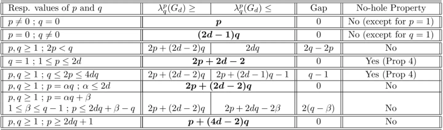
Resp. values of p and q λp
q(Gd) ≥ λpq(Gd) ≤ Gap No-hole Property
p6= 0 ; q = 0 p 0 No (except for p = 1) p= 0 ; q 6= 0 (2d − 1)q 0 No (except for q = 1) p, q≥ 1 ; 2p < q 2p + (2d − 2)q 2dq 2q − 2p No q= 1 ; 1 ≤ p ≤ 2d 2p + 2d − 2 0 Yes (Prop 4) p, q≥ 1 ; q ≤ 2p ≤ 4dq 2p + (2d − 2)q 2p + (2d − 1)q − 1 q− 1 Yes (Prop 4) p, q≥ 1 ; p = αq ; α ≤ 2d 2p + (2d − 2)q 0 No p, q≥ 1 ; p = αq + β 1 ≤ β ≤ q − 1 ; p ≤ 2dq + β − q 2p + (2d − 2)q 2p + 2dq − 2β 2(q − β) No p, q≥ 1 ; p ≥ 2dq + 1 p+ (4d − 2)q 0 No
Table 1: L(p, q) labeling of Gd : Summary of the results
Moreover, in the case 1 ≤ q ≤ 2p ≤ 4dq, for sufficiently large grids (that is, when the xis
are large enough for each 1 ≤ i ≤ d), the coloring we propose to achieve an L(p, q) labeling satis-fies the no-hole property, that is all the colors in the range [0; 2p + 2(d − 1)q − 1] are used. This is the purpose of the following Proposition 4 below.
Proposition 4 (No-hole property of L(p, q) labeling of Gd, when 1 ≤ q ≤ 2p ≤ 4dq) Let
d≥ 1. In that case, when 1 ≤ q ≤ 2p ≤ 4dq, there exists a no-hole L(p, q) labeling of Gd such that
λpq(Gd) = 2p + (2d − 1)q − 1.
Proof : In Proof of Lemma 2, in the case 1 ≤ q ≤ 2p ≤ 4dq, we assign to any vertex u = (x1, x2. . . xd) color c(u) = (P
d
i=1(p + (i − 1)q)xi) mod (2p + (2d − 1)q). Let U = {uk =
(0, 0 . . . 0, 2k)|1 ≤ k ≤ 2p+(2d−1)q} : in other words, in any vertex uk, 1 ≤ k ≤ 2p+(2d−1)q, only
the d-th coordinate xdis different from 0, and xd = 2k. In that case, c(uk) ≡ (p+(d−1)q)·2k mod
2p+(2d−1)q by definition. However, (p+(d−1)q)·2k = (k−1)·(2p+(2d−1)q)+(2p+2(d−1)q−k), hence c(uk) ≡ 2p + 2(d − 1)q − k, since k ≤ 2p + (2d − 1)q. Since the grid Gd is supposed to be
sufficiently large, there is no restriction on the choice of xd, and thus on the choice of k. Hence,
one can see that each vertex uk of U is assigned a unique color c(uk) = 2p + (2d − 1)q − k. Since k
takes all the values between 1 and 2p + (2d − 1)q, we conclude that the vertices of U are assigned colors that take all the values in the range [0; 2p + (2d − 1)q − 1]. Hence, the proposed labeling is a no-hole L(p, q) labeling of Gd. 2
Clearly, in the other cases, the proposed L(p, q) labelings cannot be no-hole labelings, be-cause some colors are forbidden. Indeed, in the case 2 ≤ 2p < q, colors are taken in the set {0, q, 2q, . . . 2dq}, thus it cannot be a no-hole coloring. In the case p ≥ 2dq + 1, the colors ranging in the interval [(2d − 1)q + 1; p + (2d − 1)q − 1] are forbidden, thus the coloring we suggest cannot be no-hole.
Table 1 summarizes the results obtained in Section 2 concerning bounds for the L(p, q) coloring of Gd, for all the possible cases. In this table, we give the lower and upper bounds for λpq(Gd) ;
they are given in bold characters when the bounds coincide. We also mention the gap between the upper and lower bounds when they do not coincide. Finally, in the rightmost column, we state whether the no-hole property holds for the colorings suggested in this paper.
We also mention that the upper bounds we obtain here concerning the L(p, q) labeling of Gd
are also upper bounds for the L(p, q) labeling of hypercubes of dimension d, Hd. Indeed, Hd is
isomorphic to the grid Gd where each xi can take only two values (Hence, there are only two
vertices lying in each dimension of the grid). L(2, 1) labeling of the hypercube of dimension d has been studied in [GY92], where the authors proved that d + 3 ≤ λ2
was conjectured that λ2
1(Hd) = d + 3. The upper bound has been improved later in cite [WGM95]
thanks to a technique coming from coding theory. However, to our knowledge, the L(p, q) labeling of Hd has not been studied for general p and q. Hence, the results stated in Corollary 1 below
constitute a first approach for tackling this problem. However, these upper bounds need to be improved.
Corollary 1 (L(p, q) labeling of d-dimensional Hypercubes, for any value of p, q, d ≥ 1) Let p ≥ 1 and d ≥ 1. Then :
• λp0(Hd) = p when p, d ≥ 1 • λ0 q(Hd) ≤ (2d − 1)q when q, d ≥ 1 • λp q(Hd) ≤ 2dq when 2 ≤ 2p < q • λp q(Hd) ≤ 2p + (2d − 1)q − 1 when 1 ≤ q ≤ 2p ≤ 4dq • λp
q(Hd) ≤ 2p + (2d − 2)q when p = αq with p, q ≥ 1 and α ≤ 2d
• λp
q(Hd) ≤ 2p + 2dq − 2β when p, q ≥ 1, p = αq + β with 1 ≤ β ≤ q − 1 and p ≤ 2dq + β − q
• λp
q(Hd) ≤ p + (4d − 2)q when p ≥ 2dq + 1
We note that we get the equality λp0(Hd) = p in the case q = 0 since we need to have a gap of
at least p between any vertex colored 0 and its neighbor.
We finish this section by mentioning a result for the labeling of Gd with k constraints, each
equal to 1. This labeling is usually denoted as an L(~1k) labeling. The results we give here are
derived from a study initiated in [FGR03]. This is the purpose of the remark below.
Remark 1 (L(~1k) labeling of Gd) In [FGR03], the authors have considered the k-distance
col-oring in the d-dimensional grid Gd. k-distance coloring of a graph G is a coloring of its vertices
such that two vertices lying at distance less than or equal to k must be assigned different colors. Clearly, k-distance coloring is equivalent to the L(~1k) labeling, that is the L(1, 1 . . . 1) labeling with
k constraints on the distances, each equal to 1).
In their paper, the authors prove that λ11(Gd) = 2d for any d ≥ 1. This result appears as a
particular result of Theorem 1, when p = q = 1.
Another result from [FGR03] addresses the L(~1k) labeling problem in the 2-dimensional grid
G2, for any k ≥ 1. Their result is the following :
• if k is even, then λ(~1k)[G2] =(k+1) 2 +1 2 − 1 ; • if k is odd, then λ(~1k)[G2] =(k+1) 2 2 − 1.
We note that this result has also been independently given in [BPT02].
3
Conclusion
In this paper, we have addressed the frequency assignment problem with constraints on the dis-tances. We have first given general bounds for the λ number when k constraints are given for the kfirst distances.
We have also addressed the problem of the L(p, q) labeling in d-dimensional grids. These re-sults are optimal in the cases p = 0, q = 0, p ≥ 2dq + 1, p = αq with 1 ≤ α ≤ 2d, and also in the case q = 1 (where in the latter case, our result answers an open question from [DMP+02], and
generalizes results from [DMP+02] and [BPT00]). The only case where the result is not optimal
case, the lower and upper bounds for λp
q(Gd) differ by min{q − 1, 2(q − β)} (in the case 2p ≥ q), or
by 2q − 2p ≤ 2q − 2 (in the case 2p < q). We proved that the coloring of the vertices we propose in the case 1 ≤ q ≤ 2p ≤ 4dq, though not necessarily optimal (when q ≥ 2), is a no-hole coloring. We have also derived some upper bounds for the L(p, q) coloring of d-dimensional hypercubes.
Finally, we wish to end this paper by suggesting that, using similar techniques, the results presented here could be extended to the L(p, q, r) labeling problem in d-dimensional grids Gd.
References
[BKTvL00] H.L. Bodlaender, T. Kloks, R.B. Tan, and J. van Leeuwen. λ-coloring of graphs. In Proc. STACS 2000 : 17th Annual Symposium on Theoretical Aspect of Computer Science, volume 1770, pages 395–406. Lecture Notes Computer Science, Springer-Verlag Berlin, 2000.
[BPT00] A.A Bertossi, C.M. Pinotti, and R.B. Tan. Efficient use of radio spectrum in wireless networks with channel separation between close stations. In Proc. DIAL M for Mo-bility 2000 (Fourth International Workshop on Discrete Algorithms and Methods for Mobile Computing and Communications), 2000.
[BPT02] A.A Bertossi, C.M. Pinotti, and R.B. Tan. Channel assignment with separation for special classes of wireless networks : Grids and rings. In Proc. IPDPS’02 (Interna-tional Parallel and Distributed Processing Symposium), pages 28–33. IEEE Computer Society, 2002.
[CK96] G.J. Chang and D. Kuo. The L(2, 1)-labeling on graphs. SIAM J. Discrete Math., 9:309–316, 1996.
[CKK+02] G.J. Chang, W.-T. Ke, D. Kuo, D.D.-F. Liu, and R.K. Yeh. On L(d, 1)-labelings of
graphs. Discrete Mathematics, 220:57–66, 2002.
[CP01] T. Calamoneri and R. Petreschi. L(2, 1)-labeling of planar graphs. In Proc. DIAL M for Mobility 2001 (Fifth International Workshop on Discrete Algorithms and Methods for Mobile Computing and Communications), pages 28–33, 2001.
[DMP+02] A. Dubhashi, S. MVS, A. Pati, S. R., and A.M. Shende. Channel assignment for
wireless networks modelled as d-dimensional square grids. In Proc. IWDC’02 (Inter-national Workshop on Distributed Computing), volume 2571, pages 130–141. Lecture Notes in Computer Science - Springer Verlag, 2002.
[FGR03] G. Fertin, E. Godard, and A. Raspaud. Acyclic and k-distance coloring of the grid. Information Processing Letters, 87(1):51–58, 2003.
[FKK01] J. Fiala, T. Kloks, and J. Kratochvil. Fixed-parameter complexity of λ-labelings. Discrete Applied Mathematics, 113:59–72, 2001.
[FKP01] J. Fiala, J. Kratochvil, and A. Proskurowski. Distance constrained labelings of precol-ored trees. In Proc. 7th Italian Conference, ICTCS 2001, volume 2202, pages 285–292. Lecture Notes in Computer Science - Springer Verlag, 2001.
[GY92] J.R. Griggs and R.K. Yeh. Labeling graphs with a condition at distance two. SIAM J. Discrete Math., 5:586–595, 1992.
[Hal80] W.K. Hale. Frequency assignment : theory and applications. Proc. IEEE, 60:1497– 1514, 1980.
[Jha00] P.K. Jha. Optimal L(2, 1)-labeling of cartesian products of cycles with an application to independent domination. IEEE Trans. Circuits & Systems I: Fundamental Theory and Appl., 47:1531–1534, 2000.
[JNS+00] P.K. Jha, A. Narayanan, P. Sood, K. Sundaram, and V. Sunder. On L(2, 1)-labeling
of the cartesian product of a cycle and a path. Ars Combin., 55:81–89, 2000. [Kra] D. Kral. Coloring powers of chordal graphs. SIAM J. Discr. Math. To appear. [MS02] M. Molloy and M.R. Salavatipour. Frequency channel assignment on planar networks.
In In Proc. 10th Annual European Symposium (ESA 2002), Rome, Italy, September 2002, volume 2461, pages 736–747. Lecture Notes Computer Science, Springer-Verlag Berlin, 2002.
[Sak94] D. Sakai. Labeling chordal graphs with a condition at distance two. SIAM J. Discrete Math., 7:133–140, 1994.
[WGM95] M. Whittlesey, J. Georges, and D.W. Mauro. On the λ-number of Qn and related