A review of vertical ground heat exchanger sizing tools including an inter-model comparison

Titre:

Title

:

A review of vertical ground heat exchanger sizing tools including an

inter-model comparison

Auteurs:

Authors

: Michel Bernier

Date: 2019

Type:

Référence:

Citation

:

Bernier, M. (2019). A review of vertical ground heat exchanger sizing tools including an inter-model comparison. Renewable and Sustainable Energy

Reviews, 110, p. 247-265. doi:10.1016/j.rser.2019.04.045

Document en libre accès dans PolyPublie

Open Access document in PolyPublie

URL de PolyPublie:

PolyPublie URL: https://publications.polymtl.ca/3961/

Version: Version finale avant publication / Accepted version_{Révisé par les pairs / Refereed} Conditions d’utilisation:

Terms of Use: CC BY-NC-ND

Document publié chez l’éditeur officiel

Document issued by the official publisher

Titre de la revue:

Journal Title: Renewable and Sustainable Energy Reviews (vol. 110) Maison d’édition:

Publisher: Elsevier URL officiel:

Official URL: https://doi.org/10.1016/j.rser.2019.04.045 Mention légale:

Legal notice:

Ce fichier a été téléchargé à partir de PolyPublie, le dépôt institutionnel de Polytechnique Montréal

This file has been downloaded from PolyPublie, the institutional repository of Polytechnique Montréal

1

A review of vertical ground heat

exchanger sizing tools including an

inter-model comparison

by

Mohammadamin Ahmadfard

and

Michel Bernier

_{, PE, Ph.D.}

Polytechnique Montréal

Department of Mechanical Engineering

2500 chemin de Polytechnique

Montréal, Canada, H3T 1J4

Accepted manuscript

Declarations of interest: None

₁

2

A review of vertical ground heat exchanger sizing tools including an

inter-model comparison

Abstract

This paper attemps to fill a gap in the literature on ground heat exchanger sizing tools which are routinely used but have not been recently compared against each other. First, a comprehensive review of the governing equations of these tools is presented. The tools are then classified into five levels (𝐿𝐿0 to 𝐿𝐿4) according to their level of complexity from tools based on rules-of-thumb (𝐿𝐿0) to those using annual hourly simulations (𝐿𝐿4). Then this study presents a methodology for comparing vertical ground heat exchanger sizing tools. After a review of available tests, four test cases are proposed to cover the full spectrum of conditions from single boreholes to large bore fields with various annual ground thermal imbalances. This is followed by an inter-model comparison of twelve sizing tools including some commercially-available software programs and various forms of the ASHRAE sizing equation. In one of the tests on a single borehole subjected to a one-hour peak load duration, it is shown that the minimum and maximum lengths obtained by the various tools are 39.1 m and 59.7 m. Tools that include short-term effects tend to calculate smaller lengths while longer lengths are predicted by tools that evaluate effective ground thermal resistances using the cylindrical heat source solution. In another test involving a large annual ground imbalance on a 5×5 borehole field, it is shown that results vary from 93.0 m to 128.9 m among the twelve tools. A group of seven tools, including 𝐿𝐿2, 𝐿𝐿3, and 𝐿𝐿4 tools are in good agreement with a minimum of 121.0 m and a maximum of 128.9 m. Two tools have determined lengths that are much lower than the rest of the tools (103.9 and 93.0 m). Clearly, these two tools cannot properly account for borehole thermal interaction caused by large annual imbalanced loads.

3

1. Introduction

Ground heat exchanger sizing tools use different calculation procedures to obtain the required bore field length for a given set of ground loads. The last serious attempt to compare these design tools is about two decades old. Since then, tools have been improved and new ones have been introduced. The goal of this paper is to provide an updated inter-model comparison of twelve tools. Aside from this end result, this study classifies the various calculation procedures into five levels based on their complexity. It also provides a rigorous methodology to compare the various tools and proposes test cases for a range of conditions.

A ground source heat pump (GSHP) system equipped with vertical ground heat exchangers (GHE) is depicted in Figure 1. This system is composed of a series of boreholes and heat pumps which provide heating and cooling to a building. The bore field consists of a number of boreholes, 𝑁𝑁𝑏𝑏, with length 𝐻𝐻, spaced apart by a distance 𝐵𝐵 and buried at a depth

𝐷𝐷. The overall length of the bore field, 𝐿𝐿, is thus equal to 𝑁𝑁𝑏𝑏× 𝐻𝐻. Boreholes have a radius 𝑟𝑟𝑏𝑏 and typically contain one

or two U-tubes with a thermal conductivity, 𝑘𝑘𝑝𝑝. In the case of Figure 1, two pipes (one U-tube) with internal and external

diameters, 𝑟𝑟𝑝𝑝,𝑖𝑖 and 𝑟𝑟𝑝𝑝,𝑜𝑜 , are used. They are separated by a distance 2𝑑𝑑𝑝𝑝. The borehole is usually filled with grout with a

thermal conductivity, 𝑘𝑘𝑔𝑔𝑟𝑟 , and a thermal capacity, 𝑀𝑀𝑀𝑀𝑝𝑝𝑔𝑔𝑔𝑔. The ground is characterized by its thermal conductivity, 𝑘𝑘𝑔𝑔,

thermal diffusivity, 𝛼𝛼𝑔𝑔, and undisturbed temperature, 𝑇𝑇𝑔𝑔.

Figure 1: Schematic representation of a ground-source heat pump system (left) and a borehole cross-section with one

U-tube (right)

Boreholes are typically connected in parallel. The fluid inlet temperatures and flow rates are usually assumed to be identical for all boreholes. Assuming negligible heat gains/losses in the piping between the boreholes and the heat

Building Load Heat pumps Pump Tin,hp Tout,hp Grout-kgr, MCpgr Pipe-kp D H B 2rb 2dp 2rp,o 2rp,i Ground kg, Tg, αg

4

pumps, the bore field outlet temperature is equal to the heat pump inlet temperature, 𝑇𝑇𝑖𝑖𝑛𝑛,ℎ𝑝𝑝, and the heat pump outlet

temperature, 𝑇𝑇𝑜𝑜𝑜𝑜𝑜𝑜,ℎ𝑝𝑝, is equal to the bore field inlet temperature. The flow rate in each borehole is equal to 𝑚𝑚̇𝑓𝑓/𝑁𝑁𝑏𝑏, where

𝑚𝑚̇𝑓𝑓 is the total bore field flow rate. For commercially available heat pumps, 𝑇𝑇𝑖𝑖𝑛𝑛,ℎ𝑝𝑝 can be as low as −7℃ in heating and

as high as 45℃ in cooling. However, designers most often plan their system so that 𝑇𝑇𝑖𝑖𝑛𝑛,ℎ𝑝𝑝 ≥ 0℃ in heating and 𝑇𝑇𝑖𝑖𝑛𝑛,ℎ𝑝𝑝≤

35℃ in cooling. These two limiting temperatures will be referred to 𝑇𝑇𝐿𝐿 and 𝑇𝑇𝐻𝐻, respectively. Unlike HVAC equipment

which are typically sized only for peak load conditions, bore field sizing has to account for the thermal history of heat injection/collection into the ground and the period of the year when the system starts to operate [1].

A number of input parameters, listed in Table 1, need to be determined prior to using sizing tools. Building or ground loads are generally determined using separate tools. Inaccurate loads will have an impact on the accuracy of 𝐿𝐿. For instance, Bernier [2] has shown, for a particular case, that an uncertainty of ± 10% on the peak, monthly and annual ground loads (𝑞𝑞_ℎ, 𝑞𝑞_𝑚𝑚, 𝑞𝑞_𝑦𝑦 in equation 4 – to be described later) translates into a cumulative uncertainty of ± 8.9% on 𝐿𝐿. The duration of peak loads has also an influence on 𝐿𝐿: typical values range from 4 to 6 hours. The next required input parameters are the target heat pump inlet temperature limits, 𝑇𝑇𝐻𝐻 and 𝑇𝑇𝐿𝐿, that should not be exceeded during the expected

lifetime of the system. The user has also to decide on the bore field geometry which is often dictated by the available land area. Cimmino and Bernier [3] have shown that borehole placement within a given rectangular land area is not crucial in terms of total borehole length. An accurate value of the ground thermal conductivity is important to properly size a bore field while the ground thermal diffusivity is less important. Bernier [2] has shown that a ± 10% uncertainty on 𝑘𝑘𝑔𝑔 and 𝛼𝛼𝑔𝑔 lead, respectively, to uncertainties of ± 7.1%, and ± 1.0% on the bore field length for a particular case. An

accurate value for the ground temperature is also important and when it’s value is close to 𝑇𝑇𝐻𝐻 or 𝑇𝑇𝐿𝐿, longer boreholes

are required. The borehole characteristics need to be carefully selected to optimize the borehole thermal resistance and the overall length. Some sizing tools account for borehole thermal capacity and in these cases, the thermal capacities of the pipes, the fluid and the grout are required. If building loads are used as inputs in sizing tools, heat pump coefficient of performances (𝑀𝑀𝐶𝐶𝐶𝐶𝐶𝐶) in heating and cooling are required to calculate ground loads. The simpler methods will only require 𝑀𝑀𝐶𝐶𝐶𝐶𝐻𝐻 and 𝑀𝑀𝐶𝐶𝐶𝐶𝐶𝐶 at 𝑇𝑇𝐿𝐿 and 𝑇𝑇𝐻𝐻 while more elaborate tools will evaluate 𝑀𝑀𝐶𝐶𝐶𝐶𝐻𝐻 and 𝑀𝑀𝐶𝐶𝐶𝐶𝐶𝐶 as a function of 𝑇𝑇𝑖𝑖𝑛𝑛,ℎ𝑝𝑝.

The selection of a flow rate has an influence on borehole heat transfer and on the ∆𝑇𝑇 across the borehole. A high flow rate reduces the borehole thermal resistance and the ∆𝑇𝑇 but increases pumping power. Low flow rates may lead to

5

laminar flows in the borehole pipes which should be avoided at peak ground load conditions. For sizing purposes, the flow rate is typically around 0.05-1.0 L/s per kW of peak load. The required borehole length is not necessarily obtained at the end of the design period (typically 10 to 20 years). Indeed, Monzó et al. [1] have shown that the maximum length might be required during the first year of operation depending on the starting month of operation.

Table 1: Required input parameters for most sizing tools

Building or ground loads and peak load duration Target temperature limits for heat pumps (𝑇𝑇𝐿𝐿 and 𝑇𝑇𝐻𝐻)

Bore field geometry (number of boreholes and location) Ground thermal properties (𝑘𝑘𝑔𝑔 𝛼𝛼𝑔𝑔 and 𝑇𝑇𝑔𝑔)

Borehole characteristics (geometry, thermal properties) Heat pump characteristics (𝑀𝑀𝐶𝐶𝐶𝐶𝐻𝐻 and 𝑀𝑀𝐶𝐶𝐶𝐶𝐶𝐶)

Flow rate Design period

Starting month of operation

Sizing tools take different paths to obtain 𝐿𝐿 with various levels of complexity and accuracy. Spitler and Bernier [4] have identified five such levels (𝐿𝐿0 to 𝐿𝐿4). Figure 2 presents typical calculation sequences associated with tools in the 𝐿𝐿1 to 𝐿𝐿4 categories. These levels are described in the next section including a presentation of some available sizing tools within each level. This is followed by a literature review on comparisons of bore field sizing tools. Then, a series of test cases are proposed. Finally, these test cases are used in an inter-model comparison of several existing tools.

6

Figure 2: Typical steps required to size a bore field for a) 𝐿𝐿1 and 𝐿𝐿2 methods, b) 𝐿𝐿3 and 𝐿𝐿4 methods with building

loads as input, and c) 𝐿𝐿3 and 𝐿𝐿4 methods with ground loads as inputs.

Heat pump Building loads and peak

duration Guess value for L Borehole thermal resistance Ground loads Update L 1 2 Ground thermal response factors Evaluation of Tin,hp 3 4 5 6 7 Tf reached TL or TH

during life-span and not exceed them?

End Start

Y

N

Ground loads and peak duration Update L 1 2 Ground thermal response factors Evaluation of Tin,hp 3 4 5 Start Building loads and peak

duration Heat pump COPH at TL and COPC at TH

Ground loads Guess value for L Borehole thermal resistance Update L 1 2 Ground thermal response factors and T_p

New value of L 3 4 5 6 7 Start b. COP Converged? N Y

Guess value for L Borehole thermal

resistance

Tf reached TLor TH

during life-span and not exceed them?

End Y N c. Converged End Y N a. 8 8 6

7

2. Categories of sizing tools

Level 𝐿𝐿0 tools are simple rules-of-thumb. They typically relate the borehole length to the building peak heating or cooling loads or installed capacity, typically expressed as W/m or ft/ton. Spitler and Bernier [4] mention that 𝐿𝐿0 tools are mostly used for small systems in heating only applications. They are bound to give erroneous results in large systems where borehole-to-borehole thermal interaction, caused by ground thermal imbalance and/or small borehole spacing, is large. Also, they do not consider the borehole thermal resistance. They should only be used as a reality check for more advanced sizing tools.

Excluding 𝐿𝐿0 tools, most sizing methods are derived from Equation 1: 𝐿𝐿 = ∑ 𝑞𝑞_𝑇𝑇𝑁𝑁𝑖𝑖=1 𝑖𝑖𝑅𝑅𝑖𝑖+ 𝑞𝑞ℎ𝑅𝑅𝑏𝑏

𝑚𝑚− (𝑇𝑇𝑔𝑔+ 𝑇𝑇𝑝𝑝) (1)

where 𝑞𝑞_𝑖𝑖 is a ground thermal pulse associated with a certain time period, 𝑅𝑅𝑖𝑖 is the corresponding ground thermal response

which takes the form of an effective ground thermal resistance, 𝑞𝑞_ℎ is the peak ground thermal pulse, 𝑅𝑅𝑏𝑏 is the borehole

thermal resistance, 𝑇𝑇𝑚𝑚 is the mean borehole fluid temperature (=(𝑇𝑇𝑖𝑖𝑛𝑛𝐻𝐻𝐶𝐶+ 𝑇𝑇𝑜𝑜𝑜𝑜𝑜𝑜𝐻𝐻𝐶𝐶)/2)), and 𝑇𝑇𝑝𝑝 is a temperature penalty

to account for borehole-to-borehole thermal interaction. In some methods, this thermal interaction is included in 𝑅𝑅𝑖𝑖 values and for such methods, 𝑇𝑇𝑝𝑝 = 0. Equation 1 can be used for heating or cooling applications with appropriate

signs for ground loads (negative when heat is extracted from the ground). 2.2. L1 – Two pulses –peak heating and cooling loads

𝐿𝐿1 methods use two heat pulses which are either the maximum heating and cooling heat pump capacities or the building peak heating and cooling loads. They are somewhat outdated but it is interesting to present them from an historical perspective. 𝐿𝐿1 methods have been described by Bose et al. [5], OSU [6], and Kavanaugh [7]. With reference to Figure 2a, a 𝐿𝐿1 tool would typically go through the six step process starting with the peak building loads or in some cases with the installed heat pump capacity. In step 2, values of 𝑀𝑀𝐶𝐶𝐶𝐶𝐻𝐻 and 𝑀𝑀𝐶𝐶𝐶𝐶𝐶𝐶 are determined based on values of 𝑇𝑇𝐿𝐿 and 𝑇𝑇𝐻𝐻 and

used in the determination of the ground loads in step 3. Heat pump compressor power is either added or subtracted from the building to obtain ground loads. Thus, the heat pump 𝑀𝑀𝐶𝐶𝐶𝐶, which is the ratio of the capacity (heating or cooling) over compressor power, has an impact on bore field sizing. For example, the overall length of a bore field will decrease with an increase of heat pump 𝑀𝑀𝐶𝐶𝐶𝐶 when a bore field is sized in cooling. Conversely, when a bore field is sized for

8

heating conditions, an increase in the 𝑀𝑀𝐶𝐶𝐶𝐶 value will lead to an increase in the bore field length. Rudimentary values, by today’s standards, of the borehole thermal resistance and ground thermal response factors are typically evaluated in steps 4 and 6. Finally, 𝐿𝐿 is obtained directly in step 7 and iterations on 𝐿𝐿 are generaly not required. 𝐿𝐿1 tools are perhaps best explained by examining the so-called IGSHPA method which is thoroughly described by Bose et al. [5]. This method follows the sequence presented in Figure 2a except that building loads are replaced by heat pump capacities in step 1. In this method, the lengths in heating (𝐿𝐿𝐻𝐻) and cooling (𝐿𝐿𝑀𝑀) are determined using Equation 2 with the longest of

the two giving the total required borehole length, 𝐿𝐿. As shown in Equation 2, the heat pump capacities in heating and cooling, 𝑀𝑀𝐶𝐶𝑝𝑝𝐻𝐻 and 𝑀𝑀𝐶𝐶𝑝𝑝𝐶𝐶, are multiplied by a factor involving 𝑀𝑀𝐶𝐶𝐶𝐶𝐶𝐶 in heating and cooling (𝑀𝑀𝐶𝐶𝐶𝐶𝐻𝐻 and 𝑀𝑀𝐶𝐶𝐶𝐶𝐶𝐶) to obtain

peak ground loads in heating and cooling, respectively. These loads are then multiplied by the sum of the pipe (borehole) resistance, 𝑅𝑅𝑝𝑝, and of the ground thermal response (ground thermal resistance), 𝑅𝑅𝐶𝐶. This last value is multiplied by the

runtime fraction, (𝑅𝑅𝑜𝑜𝑛𝑛𝑓𝑓,𝐻𝐻 or 𝑅𝑅𝑜𝑜𝑛𝑛𝑓𝑓,𝑀𝑀). The denominator of Equation 2.c is the difference between 𝑇𝑇𝑔𝑔 and 𝑇𝑇𝐿𝐿 in heating

or between 𝑇𝑇𝐻𝐻 and 𝑇𝑇𝑔𝑔 in cooling.

𝐿𝐿𝐻𝐻= 𝑀𝑀𝐶𝐶𝑝𝑝_𝐻𝐻(𝑀𝑀𝐶𝐶𝐶𝐶𝐻𝐻− 1) 𝑀𝑀𝐶𝐶𝐶𝐶𝐻𝐻 �𝑅𝑅𝑝𝑝+ 𝑅𝑅𝐶𝐶𝑅𝑅𝑜𝑜𝑛𝑛𝑓𝑓,𝐻𝐻� �𝑇𝑇𝑔𝑔− 𝑇𝑇𝐿𝐿� (2.a) 𝐿𝐿𝑀𝑀= 𝑀𝑀𝐶𝐶𝑝𝑝_𝑀𝑀(𝑀𝑀𝐶𝐶𝐶𝐶𝑀𝑀+ 1) 𝑀𝑀𝐶𝐶𝐶𝐶𝑀𝑀 �𝑅𝑅𝑝𝑝+ 𝑅𝑅𝐶𝐶𝑅𝑅𝑜𝑜𝑛𝑛𝑓𝑓,𝑀𝑀� 𝑀𝑀𝐶𝐶𝐶𝐶𝑀𝑀�𝑇𝑇𝐻𝐻− 𝑇𝑇𝑔𝑔� (2.b) 𝐿𝐿 = max(𝐿𝐿𝐻𝐻, 𝐿𝐿𝐶𝐶) (2.c)

The ground thermal resistance, 𝑅𝑅𝐶𝐶, is determined using the infinite line source solution. Its value depends on the time

period over which the ground load is applied. Also, spatial superposition can be used to account for borehole thermal interaction as discussed by Bose et al. [5]. The pipe resistance, 𝑅𝑅𝑝𝑝, is the ancestor of the modern borehole thermal

resistance. For a U-tube geometry, it is approximated using an equivalent diameter.

Equation 2 is applied for winter and summer design periods. 𝑀𝑀𝐶𝐶𝑝𝑝𝐻𝐻 and 𝑀𝑀𝐶𝐶𝐶𝐶𝐻𝐻 are evaluated at 𝑇𝑇𝐿𝐿 while 𝑀𝑀𝐶𝐶𝑝𝑝𝐶𝐶 and 𝑀𝑀𝐶𝐶𝐶𝐶𝐶𝐶

are evaluated at 𝑇𝑇𝐻𝐻. Accurate values of 𝐿𝐿 are largely dependent on the selection of the design period duration, which

influences 𝑅𝑅𝐶𝐶, and on the estimation of the run time fraction for the heat pumps during that period, (𝑅𝑅𝑜𝑜𝑛𝑛𝑓𝑓,𝐻𝐻 or 𝑅𝑅𝑜𝑜𝑛𝑛𝑓𝑓,𝑀𝑀).

9

The ground thermal resistances evaluated by this approach are not precise for long-term estimations since the one-dimensional (radial) infinite line source solution does not account for increased heat transfer at the borehole extremities which can be important after several months of operation. These simplifications, as explained by Cane and Forgas [8] and Caneta [9] lead to borehole oversizing.

2.3. L2 – Three pulse methods

𝐿𝐿2 methods use temporal superposition of three successive load pulses to size bore fields. These pulses are: i) peak ground load; ii) average monthly ground load during the month in which the peak load occurs; and iii) the yearly average ground load. With reference to Equation 1, the summation term would then involve three terms. Each of these pulses is applied over a certain time period which typically corresponds to: 4 to 6 hours for the peak load; 30 days for the monthly load; and 10 years for the yearly load. Thus, the lengths 𝐿𝐿 determined with 𝐿𝐿2 methods are the lengths required to reach the temperature limits (𝑇𝑇𝐿𝐿 or 𝑇𝑇𝐻𝐻) when the bore field is subjected to 10 years of the yearly average ground load followed

by 30 days of the average monthly ground load and finally 4 o 6 hours of the peak ground load.

With reference to Figure 2a, 𝐿𝐿2 methods start either at step 1 or 3. Step 1 involves the determination of three building loads associated with the three thermal pulses, i.e. the peak building loads in heating and cooling and their duration, the monthly averaged building loads in heating and cooling during the peak month and the total annual heating/cooling loads. Then, peak ground loads are obtained in step 3 using the 𝑀𝑀𝐶𝐶𝐶𝐶𝐻𝐻 and 𝑀𝑀𝐶𝐶𝐶𝐶𝐶𝐶 values determined in step 2. Monthly

ground loads are evaluated as a fraction (often called the Part-Load Factor – 𝐶𝐶𝐿𝐿𝑃𝑃) of the peak loads and the annual average ground load can be calculated using the concept of equivalent full load hours using the peak loads and 𝑀𝑀𝐶𝐶𝐶𝐶𝐻𝐻

and 𝑀𝑀𝐶𝐶𝐶𝐶𝐶𝐶 determined in step 2. Then, three ground thermal response factors (or ground thermal resistances) and 𝑇𝑇𝑝𝑝 are

evaluated in step 6. As shown below in the description of some 𝐿𝐿2 tools, these values are determined using either the infinite cylindrical heat source analytical solution or g-functions. If the ground thermal resistances (and 𝑇𝑇𝑝𝑝) depend on

the borehole length then an iterative process is required and ground thermal response factors are re-evaluated until convergence as indicated in Figure 2a. In some methods, the borehole thermal resistance depends also on 𝐿𝐿, in which case the calculations are reinitiated in step 4 as indicated by the dotted line in Figure 2a. Three 𝐿𝐿2 methods (and their variations) will now be reviewed.

10

ASHRAE sizing equation

Equation 3 will be referred here as the ASHRAE sizing equation. This equation first appeared in the 1995 ASHRAE Handbook-Applications [10] and in a paper by Kavanaugh [11] and is still used in the latest version [12] of the ASHRAE Handbook-Applications. Earlier versions of these equations were presented by Kavanaugh [7, 13]. Equation 3 can either be used for heating or cooling applications: 𝑇𝑇𝑖𝑖𝑛𝑛,ℎ𝑝𝑝 is replaced by 𝑇𝑇𝐿𝐿 or 𝑇𝑇𝐻𝐻, the design temperature limits in heating and

cooling, respectively, and 𝑇𝑇𝑜𝑜𝑜𝑜𝑜𝑜,ℎ𝑝𝑝 is determined from an energy balance on the bore field.

𝐿𝐿 =𝑞𝑞𝑦𝑦𝑅𝑅𝑦𝑦+ (𝑞𝑞ℎ− 𝑊𝑊)(𝑅𝑅𝑏𝑏+ 𝐶𝐶𝐿𝐿𝑃𝑃𝑚𝑚𝑅𝑅𝑚𝑚+ 𝑅𝑅ℎ𝑃𝑃𝑠𝑠𝑠𝑠) 𝑇𝑇𝑔𝑔−�𝑇𝑇𝑖𝑖𝑖𝑖,ℎ𝑝𝑝+ 𝑇𝑇₂ 𝑜𝑜𝑜𝑜𝑜𝑜,ℎ𝑝𝑝�− 𝑇𝑇𝑝𝑝

(3) In Equation 3, the annual, monthly and peak load pulses are given by: i) 𝑞𝑞_𝑦𝑦, the net annual average heat transfer to the ground, ii) �𝑞𝑞_ℎ− 𝑊𝑊�𝐶𝐶𝐿𝐿𝑃𝑃𝑚𝑚 , the monthly average heat transfer to the ground, and iii) �𝑞𝑞ℎ− 𝑊𝑊�, the peak heat transfer

rate to the ground. Note that 𝑞𝑞_𝑦𝑦 is a ground load and that 𝑞𝑞_ℎ is a building load which is converted into a ground load by subtracting the compressor power at peak load, 𝑊𝑊. 𝐶𝐶𝐿𝐿𝑃𝑃𝑚𝑚 is the part load factor during the design month and finally 𝑃𝑃𝐶𝐶𝑠𝑠

is the short circuit heat loss factor in the borehole. This last value, which is typically very close to 1, is tabulated in the ASHRAE handbook [12]. 𝑅𝑅𝑦𝑦, 𝑅𝑅𝑚𝑚 and 𝑅𝑅ℎ are the yearly, monthly and hourly effective ground thermal resistances which

are evaluated using the infinite cylindrical source (ICS) analytical solution. With the use of the ICS, the ASHRAE equation is relatively simple to calculate as the ground thermal resistances do not depend on the heat exchanger length and so the result can be determined directly without iterations. However, the use of the ICS implies that borehole-to-borehole thermal interaction is not accounted for. The equation thus needs a correction factor, referred to as a temperature penalty, 𝑇𝑇𝑝𝑝.

Values of 𝑇𝑇𝑝𝑝 are tabulated in the ASHRAE Handbook [12] for a limited number of bore field configurations and annual

ground thermal imbalances (𝑞𝑞_𝑦𝑦). These values are based on a calculation procedure developed by Kavanaugh and Rafferty [14] which was recently slightly modified [15] to account for heat transfer from the bottom of the bore field. This last method of calculating 𝑇𝑇𝑝𝑝will be used later in the inter-model comparison. With this method, 𝑇𝑇𝑝𝑝 can be regarded

11

thermal imbalance. This method of calculating 𝑇𝑇𝑝𝑝 has been criticized by a number of authors (e.g. Bernier et al. [16],

Fossa [17]) and has been shown to underestimate 𝑇𝑇𝑝𝑝.

As for the determination of the borehole thermal resistance, 𝑅𝑅𝑏𝑏, the ASHRAE handbook proposes a table of 𝑅𝑅𝑏𝑏 values

for two (one U-tube) and four pipes (two U-tubes) for three grout conductivities, three fluid flow regimes (laminar, transition, and fully turbulent), three U-tubes sizes, and three bore diameters. Various pipe locations within the borehole are also considered. Reported values are calculated using a publicly-available spreadsheet program [18]. The ASHRAE equation has been implemented in a tool called GCHPcalc [11].

Modified and modified+ ASHRAE sizing equation

Bernier [19] suggested to rewrite the ASHRAE sizing equation as follows: 𝐿𝐿 =𝑞𝑞𝑦𝑦𝑅𝑅𝑦𝑦+ 𝑞𝑞𝑚𝑚𝑅𝑅𝑚𝑚+ 𝑞𝑞ℎ𝑅𝑅ℎ+ 𝑞𝑞ℎ𝑅𝑅𝑏𝑏

𝑇𝑇𝑚𝑚− �𝑇𝑇𝑔𝑔+ 𝑇𝑇𝑝𝑝� (4)

This will be referred to as the modified ASHRAE sizing equations. In Equation 4, 𝑇𝑇𝑚𝑚= (𝑇𝑇𝑖𝑖𝑛𝑛,ℎ𝑝𝑝+𝑇𝑇𝑜𝑜𝑜𝑜𝑜𝑜,ℎ𝑝𝑝)/2, 𝑞𝑞𝑚𝑚 is the

monthly average heat transfer to the ground, and 𝑞𝑞_ℎ is the peak ground load, in contrast with 𝑞𝑞_ℎ in Equation 3 which is the peak building load. There are three other differences between Equations 3 and 4: the 𝑃𝑃𝐶𝐶𝑠𝑠 term has been dropped, the

borehole thermal resistance is calculated based on the zeroth order expression of the multipole method [20], and 𝑇𝑇𝑝𝑝 is

obtained using a correlation based on g-functions [16] which accounts for the three dimensional nature of heat transfer in a bore field. This value of 𝑇𝑇𝑝𝑝 corrects the borehole temperature obtain with the ICS to account for

borehole-to-borehole thermal interactions. Since g-functions depend on borehole-to-borehole length, an iterative procedure is required as discussed earlier in conjunction with Figure 2a.

Philippe et al. [21] developed a user-friendly spreadsheet for sizing bore fields based on Equation 4 for three fixed pulses of 10 years, 30 days, and 6 hours. The spreadsheet can perform up to five iterations which is usually sufficient to obtain a converged solution for 𝐿𝐿. However, there are some limitations associated with this tool. First, the correlated equation for 𝑇𝑇𝑝𝑝 is limited to rectangular bore fields of less than 144 equally-spaced boreholes. Secondly, it is not possible to

change the duration of the three heat pulses. Monzó et al. [1] overcame this limitation by implementing a marching solution where Equation 4 is applied month after month with the value of 𝑞𝑞_𝑦𝑦 replaced by the ground load averages of

12

the proceeding months. Finally, the value of 𝑅𝑅𝑏𝑏 does not account for the possible thermal short-circuit between the

upward and downward legs in the borehole. An improved version of the original spreadsheet of Philipe et al. [21], refered to as the modified+ ASHRAE sizing equation, has been developed. First, the duration of the three pulses are now user-defined. Secondly, values of 𝑇𝑇𝑝𝑝 are not restricted to rectangular geometries and equally-spaced boreholes. They can be

evaluated using either the method of Bernier et al. [16] or Fossa’s approach [17] which are summrarized in Equations 5 and 6. 𝑇𝑇𝑝𝑝= 𝑞𝑞_𝑦𝑦 2𝜋𝜋𝑘𝑘𝑔𝑔𝐿𝐿�𝑔𝑔𝑁𝑁(𝑜𝑜)− 𝑔𝑔1(𝑜𝑜)� (5) 𝑇𝑇𝑝𝑝 = 𝑞𝑞_𝑦𝑦 𝑘𝑘𝑔𝑔𝐿𝐿� 𝑔𝑔_𝑁𝑁(𝑜𝑜) 2𝜋𝜋 − 𝐺𝐺(𝑜𝑜)� (6)

where 𝑔𝑔_𝑁𝑁 and 𝑔𝑔₁ are the g-functions for the entire bore field (composed of 𝑁𝑁 boreholes) and for a single borehole, respectively; 𝐺𝐺 is the ICS solution for one borehole.Finally, the time 𝑜𝑜 at which 𝑇𝑇𝑝𝑝 is evaluated is not restricted to 10

years.

The third improvement included in the modified+ ASHRAE sizing equation is related to the borehole thermal resistance, 𝑅𝑅𝑏𝑏, which is calculated using the first-order expression of the multipole equation (equation 13 in ref. [20]). Furthermore,

these 𝑅𝑅𝑏𝑏 values are corrected to account for possible thermal short-circuiting in the borehole. The corrected values are

usually referred to as an effective borehole thermal resistance, 𝑅𝑅𝑏𝑏∗ which can either be based on a constant heat flux or

constant temperature boundary condition at the borehole wall (equations 3.67 and 3.68 in ref. [22]). Typically, the average of the two 𝑅𝑅𝑏𝑏∗ values is used and this will be the case in the tools used in the inter-model comparison reported

below.

ASHRAE’s Alternative method

Ahmadfard and Bernier [23, 24] suggested a further improvement to the modified ASHRAE sizing equation to eliminate the need to evaluate the temperature penalty. The resulting alternative equation is:

𝐿𝐿 =𝑞𝑞𝑦𝑦𝑅𝑅𝑔𝑔𝑦𝑦+ 𝑞𝑞𝑚𝑚𝑅𝑅_𝑇𝑇𝑔𝑔𝑚𝑚+ 𝑞𝑞ℎ𝑅𝑅𝑔𝑔ℎ+ 𝑞𝑞ℎ𝑅𝑅𝑏𝑏

13

This 𝐿𝐿2 method uses g-functions to calculate the three effective ground thermal resistances corresponding to the three ground loads. As g-functions account for borehole thermal interactions, the temperature penalty is no longer needed. However, an iterative calculation procedure is required as g-functions depend on the borehole length. The method can be applied to any bore field configuration as it calculates g-functions dynamically as the solution evolves. Since only three g-function values corresponding to the three heat load periods are required the whole g-functions curve does not need to be evaluated [23, 24]. Recently, Ahmadfard and Bernier [24] introduced the concept of short-term g-function into this equation to account for borehole thermal capacity (fluid, pipe and grout). With this technique, 𝑅𝑅𝑔𝑔ℎ and 𝑅𝑅𝑔𝑔𝑚𝑚 are

based on short-term g-functions. These values are obtained in a way similar to the one used by GLHEPro with the use of an equivalent diameter.

GHX Design Toolbox (in 𝐿𝐿2 mode)

In his book, Chiasson [25] provides access to a spreadsheet-based design tool which can size vertical GHE with either 𝐿𝐿2 or 𝐿𝐿3 approaches. For 𝐿𝐿2 (Figure 2a), hourly peak building loads in heating and cooling as well as their duration are provided by the user along with monthly and yearly load factors and a constant borehole thermal resistance. These values are then used along with constant values of 𝑀𝑀𝐶𝐶𝐶𝐶𝐻𝐻 and 𝑀𝑀𝐶𝐶𝐶𝐶𝐶𝐶 to calculate various ground loads: peak loads in heating

and cooling, average monthly heating and cooling loads during the peak months, and annual load. Then, a g-function based approach similar to the one proposed by Ahmadfard and Bernier [23], i.e. Equation 7, is used to obtain 𝐿𝐿. An iterative procedure on 𝐿𝐿 is required. It takes the form of a single variable optimization, using the golden section search method. The g-functions are calculated using the analytical g-functions obtained by Claesson and Eskilson [26] as the base and the Incomplete Bessel Function (i.e. the Leaky Well Function) for evaluating the borehole-to-borehole thermal interactions. The borehole locations are user-defined and are not limited to rectangular configurations.

2.4. L3 -Monthly and peak pulses

Some of the most popular software tools use 𝐿𝐿3 methods which rely on monthly averaged loads and monthly peak loads. The objective of 𝐿𝐿3 methods is to obtain 𝑇𝑇𝑚𝑚 (or 𝑇𝑇𝑖𝑖𝑛𝑛𝐻𝐻𝐶𝐶) for a given bore field length (Equation 8). Since the ground

thermal response (values of 𝑅𝑅𝑖𝑖) vary with borehole length, an iterative process is required as shown in Figure 2b.

𝑇𝑇𝑚𝑚=𝑇𝑇𝑖𝑖𝑛𝑛𝐻𝐻𝐶𝐶+ 𝑇𝑇₂ 𝑜𝑜𝑜𝑜𝑜𝑜𝐻𝐻𝐶𝐶 =

∑𝑁𝑁𝑖𝑖=1𝑞𝑞_𝑖𝑖𝑅𝑅𝑖𝑖+ 𝑞𝑞ℎ𝑅𝑅𝑏𝑏

14

Typically, Equation 8 would be evaluated month by month for the entire design period. For example, Equation 9 would be used to obtain 𝑇𝑇𝑚𝑚,2 after the second month of operation:

𝑇𝑇𝑚𝑚,2=𝑇𝑇𝑖𝑖𝑛𝑛𝐻𝐻𝐶𝐶,2+ 𝑇𝑇₂ 𝑜𝑜𝑜𝑜𝑜𝑜𝐻𝐻𝐶𝐶,2=

𝑞𝑞_𝑚𝑚,1𝑅𝑅𝑚𝑚,1+ 𝑞𝑞𝑚𝑚,2𝑅𝑅𝑚𝑚,2+ 𝑞𝑞ℎ,2𝑅𝑅ℎ,2+ 𝑞𝑞ℎ,2𝑅𝑅𝑏𝑏

𝐿𝐿 + 𝑇𝑇𝑔𝑔 (9)

where 𝑞𝑞_𝑚𝑚,1 and 𝑞𝑞_𝑚𝑚,2 are the average ground loads for the first two months, 𝑞𝑞_ℎ,2 is the peak ground load of the second month (typically applied at the end of the month), 𝑅𝑅𝑚𝑚,1, 𝑅𝑅𝑚𝑚,2, and 𝑅𝑅ℎ,2 are the ground thermal responses corresponding

to the duration of 𝑞𝑞_𝑚𝑚,1, 𝑞𝑞_𝑚𝑚,2, and 𝑞𝑞_ℎ,2, respectively.

In theory, 𝐿𝐿3 methods should be more accurate than level 𝐿𝐿2 methods as they follow more closely the time evolution of the loads. The calculation sequence for a typical 𝐿𝐿3 method can be explained using Figures 2b and 2c. Two approaches are typically used: one which starts with building loads and the other with ground loads. In the first approach (Figure 2b), the user typically inputs 48 building loads, i.e. 12 monthly averaged building loads and 12 monthly peak loads for both heating and cooling conditions. These values are assumed to repeat each year for the design period of the system. It is important for the user to carefully select the duration of the peak loads as this has a relatively important influence on the results. The reader is referred to the work of Cullin and Spitler [27] who have formulated a method to determine peak loads and their duration using hourly building load profile.

It should be noted that the calculation process described in this paragraph applies to 𝐿𝐿3 and 𝐿𝐿4 (to be described shortly) methods. Calculations start in step 2 with a first estimate of the borehole length. Then, the borehole thermal resistance (which in some tools depend on 𝐿𝐿) is evaluated in step 3. Then, 𝑀𝑀𝐶𝐶𝐶𝐶𝐻𝐻 and 𝑀𝑀𝐶𝐶𝐶𝐶𝐶𝐶 are typically evaluated each month

(each hour in 𝐿𝐿4 methods) based on values of 𝑇𝑇𝑖𝑖𝑛𝑛𝐻𝐻𝐶𝐶 prevailing at peak conditions during that month (or during the given

hour in 𝐿𝐿4 methods). With known values of 𝑀𝑀𝐶𝐶𝐶𝐶𝐶𝐶, ground loads can be evaluated in step 5 followed by the calculation of the ground thermal response factors in step 6. Then, Equation 8 (Equation 1 for 𝐿𝐿4 methods) is applied sequentially from month to month (hour to hour in 𝐿𝐿4 methods) for the expected lifetime of the system to determine 𝑇𝑇𝑖𝑖𝑛𝑛𝐻𝐻𝐶𝐶 in step 7.

If calculated values of 𝑇𝑇𝑖𝑖𝑛𝑛𝐻𝐻𝐶𝐶 have not converged then the process goes back to step 4 for an update on the 𝑀𝑀𝐶𝐶𝐶𝐶 values.

If 𝑇𝑇𝑖𝑖𝑛𝑛𝐻𝐻𝐶𝐶 has converged then a check is made to verify if the temperature limits (𝑇𝑇𝐿𝐿 or 𝑇𝑇𝐻𝐻) have been reached. If not, then

the value of 𝐿𝐿 is updated and calculations proceed back to step 3. When the method starts with the ground loads (Figure 2c), the calculation sequence is simpler. The tool sets a guess value for 𝐿𝐿 then evaluates the borehole thermal resistance

15

for this value of 𝐿𝐿. Ground thermal response factors are calculated in step 4 and Equation 8 (equation 1 for 𝐿𝐿4 methods) is used to evaluate 𝑇𝑇𝑖𝑖𝑛𝑛𝐻𝐻𝐶𝐶 in step 5. As shown in step 6, if either 𝑇𝑇𝐿𝐿 or 𝑇𝑇𝐻𝐻 has been reached then a converged value of 𝐿𝐿

is obtained, if not, 𝐿𝐿 is updated and the sequence goes back to step 3. Note that if the tools assume that the borehole thermal resistance is independent of 𝐿𝐿, then iterations go back to step 4 instead of step 3 in both paths (Figures 2b and 2c). If 𝑀𝑀𝐶𝐶𝐶𝐶𝐶𝐶 are dependent on the fluid temperature, the ground loads are evaluated iteratively at each time step. The iterative procedure uses an initial guess value for the 𝑀𝑀𝐶𝐶𝐶𝐶𝐶𝐶 and iterates until convergence as shown in Figure 2b. Four 𝐿𝐿3 methods will now be described.

NWWA method

The National Water Well Association (NWWA) method is a 𝐿𝐿3 method where ground loads are used directly. It has been described by Hart and Couvillion [28]. The NWWA method applies Kelvin’s line source model to evaluate ground heat transfer. It takes into account the effects of cyclic on-off operation as well as thermal interferences of adjacent boreholes. As reported by Cane and Forgas [8] the entering heat pump fluid temperature at month 𝑘𝑘 (𝑇𝑇_{𝑓𝑓𝑘𝑘}) obtained by the NWWA method is evaluated using the following equation:

𝑇𝑇_{𝑓𝑓𝑘𝑘}=� ⎝ ⎜ ⎛ ⎝ ⎜ ⎛ 𝑞𝑞 ∑ �_(𝐿𝐿 𝐿𝐿𝑗𝑗 𝑀𝑀⁄ )𝐿𝐿𝐶𝐶 𝑗𝑗𝑅𝑅_{𝐶𝐶𝑗𝑗}+ 𝑅𝑅𝑝𝑝� 𝑙𝑙𝐶𝐶𝑦𝑦𝑙𝑙𝑟𝑟𝐶𝐶 𝑗𝑗=1 ⎠ ⎟ ⎞ 𝑖𝑖 ∆𝑅𝑅𝑇𝑇𝑅𝑅𝑖𝑖 ⎠ ⎟ ⎞ 𝑖𝑖=𝑘𝑘 𝑖𝑖=0 + 𝑞𝑞 𝑅𝑅𝑇𝑇𝑅𝑅 2 �𝑚𝑚 ̇𝑆𝑆𝐺𝐺 𝑀𝑀𝑝𝑝𝑓𝑓�+ ∆𝑇𝑇𝑔𝑔𝑘𝑘+ 𝑇𝑇𝑔𝑔𝑘𝑘 (10) The term 𝑞𝑞⁄∑𝑗𝑗=1𝑙𝑙𝐶𝐶𝑦𝑦𝑙𝑙𝑟𝑟𝐶𝐶�𝐿𝐿𝑗𝑗��(𝐿𝐿𝑀𝑀⁄ )𝐿𝐿𝐶𝐶 𝑗𝑗𝑅𝑅_{𝐶𝐶𝑗𝑗}+ 𝑅𝑅𝑝𝑝�� represents the heat transfer between the heat exchanger fluid and the

ground, 𝑞𝑞 is the heat exchanged with the ground, 𝐿𝐿𝐶𝐶 is the length of single-pipe heat exchanger and 𝐿𝐿𝑀𝑀 is the length of

multiple heat exchangers, 𝐿𝐿𝑗𝑗 is the length of pipe in the 𝑗𝑗th ground layer, (𝐿𝐿𝑠𝑠/𝐿𝐿𝑀𝑀)𝑗𝑗 is the length multiplier for a multiple

system in the 𝑗𝑗th layer of the ground, 𝑅𝑅_{𝐶𝐶𝑗𝑗}is the ground thermal resistance in the 𝑗𝑗th ground layer surrounding the borehole, 𝑅𝑅𝑝𝑝 is the pipe thermal resistance, 𝑖𝑖 is any month from the beginning of the period up to month 𝑘𝑘, 𝑅𝑅𝑇𝑇𝑅𝑅𝑖𝑖 represents the

ratio of run time to the cycle time of month 𝑖𝑖, ∆𝑅𝑅𝑇𝑇𝑅𝑅𝑖𝑖 is the change in run time ratio from one month to the next, 𝑚𝑚 ̇is

the fluid flow rate in the pipe, 𝑆𝑆𝐺𝐺 and 𝑀𝑀𝑝𝑝𝑓𝑓 are the specific gravity and specific heat of the fluid, respectively, 𝑇𝑇_{𝑔𝑔𝑘𝑘} represents the average far field temperature in month 𝑘𝑘, ∆𝑇𝑇_{𝑔𝑔𝑘𝑘} is the average seasonal variation of the far field temperature in month 𝑘𝑘. The obtained fluid temperatures are compared to the user specified lowest and highest entering fluid

16

temperatures. If the difference satisfies the specified convergence criterion, the iterative procedure stops, otherwise, a new heat exchanger length is selected and the procedure is repeated until convergence. The NWWA has been shown to be more precise than the IGSHPA method [9]. However, it does not reach the accuracy that can be achieved with modern techniques.

Quasi-three pulse method with running average

Monzó et al. [1] have proposed a methodology which accounts for monthly loads but that still uses the three-pulse approach of 𝐿𝐿2 methods. The resulting sizing method is shown in Equation 11. In their approach, the length is determined for each month i over the design period. The yearly load and corresponding value of the effective ground thermal resistances (product 𝑞𝑞𝑦𝑦 𝑅𝑅𝑦𝑦 in Equation 4) is replaced by a running average of the loads of the previous months multiplied

by the corresponding effective ground thermal resistance (𝑞𝑞�_{𝑝𝑝𝑚𝑚,𝑖𝑖}𝑅𝑅𝑝𝑝𝑚𝑚,𝑖𝑖). The monthly pulse term in Equation 4 (𝑞𝑞_𝑚𝑚 𝑅𝑅𝑚𝑚) is

replaced with the monthly pulse and the corresponding effective ground thermal resistance of the current month (𝑞𝑞_{𝑠𝑠𝑚𝑚,𝑖𝑖}𝑅𝑅𝑠𝑠𝑚𝑚). The temperature penalty (𝑇𝑇𝑝𝑝,𝑖𝑖) is evaluated iteratively for each month using the technique described in

Equation 5.

𝐿𝐿𝑖𝑖=

𝑞𝑞�_{𝑝𝑝𝑚𝑚,𝑖𝑖}𝑅𝑅𝑝𝑝𝑚𝑚,𝑖𝑖+ 𝑞𝑞𝑠𝑠𝑚𝑚,𝑖𝑖𝑅𝑅𝑠𝑠𝑚𝑚+ 𝑞𝑞ℎ,𝑖𝑖𝑅𝑅ℎ + 𝑞𝑞ℎ,𝑖𝑖𝑅𝑅𝑏𝑏

𝑇𝑇𝑚𝑚−�𝑇𝑇𝑔𝑔+ 𝑇𝑇𝑝𝑝,𝑖𝑖�

(11)

Even though this method uses the three pulse approach of 𝐿𝐿2 methods it is considered here as a quasi 𝐿𝐿3 method because monthly loads are considered.

It is also possible to extend the 𝐿𝐿2 alternative method described earlier to a quasi 𝐿𝐿3 method using the approach proposed by Monzó et al. [1] but using g-functions instead of 𝑇𝑇𝑝𝑝. The resulting equation is given in Equation 12,:

𝐿𝐿 =𝑞𝑞�𝑝𝑝𝑚𝑚,𝑖𝑖𝑅𝑅𝑔𝑔,𝑝𝑝𝑚𝑚,𝑖𝑖+ 𝑞𝑞𝑠𝑠𝑚𝑚,𝑖𝑖_𝑇𝑇𝑅𝑅𝑔𝑔,𝑠𝑠𝑚𝑚+ 𝑞𝑞ℎ,𝑖𝑖𝑅𝑅𝑔𝑔ℎ+ 𝑞𝑞ℎ,𝑖𝑖𝑅𝑅𝑏𝑏

𝑚𝑚− 𝑇𝑇𝑔𝑔 (12)

where the index g has been added to the effective ground thermal resistance to indicate that they are based on g-functions. Finally, much like for the alternative method described earlier, it is possible to account for borehole thermal capacity by evaluating 𝑅𝑅𝑔𝑔ℎ and 𝑅𝑅𝑔𝑔,𝑠𝑠𝑚𝑚with short-term g-functions.

17

GHX Design Toolbox (in 𝐿𝐿3 mode)

In addition to the 𝐿𝐿2 approach described earlier, Chiasson’s [25] spreadsheet has 𝐿𝐿3 capabilities. The user can either specify 48 monthly values (average building loads and peak loads for heating and cooling) directly or enter the hourly building load values which are then pre-processed to obtain the 48 monthly building loads. The building loads are then converted to ground loads based on the user defined 𝑀𝑀𝐶𝐶𝐶𝐶 values as a function of 𝑇𝑇𝑖𝑖𝑛𝑛,𝐻𝐻𝐶𝐶. The peak load durations in

heating and cooling are also specified by the user. Once these values are entered, the calculation proceeds as shown in Figure 2b. More specifically, Equations 13.a to 13.d are solved for both heating and cooling conditions to obtain 𝐿𝐿.

𝑇𝑇𝑓𝑓,𝐶𝐶𝑎𝑎𝑔𝑔= 𝑇𝑇𝑔𝑔+� �𝑞𝑞_𝑖𝑖′_{− 𝑞𝑞} 𝑖𝑖−1 ′ _� 2𝜋𝜋𝑘𝑘𝑔𝑔 𝑔𝑔� 𝑜𝑜𝑛𝑛− 𝑜𝑜𝑖𝑖−1 𝑜𝑜𝐶𝐶 , 𝑟𝑟𝑏𝑏 𝐻𝐻, 𝐵𝐵 𝐻𝐻� 𝑛𝑛 𝑖𝑖=1 + 𝑞𝑞𝑛𝑛 ′_𝑅𝑅 𝑏𝑏 (13.a) 𝑇𝑇𝑓𝑓,𝑝𝑝𝑙𝑙𝐶𝐶𝑘𝑘= 𝑇𝑇𝑓𝑓,𝐶𝐶𝑎𝑎𝑔𝑔+ 𝑞𝑞_{𝑟𝑟𝑙𝑙𝑗𝑗,𝑝𝑝𝑙𝑙𝐶𝐶𝑘𝑘} 𝐻𝐻. 𝑁𝑁𝑏𝑏 𝑅𝑅𝑞𝑞 (13.b) 𝑅𝑅𝑞𝑞=𝑙𝑙𝑛𝑛�4𝛼𝛼𝑜𝑜𝑝𝑝 𝑟𝑟𝑏𝑏 2 ⁄ �− 0.5772 4𝜋𝜋𝑘𝑘𝑔𝑔 (13.c) 𝑇𝑇𝑖𝑖𝑛𝑛,ℎ𝑝𝑝,𝑝𝑝𝑙𝑙𝐶𝐶𝑘𝑘= 𝑇𝑇𝑓𝑓,𝑝𝑝𝑙𝑙𝐶𝐶𝑘𝑘+ 𝑞𝑞_{𝑟𝑟𝑙𝑙𝑗𝑗,𝑝𝑝𝑙𝑙𝐶𝐶𝑘𝑘} 2𝑚𝑚̇𝑀𝑀𝑝𝑝 (13.d) where 𝑇𝑇𝑓𝑓,𝐶𝐶𝑎𝑎𝑔𝑔 and 𝑇𝑇𝑓𝑓,𝑝𝑝𝑙𝑙𝐶𝐶𝑘𝑘 are the average and the peak mean fluid temperature in the boreholes and 𝑇𝑇𝑖𝑖𝑛𝑛,ℎ𝑝𝑝,𝑝𝑝𝑙𝑙𝐶𝐶𝑘𝑘 is the peak

inlet fluid temperature to the heat pumps determined for the 𝑛𝑛th month of operation, 𝑞𝑞_𝑖𝑖′ _{is the net average ground load}

per unit borehole length for the 𝑖𝑖th month, 𝑔𝑔 is the ground thermal response factor (g-function), which is a function 𝑜𝑜/𝑜𝑜𝑠𝑠,

𝑟𝑟𝑏𝑏/𝐻𝐻, and 𝐵𝐵/𝐻𝐻, and 𝑜𝑜𝐶𝐶 is the borehole time scale, and 𝑞𝑞_{𝑟𝑟𝑙𝑙𝑗𝑗,𝑝𝑝𝑙𝑙𝐶𝐶𝑘𝑘} is the net peak ground load. It is obtained by subtracting

the average cooling or heating loads from the cooling or heating peak loads. 𝑅𝑅𝑞𝑞 is estimated by an approximation of the

infinite line source solution (ILS) and is dependent on the peak load duration. Equations 13.b to 13.d are calculated each month over the expected life time of the system. Then, as shown in Figure 2b, 𝐿𝐿 is updated if convergence has not been reached. It is updated using the golden section search optimization method where the objective function is defined as the square of the error of the calculated and target values of 𝑇𝑇𝐿𝐿 and 𝑇𝑇𝐻𝐻.

EED

EED (v3.2) is a 𝐿𝐿3 sizing tool which sizes the ground heat exchangers based on either the building or the ground loads [29]. It should be noted that the newest version of EED (v4) can also operate as a 𝐿𝐿4 tool. With EED in 𝐿𝐿3 mode, the

18

sequences presented in Figure 2b or 2c are used. When building loads are specified, constant 𝑀𝑀𝐶𝐶𝐶𝐶 values are used to obtain the ground loads. Thus, the inner iteration loop on 𝑇𝑇𝑖𝑖𝑛𝑛𝐻𝐻𝐶𝐶 shown in Figure 2b is not used. The duration of peak

loads can be set to different values for each month. When ground loads are specified (Figure 2c), heat pump characteristics are not required. The borehole thermal resistance can be entered directly by the user or it can be evaluated within the sizing sequence. The user can choose if borehole short circuiting effects should be accounted or not. EED calculates effective borehole resistances and so iterations go back to step 3 (Figures 2.b and2.c). Ground thermal response factors are derived using pre-calculated g-functions stored in an extensive database with various bore field geometries including boreholes positioned in various configurations (in-line, L- and U-shape, open rectangular or rectangular). EED v4 can approximate irregular borehole patterns with regular ones. The data base of g-functions are for specific values of 𝑟𝑟𝑏𝑏/𝐻𝐻, 𝐵𝐵/𝐻𝐻. During the course of a calculation, if values of 𝑟𝑟𝑏𝑏/𝐻𝐻 and 𝐵𝐵/𝐻𝐻 do not match these

values, then a correction factor [30] is applied to account for different values of 𝑟𝑟𝑏𝑏/𝐻𝐻 and the tool interpolates between

g-function values for different 𝐵𝐵/𝐻𝐻 by keeping the borehole distance spacing constant and changing boreholes depth. The tool evaluates the average and the peak monthly mean fluid temperatures over the design period of the system and determines the minimum required bore field length which satisfies the heat pump temperature limits as shown in Figures 2b and 2c.

GLHEPro

GLHEPro [31, 32] is a 𝐿𝐿3 sizing tool which uses average and peak monthly heat loads. Note that GLHEPro V.5 can also perform hourly simulations (𝐿𝐿4 level) for a given bore field length. Much like EED, two paths are possible either with the building loads or directly using ground loads. The heat pump 𝑀𝑀𝐶𝐶𝐶𝐶𝐶𝐶 can either be defined as constant or dependent on the inlet fluid temperatures. In this later case, an inner iteration is required, as shown by the dash line in Figure 2b. The calculation methodology for GLHEPro is similar to the one presented in Equations 13.a to 13.d. However, as noted by Cullin and Spitler [27] the evaluation of 𝑇𝑇𝑓𝑓,𝑝𝑝𝑙𝑙𝐶𝐶𝑘𝑘 uses 𝑅𝑅𝑏𝑏 in addition to 𝑅𝑅𝑞𝑞.

𝑇𝑇𝑓𝑓,𝑝𝑝𝑙𝑙𝐶𝐶𝑘𝑘= 𝑇𝑇𝑓𝑓,𝐶𝐶𝑎𝑎𝑔𝑔+

𝑞𝑞_{𝑟𝑟𝑙𝑙𝑗𝑗,𝑝𝑝𝑙𝑙𝐶𝐶𝑘𝑘}

𝐻𝐻. 𝑁𝑁𝑏𝑏 (𝑅𝑅𝑞𝑞+ 𝑅𝑅𝑏𝑏)

(14) where 𝑅𝑅𝑞𝑞= 𝑔𝑔�𝑜𝑜 𝑜𝑜⁄ 𝐶𝐶, 𝑟𝑟𝑏𝑏/𝐻𝐻� �� 2𝜋𝜋𝑘𝑘𝑔𝑔� which is the effective ground thermal resistance for the peak load duration. 𝑅𝑅𝑞𝑞is

19

is based on an earlier methodology developed by Yavuzturk et al. [34] and Yavuzturk and Spitler [35]. In effect, this method accounts for thermal capacity (fluid, pipe and grout) inside the borehole.

The method finds the maximum and minimum heat pump inlet fluid temperatures for each month by superimposing the temperature response of the peak loads on the obtained average fluid temperature (Equation 13.d). Then, these maximum and minimum values are compared to the specified temperature limits until convergence. The tool uses 307 pre-calculated g-functions [31] that are stored in a database for various types of bore field. GLHEPro evaluates the effective borehole thermal resistance using 10th _{order multipole [20].}

2.5. L4 –Hourly loads

Hourly building or ground loads are used as the starting point in 𝐿𝐿4 methods. Typically, the same hourly loads are used from year to year for the design period. With reference to the general sizing equation (Equation 1), 𝐿𝐿4 methods involve 8760 terms in the summation for each year of calculation. This makes the calculations computationally intensive and most often loads are aggregated to reduce the number of terms in the summation. Aside from the different time scale of the loads, the calculation sequence of 𝐿𝐿4 methods is identical to 𝐿𝐿3 methods and follows the sequence presented earlier depending on whether building (Figure 2b) or ground loads (Figure 2c) are provided.

As indicated above, the newest versions of EED has an option to perform 𝐿𝐿4 calculations. A number of tools can be considered to be quasi 𝐿𝐿4 tools. For instance, GLHEPro V5.0, Energy Plus, eQuest all provide hourly simulations but for a fixed bore field length. It is possible to update “manually” this length until 𝑇𝑇𝐿𝐿 and 𝑇𝑇𝐻𝐻 are reached to get the design

length. The Duct ground heat STorage (DST) model, which is part of the TRNSYS package, is not considered to be a ground heat exchanger sizing tool. However, it can predict the hourly fluid temperature evolutions over the expected life of the system. Recently, Ahmadfard et al. [36] have combined the DST model with GenOpt to automate this iterative procedure to make it a 𝐿𝐿4 method. It will now be briefly described.

DST model used a sizing tool In TRNSYS

The Duct ground heat STorage (DST) model has been developed originally by Hellström [37] to simulate seasonal thermal storage of densely packed boreholes configured in an axisymmetric pattern. It is part of the TESS library [38] of TRNSYS [39] and is known as Type 557. The ground thermal response is calculated using a one dimensional

20

analytical model to solve for the ground temperature in the local region and a two-dimensional explicit finite difference model to simulate the ground temperature in the global region.

With the approach suggested by Ahmadfard et al. [36], GenOpt starts the iteration with a guess value for the length. It then calls the DST model and runs a simulation for the expected design period of the system. Next, it analyzes the results and updates the guessed length and runs a new iteration. This iterative procedure continues until the minimum borehole length that satisfies the maximum and minimum fluid temperature limits is obtained. The model can handle both constant and variable 𝑀𝑀𝐶𝐶𝐶𝐶𝐶𝐶. In the latter case, the tool has an inner hourly iteration loop (steps 7 to 3 in Figure 2.b). There are two major drawbacks when using the DST model. First, it is only strictly applicable to axisymmetric configurations. Secondly, borehole thermal capacity is not considered and the borehole thermal resistance remains constant throughout a simulation.

3. Literature review of inter-model comparisons

Caneta [9] performed one of the earliest comparative studies where the IGSHPA and NWWA methods were compared to a rule-of-thumb. A real installation composed of three boreholes with an actual total borehole length of 274.3 m is used. The evaluations are based on monthly loads including eight heating months and four cooling months. The resulting borehole lengths obtained from the sizing tools were: 271.7, 330 and 365.8 m for the NWWA, IGSHPA, and rule-of-thumb methods, respectively. This represents differences of 0.94, 20.3, and 33.35 % when compared to the real installation.

Thornton et al. [40] are at the origin of the first serious efforts to compare modern vertical GHE sizing tools. They used one year of site-collected data from a single-family residence at Fort Polk, Louisiana to first calibrate the inputs to the DST model to obtain “best-fit” thermal properties. These inputs are then used to compare one-year design lengths obtained with five commercially-available sizing tools for eight values of 𝑇𝑇𝐻𝐻 and two ground temperatures. The most

important spread in the results is obtained when 𝑇𝑇𝐻𝐻 = 29.5°C, where differences of about 83 and 88 % are observed for

ground temperature of 16.7°C and 20.6°C, respectively.

Shonder et al. [41] repeated the comparison exercises for residential applications with updated version of the five sizing tools used by Thornton et al. [40] and one new tool. Two sites, in cooling- and heating-dominated applications are examined. The DST model is used as the benchmark and it is first calibrated with site collected data. For the

cooling-21

dominated application, four values of 𝑇𝑇𝐻𝐻 are considered and the GHE length is determined for 1 and 10 years of

operation. Results show a much better agreement compared with the previous results of Thornton et al. [40]. For 𝑇𝑇𝐻𝐻 =

35°C, the six sizing tools determined the borehole length within 7% for a one-year operation. However, all six programs seem to undersize the GHE to some extent when compared to the DST model. The ten-year design lengths obtained by four programs vary by about 17% for 𝑇𝑇𝐻𝐻 = 35°C. For the heating-dominated case and for 𝑇𝑇𝐿𝐿 = -1.1°C, the one-year and

ten-year design lengths vary by about ±16% and ±15%, respectively.

Shonder et al. [42] compared four GHE sizing tools for a relatively large bore field (12×10) in an elementary school in Lincoln, Nebraska. The authors first used the DST model in TRNSYS as a benchmark and calibrated its inputs with one year of site-collected data. Since this is a heating-dominated application, the four design tools were compared for values of 𝑇𝑇𝐿𝐿 equal to -1.1°C, 1.7°C, and 4.4°C for one and ten year design periods. On average, there is a ±16% difference

between the four sizing tools and the DST model. Overall, the GHE lengths differ by an average of ±12% from the TRNSYS benchmark, somewhat less than the ±16% difference for the one-year lengths. The ten-year GHE design lengths are on average, about 7% higher than the one-year lengths, indicating only modest multi-year effects. Indeed the annual ground thermal imbalance is 1.76 kW (in heating mode) which leads to a relatively small temperature penalty, 𝑇𝑇𝑝𝑝 = 0.35 °C. It should also be noted that the DST model is designed to simulate boreholes in an axisymmetric pattern

not a rectangular 12×10 geometry. The resulting error from this approximation has not been documented by the authors. Spitler et al. [43] performed an inter-model comparison of six different simulation tools including the DST model, three g-function based models implemented in EnergyPlus, eQuest, and HVACsim+, and two proprietary models. Two set of data were used: The first set comes from a three-borehole ground heat exchanger at Oklahoma State University, with 15 months of hourly-averaged experimental data. The second set is composed of one-year of hourly ground load data obtained by simulating an office building in Tulsa. A 196 borehole configuration is used in this second case. Results for the first set of data indicate that all models show higher oscillation amplitudes than the experiment, probably indicating that the dampening effect associated with borehole thermal capacity is not properly accounted for in the models. In addition, the authors indicate that the use of hourly time steps that do not correspond to the heat pump on/off cycles, may have causes these differences. The authors cite model assumptions that may not have been encountered in the experiments: uniform undisturbed ground temperature, no ground water flow, no moisture transport in the upper, unsaturated region of the ground, and uniform heat transfer along the borehole length.

22

For the second test with the 196 borehole configuration, substantial differences in the evaluation of the long-term temperature rise and monthly fluid temperature changes at the heat pump inlet are observed after 20 years of simulated operation. It is speculated that the assumptions used for superposition of individual boreholes, boundary conditions and heat transfer variations along the borehole are the likely causes of discrepancies. Finally, the authors note that user input and post-processing errors should not be ruled out in such a comparison.

Bertagnolio et al. [44] presented test cases for comparing the time evolution of borehole wall temperatures obtained using three analytical solutions (infinite line source (ILS), infinite cylindrical heat source (ICS), and finite line source (FLS), two numerical models (g-functions and DST) and a hybrid model (ICS/Tp/MLAA) based on a combination of the infinite cylindrical heat source, and improved calculation of 𝑇𝑇𝑝𝑝 and a so-called multiple load aggregation algorithm

(MLAA). The authors defined two series of test cases for single and multiple boreholes. Synthetic load profiles are used in all cases. They are generated using a relatively simple mathematical function which enables reproducible profiles. The same approach will be used later in the paper for some test cases. For single boreholes, constant heat rejection load, symmetric cyclic heat load, asymmetric heat load (cooling dominated for 20-year) and non-continuous (heating only) heat load are considered. The results show that analytical one-dimensional radial models (ILS, ICS) are in good agreement with three dimensional models for relatively short-simulation periods. However, for longer time periods the results are not as accurate since the axial effects become more significant and only the FLS, g-functions and DST models have good accuracies. Cyclic heat load tests proved to be useful in evaluating the accuracy and the computational performance of different load aggregation algorithms. Results obtained with the asymmetric load revealed that ICS-based models predict borehole wall temperatures within ±1ºC of the DST model.

For multiple boreholes, constant heat rejection and asymmetric loads (cooling dominated for 20-year) are considered. Constant load tests illustrated significant differences among the two numerical and hybrid models. These differences are due to two factors. First, the ICS/Tp/MLAA model cannot account for axial effects and these effects become important over the long term. Secondly, the DST model arranges the boreholes in an axisymmetric configurations which resulted in some error for in-line configurations.

Kurevija et al. [45] compared the ASHRAE sizing equation (Equation 3 – 𝐿𝐿2 method) with 𝐿𝐿3 sizing methods based on g-functions. Two borehole arrangements, 6×7 and 21×2, are considered for a Croatian building. Borehole spacing is varied from 4 to 9 m giving a total of 12 comparisons. Peak and monthly building loads are given as well as the estimated

23

peak duration and the equivalent full load operating hours (to obtain the annual ground loads). The bore field is sized for a 30-year operation. The lengths obtained with the g-function based methods are 8.8% to 10.7% (for the 21×2 configuration) and 10.7 to 19.3% (for the 7×6 configuration) greater than the ones obtained with the ASHRAE sizing equation with the largest differences occurring for small borehole spacing. The authors explain that these discrepancies are due to the fact that the ASHRAE sizing equation uses a simplistic borehole interaction model for predicting the heat buildup in the ground over time.

Cullin et al. [46] used six years of experimentally measured data on a 3×2 ground heat exchanger, located in Valencia, Spain, to compare the sizing results of a simulation-based design tool (GLHEPro) and the classic ASHRAE sizing equation against the known borehole length (50 m). Results indicate that the simulation tool under predicts the required heat exchanger length by 4%, while the ASHRAE sizing equation over predicts it by 103%. A sensitivity study on the input uncertainties revealed that the simulation-based method could under predict the results by about 2 % and over predict them by as much as 12%. However, only 9% of the over prediction obtained with the ASHRAE sizing equation could be attributed to inputs inaccuracies.

Cullin et al. [47] extended their study to compare the design results of a simulation-based tool (GLHEPro) with the ASHRAE equation using experimental data from four systems. In addition to the Valencia case, data from systems located in Stillwater (USA), Atlanta (USA) and Leicester (UK) are used. Results show that the simulation-based tool predicts the actual installed borehole length to within 6% in all cases. Use of the ASHRAE sizing equation results in predicted borehole lengths which are significantly different from the actual lengths. Differences of -21%, +26%, +60%, and +103% are observed (negative/positive values represent undersizing/oversizing, respectively). The authors explained that the load representation and, to a lesser extent, the calculation of the borehole thermal resistance explain much of the differences between the ASHRAE sizing equation and the simulation-based tool. The authors also point out to the inherent uncertainty in reading values from the G-factor chart provided by Kavanaugh and Rafferty [14] which is used to determine the effective ground thermal resistances. As indicated above, the ASHRAE sizing equation has been developed to calculate the required length based on three thermal pulses with durations of 10 years, 30 days, and 6 hours, respectively. The four cases represent measurement periods of six years or less. Therefore, the ground thermal resistance for the 10 year pulse in the ASHRAE sizing equation has to be adapted.

24

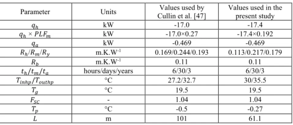
The present authors have also looked at the data for the Valencia case and determined the required borehole length based on their own interpretation of the data. Table 2 summarizes the results of these calculations and a comparison is made with the results provided by Cullin et al. [47]. As shown in Table 2, there are some significant differences in the evaluation of the parameters used in Equation 3.

First, the value of 𝑞𝑞_𝐶𝐶 is estimated to be -17.4 kW based on an analysis of the raw data. The 𝐶𝐶𝐿𝐿𝑃𝑃𝑚𝑚 value of 0.192 is

obtained from 2405/(17.4×720), where the value of 2405 kWh is the total heat injected during the 6th _{month of the third}

year of operation [47] and 720 is the number of hours in the month of June. Values of 𝑅𝑅ℎ, 𝑅𝑅𝑚𝑚, 𝑅𝑅𝑦𝑦 are also different. In

the present case, they are obtained using calculated values of the G-factor based on the solution of the ICS solution provided by Cooper [48] with a borehole radius of 75 mm, a thermal conductivity of 1.6 W/m-K [47], and a ground volumetric heat capacity of 2250 kJ/m3_{-K [46]. The values of 𝑇𝑇}

𝑖𝑖𝑛𝑛ℎ𝑝𝑝/𝑇𝑇𝑜𝑜𝑜𝑜𝑜𝑜ℎ𝑝𝑝 (30/35.5°C) are taken from the raw data at

the peak conditions. The calculated value of -0.27°C for 𝑇𝑇𝑝𝑝 is obtained using the original concentric ring technique

proposed by Kavanaugh and Rafferty [14] with a borehole separation distance of 3 m, a period of 3 years, and a borehole length of 61.1 m.

Table 2: Two different set of inputs to be used with the ASHRAE sizing equation for the Valencia case

Parameter Units _{Cullin et al. [47]} Values used by Values used in the _{present study}

𝑞𝑞ℎ kW -17.0 -17.4 𝑞𝑞ℎ × 𝐶𝐶𝐿𝐿𝑃𝑃𝑚𝑚 kW -17.0×0.27 -17.4×0.192 𝑞𝑞𝑎𝑎 kW -0.469 -0.469 𝑅𝑅ℎ/𝑅𝑅𝑚𝑚/𝑅𝑅𝑦𝑦 m.K.W-1 0.169/0.244/0.193 0.113/0.217/0.179 𝑅𝑅𝑏𝑏 m.K.W-1 0.11 0.11 𝑜𝑜ℎ/𝑜𝑜𝑚𝑚/𝑜𝑜𝑎𝑎 hours/days/years 6/30/3 6/30/3 𝑇𝑇𝑖𝑖𝑖𝑖ℎ𝑝𝑝/𝑇𝑇𝑜𝑜𝑜𝑜𝑜𝑜ℎ𝑝𝑝 °C 27.2/32.7 30/35.5 𝑇𝑇𝑔𝑔 °C 19.5 19.5 𝑃𝑃𝑆𝑆𝐶𝐶 - 1.04 1.04 𝑇𝑇𝑝𝑝 °C -0.5 -0.27 𝐿𝐿 m 101 61.1

The final calculated length (61.1 m) obtained using the ASHRAE sizing equation with the current set of inputs is much closer to the actual length (50 m) than the results of calculations performed by Cullin et al. [47] using the same ASHRAE sizing equation (100 m) but with a different set of inputs. If the duration of the peak heat load is assumed equal to 3

hours [49], the length obtained by the ASHRAE equation goes down to 56.8 m.These discrepancies show the importance

of human interpretation of the raw data on the final results. This is one reason why all loads are pre-treated in the inter-model comparison so that all tools have the same inputs. Li et al. [50] have also used the four cases introduced by Cullin

25

et al. [47] to validate their methodology which is based on a reformulation of the ASHRAE sizing equation. For the Valencia case presented in Table 2, they obtain a length of 77 m. Finally, as mentioned by Spitler [51], these four cases have reasonably balanced annual heat extraction and rejection loads with no significant long-term heat build-up or draw-down. Therefore, these data sets are not necessarily suited to check long-term effects.

4. Proposed test cases

One of the goals of this work is to propose a set of test cases that could be used to compare vertical GHE sizing tools against each other. With reference to the BESTEST terminology [52, 53] for building simulation software tools, three types of sizing test cases can be defined for comparisons: 1- simple analytical test cases, 2- comparative test cases and 3- real/experimental cases. Analytical test cases can only be applied for the simplest conditions (e.g. single borehole with constant load). Good long-term experimental data suitable for comparative testing could not be found in the literature. Therefore, only comparative test cases are examined in this work.

Differences in the required bore field length calculated by sizing tools can be the result of input errors or modeling differences. Input errors may be the results of human errors (e.g. different users may enter different ground thermal conductivities) or differences of interpretation for the raw data (e.g. different user may select different peak load duration or may convert building loads to ground loads differently). In an effort to avoid input errors, all test cases reported here are performed using a common set of data entered in each software by the same user and checked by another. Differences in results are thus presumed to be mainly due to the use of different modeling approaches or coding errors.

It should be noted that a spreadsheet containing all the loads and input data accompanies this paper so that other users can test other sizing tools with the same data. This spreadsheet also includes the test results of the inter-model comparison presented below. With reference to the general sizing equation (Equation 1), sizing tools will differ in the way they calculate the values of the ground thermal response, 𝑅𝑅𝑖𝑖, including in some cases the value of 𝑇𝑇𝑝𝑝, and the

borehole thermal resistance, 𝑅𝑅𝑏𝑏. Also, software tools from the same level will handle the summation term (in Equation

1) differently. In order to separate problems linked to the evaluation of 𝑅𝑅𝑏𝑏 from the rest of the calculation methodologies,

most of the test cases are solved with imposed values of 𝑅𝑅𝑏𝑏.

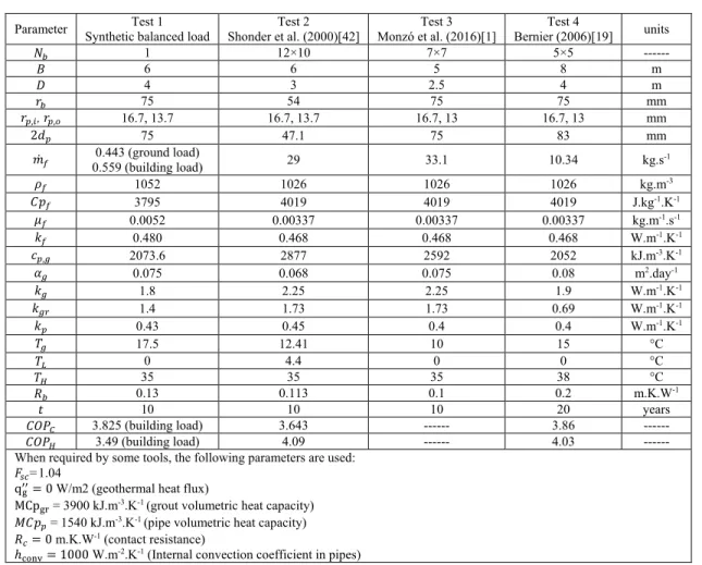
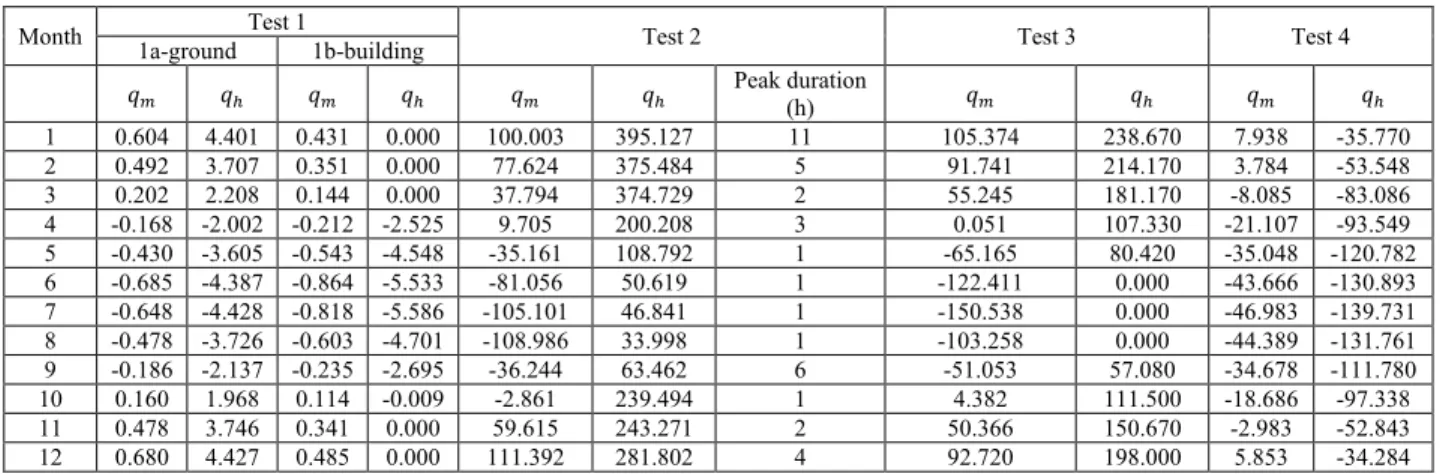
There are many data sets in the literature that could be used for inter-model comparative testing. A total of four data sets have been selected for the present study, each addressing a specific difficulty. A summary table of other data sets found

26

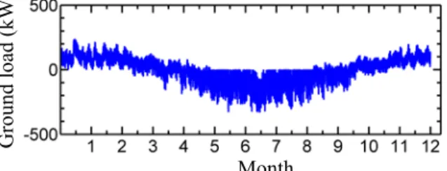
in the literature is provided in Appendix A. The four data sets include: i) a synthetic perfectly balanced hourly load profile; ii) the monthly and peak load data provided by Shonder et al. [42] for a school in Lincoln, Nebraska; iii) the set of monthly and peak load values presented by Monzó et al. [1]; iv) the hourly load profile used by Bernier [19] for a simulated building in Atlanta.

4.1. Input parameters

Table 3 shows the input parameters used for all test cases. Some tools need specific parameters that are not required by other tools. These parameters are listed at the bottom of Table 3.

Table 3: Input parameters for the four test cases

Parameter _{Synthetic balanced load} Test 1 _{Shonder et al. (2000)[42]} Test 2 _{Monzó et al. (2016)[1]} Test 3 _{Bernier (2006)[19]} Test 4 units

𝑁𝑁𝑏𝑏 1 12×10 7×7 5×5 --- 𝐵𝐵 6 6 5 8 m 𝐷𝐷 4 3 2.5 4 m 𝑟𝑟𝑏𝑏 75 54 75 75 mm 𝑟𝑟𝑝𝑝,𝑖𝑖, 𝑟𝑟𝑝𝑝,𝑜𝑜 16.7, 13.7 16.7, 13.7 16.7, 13 16.7, 13 mm 2𝑑𝑑𝑝𝑝 75 47.1 75 83 mm

𝑚𝑚̇𝑓𝑓 _{0.559 (building load)} 0.443 (ground load) 29 33.1 10.34 kg.s-1

𝜌𝜌𝑓𝑓 1052 1026 1026 1026 kg.m-3 𝑀𝑀𝑝𝑝𝑓𝑓 3795 4019 4019 4019 J.kg-1.K-1 𝜇𝜇𝑓𝑓 0.0052 0.00337 0.00337 0.00337 kg.m-1.s-1 𝑘𝑘𝑓𝑓 0.480 0.468 0.468 0.468 W.m-1.K-1 𝑠𝑠𝑝𝑝,𝑔𝑔 2073.6 2877 2592 2052 kJ.m-3.K-1 𝛼𝛼𝑔𝑔 0.075 0.068 0.075 0.08 m2.day-1 𝑘𝑘𝑔𝑔 1.8 2.25 2.25 1.9 W.m-1.K-1 𝑘𝑘𝑔𝑔𝑔𝑔 1.4 1.73 1.73 0.69 W.m-1.K-1 𝑘𝑘𝑝𝑝 0.43 0.45 0.4 0.4 W.m-1.K-1 𝑇𝑇𝑔𝑔 17.5 12.41 10 15 °C 𝑇𝑇𝐿𝐿 0 4.4 0 0 °C 𝑇𝑇𝐻𝐻 35 35 35 38 °C 𝑅𝑅𝑏𝑏 0.13 0.113 0.1 0.2 m.K.W-1 𝑜𝑜 10 10 10 20 years 𝑀𝑀𝐶𝐶𝐶𝐶𝐶𝐶 3.825 (building load) 3.643 --- 3.86 --- 𝑀𝑀𝐶𝐶𝐶𝐶𝐻𝐻 3.49 (building load) 4.09 --- 4.03 ---

When required by some tools, the following parameters are used: 𝑃𝑃𝑠𝑠𝑠𝑠=1.04

qg′′= 0 W/m2 (geothermal heat flux)

MCpgr = 3900 kJ.m-3.K-1 (grout volumetric heat capacity) 𝑀𝑀𝑀𝑀𝑝𝑝𝑝𝑝 = 1540 kJ.m-3.K-1 (pipe volumetric heat capacity) 𝑅𝑅𝑠𝑠= 0 m.K.W-1 (contact resistance)

ℎconv= 1000 W.m-2.K-1 (Internal convection coefficient in pipes)

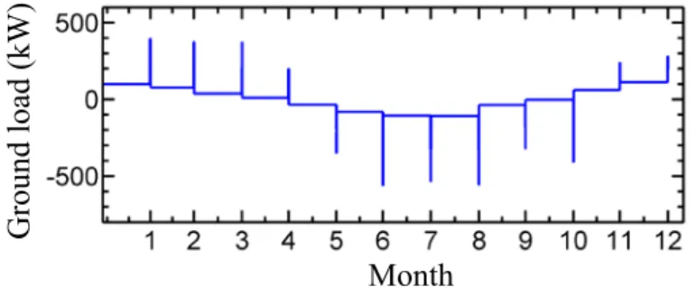
4.2. Test 1 -Synthetic balanced load – one borehole

The first test case uses a synthetically generated balanced load profile either as a ground load or as a building load. For this test, it is assumed that the load is handled by just one borehole. The sizing tools are compared on their ability to