HAL Id: hal-00875947
https://hal.inria.fr/hal-00875947
Submitted on 23 Oct 2013HAL is a multi-disciplinary open access archive for the deposit and dissemination of sci-entific research documents, whether they are pub-lished or not. The documents may come from
L’archive ouverte pluridisciplinaire HAL, est destinée au dépôt et à la diffusion de documents scientifiques de niveau recherche, publiés ou non, émanant des établissements d’enseignement et de
Chameleon: Customized Application-Specific
Consistency by means of Behavior Modeling
Houssem-Eddine Chihoub, María Pérez, Gabriel Antoniu, Luc Bougé
To cite this version:
Houssem-Eddine Chihoub, María Pérez, Gabriel Antoniu, Luc Bougé. Chameleon: Customized ApplicationSpecific Consistency by means of Behavior Modeling. [Research Report] INRIA Rennes -Bretagne Atlantique. 2013. �hal-00875947�
Chameleon: Customized Application-Specific
Consistency by means of Behavior Modeling
Houssem-Eddine Chihouba
, Maria S. Per`ezb
, Gabriel Antoniua
, Luc Boug´ec
a
INRIA Rennes-Bretagne Atlantique Rennes, France
b
Universidad Polit´echnica de Madrid Madrid, Spain
c
ENS Cachan-Antenne de Bretagne Bruz, France
Abstract
Multiple Big Data applications are being deployed worldwide to serve a very large number of clients nowadays. These applications vary in their perfor-mance and consistency requirements. Understanding such requirements at the storage system level is not possible. The high level semantics of an appli-cation are not exposed at the system level. In this context, the consequences of a stale read are not the same for all types of applications. In this work, we focus on managing consistency at the application level rather than at the system level. In order to achieve this goal, we propose an offline model-ing approach of the application access behavior that considers its high–level consistency semantics. Furthermore, every application state is automati-cally associated with a consistency policy. At runtime, we introduce the Chameleon approach that leverages the application model to provide a cus-tomized consistency specific to that application. Experimental evaluations show the high accuracy of our modeling approach exceeding 96% of correct classification of the application states. Moreover, our experiments conducted on Grid’5000 show that Chameleon adapts, for every time period, accord-ing to the application behavior and requirements while providaccord-ing best-effort performance.
Email addresses: [email protected](Houssem-Eddine Chihoub), [email protected](Maria S. Per`ez), [email protected] (Gabriel
1. Introduction
Recently, data sizes have been growing exponentially within many orga-nizations. In 2010, Eric Schmidt, the CEO of Google at the time, estimated the size of the World Wide Web at roughly 5 million terabytes of data [1] while the largest storage cluster within a corporation such as Facebook has more than 100 petabyte of Data in 2013 [2]. Data is everywhere and comes from multiple sources: social media, smart phones, sensors etc. This data tsunami, known as Big Data introduces multiple complications to the differ-ent aspects of data storage and managemdiffer-ent. These complications are due to the overwhelming sizes, but also the velocity required and the complexity of data coming from different sources with different requirements at a high load variability.
In order to deal with the related challenges, many Big Data systems rely on large and novel infrastructures, as well as new platforms and programming models. In this context, the emerging paradigm of Cloud Computing offers excellent means for Big Data. Within this paradigm, users can lease on-demand the computing and storage resources in Pay-As-You-Go manner with full support of elasticity. Therefore, corporations can acquire the resources needed for their Big Data applications at a low cost when needed. Meanwhile, they avoid large investments on physical infrastructures that need huge efforts for building and maintaining it, which, in addition, requires a high level of expertise.
Within cloud storage, replication is a very important feature for Big Data. At wide area cloud scales, and in order to deal with fast response and lo-cal availability requirements, data is replicated across multiple data centers. Clients therefore, can request data locally from a replica within the clos-est datacenter and get a fast response. Moreover, geographical replication provides data durability, fault tolerance and disaster recovery by duplicat-ing redundant data in different geographical areas. One issue that arises with replication however is guaranteeing data consistency across replicas. In this context, insuring strong consistency requires huge synchronization efforts across different locations and thus, exposes the users to the high net-work latencies. This affects the performance and the availability of the cloud storage solutions. One particular alternative that has become very popular is eventual consistency [3, 4]. Eventual consistency may tolerate inconsistency at some points in time but guarantees the convergence of all replicas to the same state at a future time.
The management of consistency impacts heavily storage systems. Fur-thermore, with Big Data scales, the management of consistency is critical matter to meet performance, availability, and monetary cost requirements. Traditional storage systems and databases that implement rigorous mod-els such as strong consistency have shown their limitations in meeting the scalability demands and the performance requirements of nowadays Big Data applications. In this context, flexible and adaptive consistency solutions that must consider the application requirements and provide only the adequate guarantees should be in the heart of the Big Data revolution.
Big Data Applications are different and so are their consistency require-ments. A web shop application for instance requires a stronger consistency as reading stale data could, in many cases, lead to serious consequences and a probable loss of client trust and/or money. A social network application on the other hand, requires a less strict consistency as reading stale data has less disastrous consequences. Understanding such requirements only at the level of the storage system is not possible. Both applications may impact the system state in the same manner at some points in time, for instance during holidays or high–sale seasons for the web shop and during important events for the social media. However, and while observing the same or similar stor-age system state, the consistency requirements can be completely different depending on the application semantics. In this work, and in contrast to related work, we focus on the application level with an aim at full automa-tion. We argue that in order to fully understand the applications and their consistency requirements, such a step is necessary. Moreover, automation is of extremely high importance given the large scales and the tremendous data volumes dealt with within today’s applications [2].
Many adaptive consistency models were proposed over the years such as our approach Harmony [5], and consistency rationing [6]. These approaches were mainly proposed in the purpose of dealing with dynamic workloads at the system level. They rely, commonly, on the data accesses observed in the storage system. Moreover, Harmony requires a small hint about consistency requirements (while consistency rationing focuses more on the cost of consis-tency violations). In contrast, we introduce Chamelon for a broader context —considering a wider range of workloads and consistency policies— to op-erate at the application level –instead of the system–. Chameleon therefore, identifies the behavior of the application (and subsequently identify when workloads exhibit dynamicity) in order to efficiently manage consistency.
level. Thereafter, when a dynamic policy such as Harmony is needed (for a given time period), the application tolerable stale rate can be computed automatically and communicated to the consistency policy (Harmony).
Chameleon, based on machine learning techniques, models the application and subsequently provides customized consistency specific to that applica-tion. The modeling is an offline process that consists in several steps. First, multiple predefined access pattern metrics are collected based on application past data access traces. These metrics are collected per time period. The chronological succession of time periods presents the application timeline. This timeline is further processed by machine learning techniques in order to identify the different states and states transitions of the application during its lifetime. Each state is then automatically associated with an adequate consistency policy from a broad class of consistency policies. The association is performed according to a set of specified input rules that reflect precisely the application semantics. Thereafter, based on the offline built model, we propose an online prediction algorithm that gives a prediction on the state and the associated consistency policy for the next time period of the appli-cation.
We have implemented the modeling approach in Java with extensive ex-perimental evaluations. We have used traces from Wikipedia as an illustra-tive large-scale application to show that our modeling achieves more than 96% of correct behavior recognition independently from the traces data used for training the classifier. We have implemented Chameleon in Java as well. For experimental evaluations, we have designed and implemented a bench-mark based on Wikipedia traces. We have deployed Chameleon with Cas-sandra as an underlying storage system on two remote sites on Grid’5000. We have demonstrated that Chameleon adapts, in each time period, to the specific consistency requirements of the application showing the eventual performance gains.
2. General Design 2.1. Design Goals
In order to build our approach, we set three major design goals that Chameleon must satisfy:
Automated application behavior understanding. In order to fully
to learn about its access behavior. The behavior of an application is responsible, in no small part, of defining the consistency needs. In gen-eral, the behavior of an application (such as Web services) changes over time periods and thus, expresses a degree of load variability. In this context, the behavior modeling of an application requires automation as it is extremely difficult for humans to perform such a task given the scales of today’s Big Data applications and the tremendous amount of information to process during their life cycles . Therefore, our target is to provide the two following automatized features: a robust behavior modeling of applications, and an online application behavior recogni-tion.
Application consistency semantics consideration. Understanding the
application behavior is necessary but not sufficient in order to behold the consistency requirements. The high-level consistency semantics of what the application need can only be provided by humans. For in-stance, defining what are the situations for which reading stale data is harmless or indicating whether update conflicts are managed (within the application or the storage system). In this context, these informa-tion are critical in order to provide the desirable level of consistency. Therefore, these application semantics should be provided in the form of rules that help associate every specific behavior of the application with a consistency policy. Hereafter, we propose mechanisms that make the task of rules setting and consideration simple and efficient.
Customized consistency specific to the application. A wide range of
Big Data applications are in production nowadays. These applications, generally, operate on very wide scales and have different behaviors as well as different consistency requirements. Therefore, our goal is to ex-ploit these differences by examining the application behavior in order to provide adequate consistency policy that is fully specific to the appli-cation. Such customized consistency allows the application to fulfill its target by providing the level of consistency required in every time pe-riod while optimizing SLA objectives such as performance, availability, economical cost, and energy consumption whenever it is possible. In this context, the application selects the most appropriate consistency policy whenever its current behavior changes.
2.2. Use Cases
Hereafter, we show few applications that express, in general, access be-havior variability (which is considered one of the main challenges of Big Data by SAS [7]). In this context, we show how these applications can, potentially, benefit from customized consistency.
Web Shop. A typical web shop that provides highly available services world wide exhibits high load variability. During the busy holidays periods (eg. christ-mas holidays), the underlying distributed storage or the database endures extremely heavy data accesses loads as the sales grow very high. Similarly, high loads are expected during discount periods. In contrast, the periods just after high–sale seasons are usually very slow resulting in very small number of data accesses at the storage system level. The system can experience an average load outside the aforementioned periods. Moreover, the data accesses may exhibit different patterns considering the level of contention to keys, the number of successive reads, the waiting time between two purchases of the same item etc. Our customized consistency approach, Chameleon, is designed for this purpose of access pattern (state) recognition in order to select the most pertinent consistency policy that satisfies the application requirements avoiding undesirable forms of inconsistency. A web shop’ one–year lifetime can be divided into 52 week-based time periods. Every time period exhibits an application state and is assigned a consistency policy specific to that state. Social Media. Social networks are typically worldwide services. Similar to Web shops, social media can exhibit high levels of load variability. High loads are expected during important events and breaking news (for general-purpose social networks for instance) while medium and low loads can be perceived when regular or no events are trending. Moreover, the load variability is location oriented. For instance, high loads –associated with a big event– that are perceived in one country will not be necessarily perceived in other locations. Therefore, data access patterns may vary in their loads but also in their behavior considering contention, locality and so many other criteria. Customized consistency can be applied for this type of applications to capture the states of the application in order to recognize access patterns and locality-based behavior. Accordingly, Chameleon selects adequately the consistency policy to adopt for a given time period. The application lifetime in this case can be a year long and a time period length equals one day for instance.
Wikipedia. Wikipedia is a collaborative editing worldwide–available service. While Wikipedia load variability is not comparable to the one of a web shop, it can still affect the consistency requirements. Moreover, the contention of accesses to the same keys is an important factor. Most of the time, con-tention is very low, mainly because of the large number of articles within Wikipedia covering a wide range of thematics. However, contention may change abruptly with articles becoming suddenly popular regarding their re-lation with recent breaking news or actuality events. Moreover, Wikipedia is a locality-based service. It is only normal that people would like to access ar-ticles written in their local languages (or the English language). Customized consistency can therefore, recognize the data access pattern in order to select the consistency policy considering Wikipedia tolerance for staleness. Stale-ness can be tolerated to a certain degree as reading a stale article means missing the last update to it, which is, in most times, not very important and consists of a line or small information addition. Therefore, Wikipedia service administrator can just specify an inconsistency window that should not be violated in order to preserve the desired quality of service. For in-stance, setting this window to one hour can be fairly acceptable. In this case, when a client reads an article it is guaranteed that it encapsulates all the updates that has been issued more than one hour ago.
2.3. Application Data Access Behavior Modeling
The first step towards customized consistency is to build an application model that express its different states and patterns in order to facilitate the task of apprehending its consistency requirements.
2.3.1. General Methodology
First, we introduce the global view of our methodology as to build an effi-cient application behavior modeling approach that must be automated with a high level of efficiency. The model will be leveraged in the next step as to provide insight into future consistency requirements of the application. The modeling phase starts with identifying different application states. Moreover, every state is associated with a consistency policy that is best fit. In addi-tion to state identificaaddi-tion, the model must specify the state transiaddi-tions of the application in order to reflect its lifetime behavior. The behavior modeling process requires the provision of past data access traces of an application as well as few of pre-defined rules in advance.
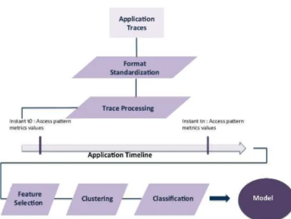
In the following, the different steps of the offline model construction, as shown in Figure 1, are presented. These steps are fully automated.
Application timeline construction. In this phase, application data traces
are processed in order to retrieve and compute a set of data access pat-tern metrics. These metrics are computed by specific time periods. The output of this phase is the application timeline where each time period of the timeline consists of a set of metric values. The appli-cation timeline refers to a an interval of time that characterizes the application.
Application states identification. After the construction of the
applica-tion timeline, all the time periods are processed using clustering tech-nique as to identify the different states exhibited by the application.
States classification. After the identification of the application states, an
offline learning process is performed. It consists in training a classifier based on the output dataset of the clustering technique. As a result of this phase, an online classifier that can recognize the application state or pattern at a given time period is built.
Consistency-State association. In this part, an algorithm that associates
with every application state a consistency policy is introduced. This algorithm relies on defined rules and application-specific parameters that reflect high level insight into the application consistency semantics. Consistency policies include strong and eventual consistency policies, static and dynamic policies, and local and geographical policies. The resulting model can be represented as a directed graph G(V, E) as shown in Figure 2 where vertices in V represent states and the edges in E represent the transitions that are chronological time successions as they are observed in the application timeline. The choice of a directed graph as a data structure facilitates the model storage providing efficient accesses to its different components. The computer representation of our model consists of an object that encapsulates the four following components:
The online classifier. This is the result of the states classifying phase.
This classifier is able to recognize the access pattern (the state) of the application for a given set of observed attributes.
First the timeline is constructed; then all time periods in the time-line are processed by unsupervised learning mechanisms for states identification; After states has been identified, states classification is performed.
Figure 1: Application modeling.
state1 state2 1 state4 4 state5 6 state3 2 3 5
State–Probability map. This map contains for every state identified its probability computed straightforwardly in the form of the occurrence number of the state by the number of occurrences of all states (number of time periods) fraction.
State–Policy map. This map is computed by the state-policy association
algorithm.
Transition set. This set contains all the transitions between states (as
de-fined by both the application timeline and states identification) with their respective ranks. The rank of a transition is its appearance order in the application model as it can be deduced from both the timeline and the results of states identification. An additional transition from the state of the last time period to the first is added with the highest rank.
2.3.2. Timeline Construction: Traces Processing
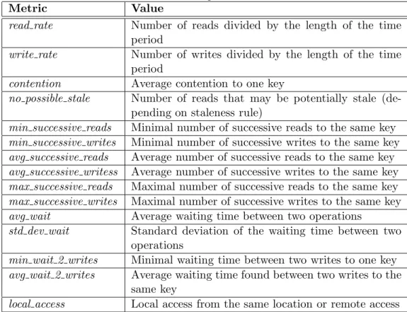
The application traces are converted to a standard formats in order to be processed by our approach. The traces are organized by time periods and every time period is stored in a specific file. Within every time period, metrics that exhibit the access pattern are extracted. These metrics are shown in Table 1 and express the behavior of the application when accessing data within the storage system.
These metrics characterize the access pattern and therefore, their values enable the capturing of the application state. This in turn, provides an insight into the consistency requirements. These metrics values are determinant to the states characterization, but to the consistency policy-state association as well. Metrics, such as the read rate, the write rate, and contention can help define the level of consistency strength needed. Similarly, the mean waiting time and the standard deviation of waiting time between two operations express the degree of dynamicity and variation exhibited by the application. On the other end, the minimal waiting time between two updates provides hints on the possibility of update conflicts.
At the end of this phase, the application timeline is built. It is composed of the chronological succession of time periods where every time period has specific access pattern metric values.
Table 1: Access pattern metrics.
Metric Value
read rate Number of reads divided by the length of the time period
write rate Number of writes divided by the length of the time period
contention Average contention to one key
no possible stale Number of reads that may be potentially stale (de-pending on staleness rule)
min successive reads Minimal number of successive reads to the same key min successive writes Minimal number of successive writes to the same key avg successive reads Average number of successive reads to the same key avg successive writess Average number of successive writes to the same key max successive reads Maximal number of successive reads to the same key max successive writes Maximal number of successive writes to the same key avg wait Average waiting time between two operations
std dev wait Standard deviation of the waiting time between two operations
min wait 2 writes Minimal waiting time between two writes to one key avg wait 2 writes Average waiting time found between two writes to the
same key
2.3.3. Identification of Application States
States identification is one of the critical tasks in the model building pro-cess. In order to achieve efficient states identification at large scale with full automation, we rely on machine learning techniques that are able to process large datasets with relatively large number of attributes. In this context, we construct a dataset from the application timeline. Every instance repre-sents a time period identified by a unique key, which is the timestamp of the period start. The access pattern metrics represent in this case the instance attributes. Our total number of attributes is 15. However, not all of these attributes may be relevant for all types of applications and therefore might affect badly the quality of both the supervised and unsupervised learning (ie. clustering and classification). In this context, we apply a feature selection algorithm that ranks the attributes in order of their relevance. Consequently, the unsupervised learning in the form of clustering is applied on the dataset with exclusively relevant features in order to identify the application different states.
Feature Selection. In machine learning, sample data is processed in order to extract knowledge that can be used for multiple aims. One of the most com-mon objectives is to use this knowledge in the purpose of making predictions about future data. In this context, the quality of the data sample used for training is critical to reach efficiency with learning algorithms. Feature selec-tion refers to the algorithms family that given the set of attributes selects a subset of relevant features and eliminates the irrelevant and redundant data that may make the knowledge discovery more difficult and cause overfitting problems [8].
In order to enhance the accuracy of our prediction model and avoid over-fitting, we use Recursive Feature Elimination (RFE ) [9, 10]. RFE best–fit use cases include small and average datasets with high dimensionality. There-fore, RFE is ideal for our model since considering our sample dimension and that the number of time periods in the application timeline is limited. RFE is, commonly, used with Support Vector Machines (SVM) and was originally applied to gene selection for cancer classification [9]. It helped scientists to discover novel information on genetics that was constantly missed in the past when using other techniques.
Data Clustering. In this context, clustering is applied to automatically iden-tify the application states. Multiple clustering algorithms exist. However, for
our model we seek an algorithm that requires minimal information from the user. In particular, we have no assumptions on the number of states (clus-ters), or their shapes that may be completely arbitrary. As a result, common algorithms such as k-means [11] or Gaussian Mixture EM clustering [12] show limitations over their applicability to our specific problem. Both algorithms can find only linearly separable clusters while the first one requires the num-ber of clusters in advance. However, at this stage we have minimal knowledge on the model and we do not put any assumptions during its construction. One clustering algorithm that fits our requirements is density-based spatial clustering of applications with noise DBSCAN algorithm [13]. We choose DBSCAN since it does not require the number of clusters but infers it implic-itly in the computation. Moreover, it can detect arbitrary shaped clusters.
DBSCAN is a density-based algorithm. Clusters are formed based on density reachability. Therefore, density variations are detected in order to form separated clusters of points. All points in the same cluster are mutually density reachable directly or by transitivity. DBSCAN requires two param-eters, the first one is the distance used to define density reachability, and the second one is the minimum points that a cluster should encapsulates. Defining the two parameters is known to be a difficult task in DBSCAN. In our model, the number of minimum points in a cluster is one since one time period in the application timeline may exhibit a state that is different from all other time periods. In contrast, defining a precise value of the distance parameter is more difficult. We plan to propose a heuristic that computes a near optimal value of this parameter as a future work.
2.3.4. State Classification
The next step in our model is to build an automated online classifier of application states. In order to provide such a feature, we use supervised machine learning techniques. The classifier utilizes a learning model that col-lects knowledge from an input sample offline in order to provide data analysis and patterns recognition abilities that will be used for instance classification. Based on the states identified in the previous step, a learning sample will be passed to the classifier. The learning sample consists of a set of time periods data, and for every time period its state. Multiple types of clas-sification techniques have been introduced. Two of the most efficient ones are Neural Networks [14] and Support Vectors Machines [15, 16]. Support Vector Machines (SVM) learning models were first introduced in 1992, and
most of statistical and learning techniques such as Neural Networks. In our model, we choose an SVM algorithm mainly because of its efficiency with high dimensionality data. Unlike Neural Networks, SVM techniques perform well with large datasets providing the necessary means to analyze data and find separations efficiently at high dimensionality. SVM represents data in a set of multidimensional space, then constructs a set of hyperplanes based on vectors in order to separate data points.
2.4. Rule-based Consistency-State Association
The process of identifying the application states lacks the consistency context. Therefore, states are identified based on access patterns that should be associated with the pertinent consistency policy based on the application semantics. In this part, we propose an algorithm that performs such an association.
2.4.1. Consistency Policies
Multiple consistency models were proposed over the years. Cloud storage systems usually implement a unique and well defined consistency model per system. However, in recent years multiple distributed storage systems that implement various models in order to provide different levels of consistency were introduced. Moreover, these systems provide flexible APIs to the client in order to select the consistency level on per operation basis.
In this work, we categorize a set of consistency policies considering the following properties:
• Strong policies vs. Eventual policies • Static policies vs. Dynamic policies • Local policies vs. Geographical policies
In this context, the following consistency policies are considered by the State–Policy association algorithm:
Strong Consistency. This is the static strong level of consistency by means
of synchronous replication involving all the replicas in read and write operations in order to avoid any form of inconsistency.
Eventual One Consistency. This is the basic level of static eventual con-sistency that involves only one replica —mainly the fastest replica to respond— in read and write operations.
Eventual Quorum Consistency. This policy is a static eventual policy.
The number of replicas involved in the access operations is equal to ⌊(number of replicas2 ) + 1⌋. Therefore, the fastest replicas to respond are
considered in this policy no matter their locations (eg. which data center, which rack etc.).
Eventual Local Quorum Consistency. In this static eventual local
pol-icy, only a quorum of replicas local to the accessed data center are considered in the read and write operations. Remote replicas (in other data centers ) are not solicited in order to avoid high network latencies between data centers.
Eventual Each Quorum Consistency. In contrast to the previous one,
this static eventual geographical policy considers local quorums in every data center for read and write operations.
Dynamic Performance Consistency. In this policy, the goal is to
dynam-ically tune the consistency level for dynamic workloads with a particu-lar focus on improving performance when possible. In our model, we use our approach Harmony, as the Dynamic Performance Consistency pol-icy. Subsequently, the tolerated stale read rate of an application is
com-puted automatically. Its value is equal to 100−undesirable stale reads
number of reads ×100
where the undesirable stale reads can be computed from the traces based on the input rules as it will be explained in the next section.
Dynamic Cost Consistency. This is a dynamic policy that adaptively
tunes the consistency level as well, with the goal of reducing the mon-etary cost of using the infrastructure (mainly cloud platforms) when possible. In our model, Bismar, introduced in Chapter 5, is the Dy-namic Cost Consistency.
Dynamic Energy Consistency. In this dynamic policy, the adaptive
se-lection of the consistency level must take into account the impact on energy consumption. In the absence of such a policy at the current time, we can either use Harmony or simply rely on the storage system
of future work, we plan on implementing a consistency policy where the main focus is to save energy when possible.
2.4.2. Input Rules
In order to reach a meaningful state-policy association, input information is required to be provided by the application administrator. Moreover, the administrator has the choice to either select one of the generic rules included in our model or implement its own specific rule based on its application semantics. These rules are used in the model to flag situations when staleness is not desired and may be harmful. Our model is provided with mainly two generic rules. The first rule is named the stock rule. It defines the number of the “consuming” updates to the same key per time period before flagging the successive reads as potentially reading undesirable values. This rule is based on the example of stock variables in web shop applications. As long as the value of such a variable is higher than a threshold value, the exact value of the variable is not required in order to avoid product availability conflicts that lead to anomalies. Therefore, stale data in this case is acceptable as it will not lead to the purchase of unavailable products. The second rule, surnamed the inconsistency window rule, is based on a provided inconsistency window value. The value of the inconsistency window is used later to compute the number of potential stale reads. In addition, for systems that are more tolerable for staleness, a second inconsistency window specific to the application is introduced. Its value is the maximum staleness interval that should not be exceeded. For instance, let consider the example of a social network where a given person friends should be able to read his updates that were committed more than given period of time ago (eg. two minutes ago). The stale reads that exceed this value are considered as undesirable (since they affect the quality of service for this case for instance). These two rules are provided in the following XML format:
<rules>
<allowed_staleness>
<type> stock or icw </type>
<stock> <min> 50 </min> </stock> <!-- or --> <inconsistency_window>
<native> storage_incon_window <native>
<tolerated> application_incon_window <tolerated> </inconsistency_window> <!-- or -->
</allowed_staleness> </rules>
Additional rules are necessary as well. A rule that specifies whether the update conflicts management is provided in the storage configuration or not is expected. If conflicts are not handled, any potential conflict situation would automatically lead to the application of the strong consistency policy. Moreover, the application administrator is required to specify whether dy-namic policies are allowed to be selected (if the specific conditions are met) or not. When dynamic policies are allowed, a variation threshold and the focus of the dynamic policy are required. The variation threshold will be compared to the standard deviation of waiting times and therefore, can be specified as α × mean waiting time where 0 < α < 1. These two rules are specified in the following XML format:
<rules>
<conflict_handling>
<flag> yes or no </flag> </conflict_handling>
<allow_dynamic>
<flag> yes or no </flag>
<variation_threshold> value </variation_threshold> <policy> performance or cost or energy </policy> </allow_dynamic>
</rules>
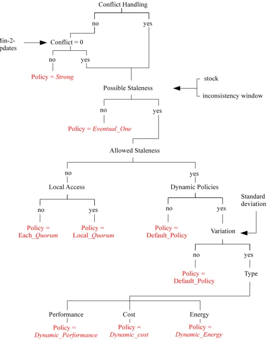
2.4.3. State-Consistency Association Algorithm
Figure 3 shows the state-policy association algorithm in a decision tree-like form. This is an offline algorithm. It takes as input the model with its identified states, the set of consistency policies, and the XML file with the input parameters and rules. For every state, the association algorithm aggregates metrics values from time periods that belong to that state. The algorithm starts by checking both the existence of update conflicts and mech-anisms to handle them in order to exclude or select the strong consistency policy. In the absence of conflicts, eventual quorum-based consistency levels can guarantee strong form of consistency. Therefore, the following step is to check the number of potential stale reads based on the provided staleness
one replica is selected or further processing is required. In the latter case, the algorithm checks whether staleness is allowed for the application. Sub-sequently, it selects Quorum-based levels if staleness is not allowed. The Local Quorum policy is chosen when accesses are potentially all or in–most directed to the local data center. In contrast, the Each Quorum policy is chosen for the non-local accesses (accesses to different data centers). On the other hand, if staleness is allowed, the algorithm checks whether dynamic policies are allowed as well. Hereafter, the dynamicity of the application workload is investigated based on the observed standard deviation of waiting times between data access operations. According to the variation threshold, the dynamic policy might be applied based on the desired optimization focus (ie. performance, cost, or energy consumption). In the case where dynamic policies are not allowed by the application administrator, a default policy is selected. Since in this case, staleness is allowed, we therefore choose the basic consistency level One as a default policy.
2.5. Prediction-Based Customized Consistency
After the offline model construction has been completed, we leverage the model as to provide customized consistency for the running application. Henceforth, we provide an online algorithm that at the end of every time period, and based on the model, gives a prediction on the expected state that the application should exhibit for the next time period. Accordingly, the consistency policy to adopt is chosen by a simple state-policy mapping. The prediction mechanisms are shown in Algorithm 1. The algorithm requires the application model and the current observed access pattern metrics (referred to as stats) collected from the application logs. The model consist of 4 components: the online state classifier, the State–Probability map, the State– Policy map, and the Transition set. The algorithm starts by classifying the current state of the application. Once the current state determined by the online classifier, its successor set in the application model is computed based on the transition set. In the case where this set is empty, the state with the highest probability is selected. If on the other hand, the set contains more than one successor, a recursive function recP rediction is called. This function leverages the model in order to provide insight into which state the application is expected to transform to.
The recursive function recP rediction checks the transitions of the ap-plication to the current state starting by the recent transition to the least
Algorithm 1: Next State Prediction. Input: Model, stats
Output: State
currentState← Model.Classif ier(stats)
if currentState successors set size = 0 then
nextState← def aultState
else
if currentState successors set size = 1 then
nextState← currentState successor
else
nextState← recP rediction(currentState,
predecessor(currentState), successors(currentState)) end
end
Function recPrediction(state1, state2, successors)
M ax← random state in successors
tr← T ransition(state2, state1) rank
for state in successors do if state rank < tr then
successors ← successors − {state}
if State Probability > Max Probability then
M ax← State
end
if successors set size > 1 and predecessor(state2) != ∅ then return
recP rediction(state2, predecessor(state2), successors) else
if successors set size = 0 or predecessor(state2) = ∅ then
return M ax
else
return the successor in successors
end end end
or conserved based on their ranks. Therefore, only states that are expected after the succession of the states exhibited so far are not ruled out. The recursive call traces the transitions from the recent to the old one until no or only one state belongs to the successors set. In the case where the successor set is not empty nor include only one element while the oldest transition has been reached, the state with the highest probability is selected.
3. Implementation and Experimental Evaluations
In this section, we first describe the implementation of Chameleon. Sec-ondly, we present our experimental evaluation. The main goal is to demon-strate the quality of the modeling behavior approach and to show the ef-ficiency of Chameleon in adapting to the need of the application at full automation, which is the goal we were seeking when designing it. In this context, the recognition of the application behavior and its requirements is performed by the online classifier (SVM), which is a black box to the human users.
3.1. Implementation
Chameleon targets a wide range of large-scale applications. These appli-cations might be completely different. Moreover, their traces are potentially heterogeneous in both content and formats. In order to deal with such a heterogeneity, Chameleon is designed to easily integrate new data formats and to automatically deal with data variability. Chameleon implementation is divided into two main parts: the traces parsing part, and the modeling and the online prediction part.
Traces parsing and timeline construction. At the start of this phase, the application traces (logs) are converted into a standard format. We define the standard format where each line consists of the following values separated by one blank: timestamp of the operation, the key of accessed data, the type of access operation, and, if possible to get this information, a flag to indicate whether the geo–location of the client is local or not. This approach makes the integration of any new application (and its traces) easy by just writing the corresponding converter to the standard format. The traces in the standard format are processed by a Python built module. This module divides the large traces log file into time periods based on the timestamps and then
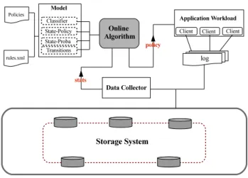
Figure 4: Overview of Chameleon Implementation
is loaded at a time from the disk and then processed in order to efficiently use memory space. Hereafter, all computed metrics values of each time period are stored in one file that represents the application timeline.
Modeling and online prediction. The second part of Chameleon implementa-tion builds the applicaimplementa-tion model and the online predicimplementa-tion algorithm. This part is implemented in Java where the application model is an object. Fig-ure 4 shows our implementation. The model component encapsulates the model data. The model is instantiated before runtime based on the appli-cation timeline, the input rules file, and the set of consistency policies. At runtime, every application client logs its access information. The data col-lector component collects the necessary data from client logs and extracts the data access statistics to be send to the online algorithm component. The latter uses the knowledge acquired from the model component in order to perform the prediction computations of the next consistency policy to use during the next time period. The machine learning algorithms applied for state identification and classification were implemented based on the Java Machine Learning Library (Java–ML) [17]. Java–ML wraps over multiple other machine learning libraries in Java. The recursive feature elimination RFE implementation was Java–ML native while the clustering algorithm was wrapped over the DBSCAN implementation in Weka library [18] and the classification algorithm was wrapped over SVM in LIBSVM library [19].
0 20 40 60 80 100 120 0 0.2 0.4 0.6 0.8 1 number of clusters distance parameter DBSCAN with RFE DBSCAN without RFE number of time periods
(a) Clustering performance
0 20 40 60 80 100 120 0 0.2 0.4 0.6 0.8 1 1.2
prediction success rate (%)
distance parameter classification with RFE classification without RFE
(b) Classification accuracy Figure 5: DBSCAN Clustering evaluation with and without RFE
3.2. Model Evaluation: Clustering and Classification
Wikipedia Traces. In order to validate our modeling phase, we investigated available traces of large-scale applications that fit our case study. A perfect use-case match is Wikipedia [20]. Based on access traces collection and analysis of Wikipedia described in [21], we use a traces sample collected in 1st of January 2008. The traces consisted of roughly 9056528 operation and a total log file size of approximately 1 GB. The access traces consisted of the timestamp of the operation occurrence, the page that was accessed, and the type of the operation. Unfortunately, the information related to the client geographical location was not available. These traces were processed to extract relevant metrics (as described in the modeling section) and construct the application timeline in order to perform experimental evaluations. For the purpose of experimental evaluation, the length of a time period is set to 100 seconds and the application timeline consists of 90 time periods.
Setup. The experimental sets to evaluate the offline modeling phase were conducted on a Mac equipped with Intel-Core-2-Duo CPU of 2,66 GHz fre-quency, memory size of 4 GB and a 300 GB hard drive. The used operating system is Mac OS X 10.6. The Java Runtime Environment version was 1.6. Clustering Evaluation. In order to validate our model, we ran a set of ex-periments oriented to evaluate the performance of the clustering algorithm DBSCAN used for states identification as well as the quality of classification. We first start by analyzing the DBSCAN algorithm and its behavior when
the minimal number of points that a cluster should enclose has been fixed to one (as one application time period can exhibit a behavior different from all others). Moreover, we compare the numbers of found clusters every time with and without recursive feature elimination RFE. Figure 5(a) shows the varying number of the formed clusters when varying the distance parameter in the interval 0.10 to 1.05 for the Wikipedia sample timeline. The number of clusters increases when decreasing the value of the distance parameter. The two clustering approaches with and without RFE find a close number of clusters which shows that the application of RFE preserves the intuitive clustering results of DBSCAN while enhancing greatly the quality of classi-fication as it will be demonstrated. With the very small distance parameter value of 0.10, the number of found clusters for both approaches equals that of the number of time periods (data instances). This makes the clustering in-effective and the classification phase more difficult. Similarly, with the value of 1.05, the found number of clusters is one for both approaches making the whole modeling process trivial. Moreover, We can observe that with small distance parameter values, the clustering approach that is not preceded with RFE forms more clusters. This is mainly, because of the recursive and trivial features not being eliminated. In addition, these features (attributes) will affect badly the classification quality.
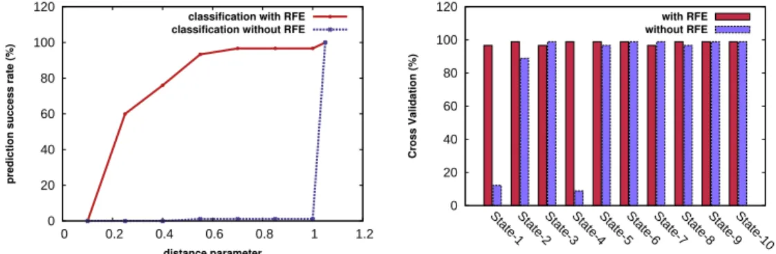
In order to analyze the impact of the two clustering approaches (with and without RFE) on the classification process, we train our SVM algorithm with the clustered output data of both approaches. After that, we classify every data instance in the Wikipedia timeline with the two classifiers (with and without applying RFE). Subsequently, we compare the predicted value by the classifier with the observed value from the clustering phase in order to determine the prediction success rate. Figure 5(b) clearly and conclusively shows the importance of the recursive feature elimination in the classification process. Clustering and classification without RFE results in a very mediocre classifier with very small fractions of successful predictions. In contrast, RFE makes the whole process very effective with 100% fraction of successful predictions on the training data. However, the classifier in this latter case might suffer from the overfitting to the data sample and may behave badly with outsider (new coming) data instances. Therefore, we conduct a set of experiments hereafter to evaluate the classification quality independently to the input dataset.
0 20 40 60 80 100 120 0 0.2 0.4 0.6 0.8 1 1.2
prediction success rate (%)
distance parameter classification with RFE classification without RFE
(a) Classification of new data instances: ac-curacy 0 20 40 60 80 100 120 State-1State-2State-3State-4State-5State-6State-7State-8State-9State-10 Cross Validation (%) with RFE without RFE
(b) Cross–Validation of classification with different states
Figure 6: Croos–Validation
Cross–Validation. Recursive feature elimination RFE algorithm was applied mainly to enhance the quality of the classification. In order to evaluate the classification algorithm and to check whether it suffers from the over-fitting problem, we ran a cross–validation evaluation. We divide the data resulting from the clustering phase into two sets. The first set that contains randomly selected fraction of two thirds of data instances used to train the classifier. The second set contains the remaining data and is used for clas-sification. Figure 6(a) shows the prediction success rate of both approaches with and without RFE where the classified data is different from the training data. As expected, the classifier without RFE performs extremely bad with very low, sometimes null, prediction success rates. In contrast, RFE–SVM classifier achieves very high success rates (over 96%) when the distance pa-rameter value is greater than 0.55. Moreover, it performs reasonably well with relatively small distance values such as 0.25 (over 56% success rate). However, the classification proved ineffective with a distance of 0.10. The reason for such a behavior is the inefficiency of the clustering algorithm with this distance value since all data instances are classified in distinct classes. As part of a future plan, we intend to investigate the possibility of a heuris-tic that targets the computation of the distance value. Such a heurisheuris-tic should aim at computing a value that provides high success rate while re-sulting in a number of clusters higher than a given number (for instance
α× number of consistency policies).
ap-plication –observed in the data sample– when the distance parameter in the clustering phase equals 0.55. The cross–validation type used is K-fold cross-validation with k equals to 10. The 90 time periods (instances) were classified correctly for the big majority of states of the classification with RFE (Over 96% successfully classified for all states) which shows the robustness and the precision of our model that is data set–independent. In contrast, classifi-cation without RFE classifies instances at very low accuracy for few states and at high accuracy rates for others. However, the poor success rate shown in Figure 6(a) is caused essentially by the poor classification with states 1 and 4. In particular, because the number of time periods that exhibits these two states is significantly higher than others. Moreover, the successful cross-validation with other states is, mainly, because of true negatives rather than true positives.
3.3. Customized Consistency: Evaluation
Experimental Setup. We ran the experiment sets to evaluate the online model on Grid’5000 [22]. We used Cassandra [23] as a hosting storage system. Therefore, we deployed Cassandra-1.2.3 [24] version on two sites on Grid’5000 with 3 replicas in each site. 30 nodes were deployed on Sophia and 20 nodes on Nancy. Nodes in Sophia are equipped with 300 GB hard drives, 32 GB of memory, and 2-CPUs 8-cores Intel Xeon. The Nancy nodes are equipped with disks of 320 GB total size, 16 GB of memory, and 2-CPUs 8-cores Intel Xeon. In addition, the network connection between the two sites in the south and the north east of France is provided by Renater (The French national telecommunication network for technology, education, and research). At the time of running the experiment sets, the average round trip latency between the two sites was roughly 18.53 ms.
Micro–Benchmark. We designed a micro–benchmark that exhibits the same characteristics shown in the used Wikipedia traces. It was extremely difficult to reproduce exactly the same or closely similar behavior. The main challenge is that we do not have enough resources (with our 50–nodes Cassandra cluster and network speed) to reproduces the same extremely high throughput and small waiting times between operations exhibited in the traces. Therefore, we designed a micro-benchmark that keep Wikipedia load characteristics with amplified waiting times between operations. The designed workload is implemented in Java and divided into 90 time periods (the number of time periods computed from Wikipedia traces). Every time period consists of
0 20 40 60 80 100 STATE-1STATE-2STATE-3STATE-4STATE-5STATE-6STATE-7STATE-8 Probability (%) Clustering Online prediction
Figure 7: Observed states distribution
specific properties: read rate, write rate, contention to the same keys, and average waiting time between operations values. These values are computed directly from the Wikipedia traces (with amplified waiting times) and saved into a configuration file. At runtime, the waiting time between operations is generated randomly following an exponential distribution where the mean equals the average waiting time. In order to run the online model evaluation, we first run the benchmark to generate new traces that will be used for offline model construction.
Online Prediction. In order to run Chameleon, we have selected the inconsis-tency window rule as an input rule to apply with Wikipedia. For the purpose of experimental evaluation and given our experiment scale, we assume that the tolerated stale reads are the ones that enclose updates older than one minute (60000 ms). Moreover, we consider that updates conflicts are man-ageable since it is possible to solve them at a latter time by Cassandra based on causal ordering (Anti–Entropy operation). We consider in addition, that dynamic policies are allowed with a focus on performance. The variation threshold value is fixed at 25% of the mean waiting time.
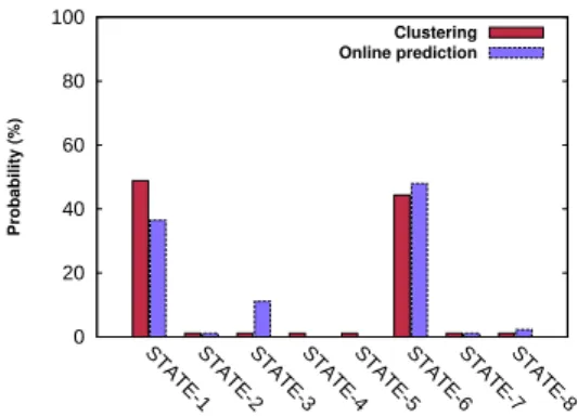
Figure 7 shows the probability of observing the different states. We com-pare the probability of states observed from past access traces by means of clustering and the probability of predicted states at runtime. The results clearly show that for the states with the highest probabilities (mainly State-1 and state-6) the probability is closely similar, which demonstrates the effi-ciency of our online prediction model in predicting similar behavior to the one modeled. We can observe that for State-3 the probability at runtime is
0 10 20 30 40 50 60 70 80 90 0 10 20 30 40 50 60 70 80 90 latency (ms) time periods Eventual One Chameleon Eventual Quorum Strong
(a) Latency evaluation
0 50 100 150 200 250 300 350 400 0 10 20 30 40 50 60 70 80 90 throughput (op/s) time periods Eventual One Chameleon Eventual Quorum Strong (b) Throughput evaluation Figure 8: Performance Evaluation of Chameleon
that can be associated with classification, the random generation of wait-ing times in the workload, as well as the the performance of the Cassandra storage system (that might be slightly affected in particular by events and traffic on the shared network) and might therefore, affects slightly the load characteristics.
Latency and Throughput. Figure 8(a) and Figure 8(b) show the performance exhibited by our approach Chameleon in comparison to different consistency policies. In Figure 8(a), we can observe that both the Quorum and Strong static consistency policies result in a high operation latencies throughout the different time periods of the workload. Such high latencies are mainly be-cause these policies suffer from high wide–area network latency. In contrast, the eventual One policy achieves the lowest operation latencies since data are accessed from closest local replicas. However, with this policy, multiple consistency violations might occur. Our approach, Chameleon, shows a high latency variability across the different time periods while the latency is rel-atively low and close to the lowest one most of the time. This variability is the result of adapting the consistency policy according to the application behavior exhibited in that specific time period. Therefore, Chameleon pro-vides specifically a consistency policy in accordance to the application state for every time period.
Similarly, Figure 8(b) shows the throughput of the different consistency policies throughout the workload time periods. Both the Quorum and the strong policies show relatively low throughputs. The throughput in these cases suffers from the wide area network latency as well as the extra traffic
0 10 20 30 40 50 0 10 20 30 40 50 60 70 80 90
Number of stale reads
time periods Eventual One
Chameleon Eventual Quorum Strong
Figure 9: Data staleness evaluation
in the network generated by these consistency policies. This can be in partic-ular penalizing for a highly on-demand service such as Wikipedia. The One policy on the other hand, exhibit much higher throughput but, at the cost of potentially consistency violations. Chameleon shows variable throughput (similar to latency) that depends on the behavior of the application in the given time period. Therefore, the consistency policy is selected to suit that behavior of the application. Although, a high level of variability is observed, Chameleon throughput is almost always better than the Quorum’s and rel-atively close to the throughput of the One policy.
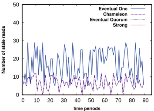
Data Staleness. After the investigation of the different consistency policies, we show in Figure 9 the staleness of data throughout the workload timeline. The Quorum and the Strong policies provide high levels of consistency with no stale data being read. However, this comes at the cost of lower perfor-mance and availability, in particular if we consider that staleness is both rare (because of the low contention to data) and is accepted to a certain degree within Wikipedia. The One level allows the highest number of stale data, though these numbers are relatively small since the contention of data ac-cesses to the same keys is not high. Moreover, the One policy might allow undesirable forms of staleness (eg. reading very old data). Chameleon allows for very small number of reads to be stale. Moreover, these stale reads are expected in accordance with the specified rules during the state–consistency association phase. Therefore, tolerating such a small “unharmfull” fractions of stale reads comes with huge benefits for performance support, money sav-ings, or energy consumption reduction.
4. Related Work
Using past data access traces in the purpose of studying consistency was investigated in [25]. Anderson et al. proposed mechanisms that process past accesses traces offline in order to check few consistency guarantees and whether they were violated or not during runtime. The main purpose of this work is the analysis and the validation of the past execution of a workload in order to understand the provided consistency guarantees of a key–value store. One of their primary observations is that consistency violations are correlated with the increasing contention of operations to the same keys.
Few adaptive consistency models were proposed over the years [6, 26, 27, 28]. Most of these approaches focus on consistency management on the storage system level. Therefore, there is a little or no focus on consistency requirements on the applications side. Moreover, no extensive study of the application data access behavior was introduced. In [27], the authors propose a flexible consistency model that variates the level of guarantees depending on the nature of operation executed in relation with the application semantic. However, the selection of consistency level of one operation is not automatic and may be very difficult to induce by application developers, in particular with today’ scales. Kraska et al. [6] propose an approach that imposes the consistency level on data instead of transactions. Therefore, data is divided into three categories depending on the consistency guarantees to be provided. The main difficulty with this approach is the lack of automation when cate-gorizing the data, which may be in our case of Big Data applications a huge obstacle, since the administrator is required to categorize huge volumes of potentially heterogenous data manually. Both approaches in [26, 28] do not consider the application requirements as the first approach takes into consid-eration only the read rates and the write rates with no application semantics consideration while the second approach was proposed in the particular con-text of providing persistent storage to databases in the cloud.
Multiple works contributed to the area of modeling and characterizing
large-scale infrastructures and applications. Montes et al. [29] proposed
GloBeM a global behavior modeling for the whole grid. GloBeM rely on machine learning and knowledge discovery techniques in order to represent the different sub-systems of the grid into one global model in the form of finite state machine. This model allows the system administrators to predict future grid state transitions and therefore anticipate any undesirable states. Other works focused on the characterization and analysis of large-scale application
workloads and their behaviors. In [21], the authors study Wikipedia access traces and accordingly classify client requests and collect access metrics such as the number of read and save operations, and load variations. In a differ-ent work [30], the authors study the user behavior in online social networks. They propose a thorough analysis of social network workloads with regard to the user behavior in an attempt to enhance the interface design, provide better understanding of social interactions, and improve the design of con-tent distribution systems. However, none of these studies were leveraged as to provide a vision on consistency management.
5. Conclusion
Consistency management in large–scale storage systems has been widely studied. Most of existing work focused on leveraging consistency tradeoffs and the impacts on the storage system with a secondary minimal focus on the application consistency requirements. In this paper, we focus instead on the applications in order to fully apprehend their consistency requirements. Therefore, we first introduce an automatized behavior modeling approach that detects the different states of an application lifecycle. These states are thereafter associated with adequate consistency policies based on the application semantics. The application model is leveraged in a second step as to provide a customized consistency specific to the application. At runtime, our approach, Chameleon, identifies the application state by means of efficient classification techniques. Accordingly it provides a prediction on the behavior of the application and subsequently selects the best-fit consistency policy for the following time period. Experimental evaluation have shown the efficiency of our modeling approach where the application states are identified and predicted with a success rate that exceeds 96%. Moreover, we have shown how our approach Chameleon is able to adapt specifically to the application behavior at every time period in order to provide the desired properties (including performance, cost, and energy consumption) with no undesirable consistency violations.
References
[1] 5 million terabytes of data (March 2013).
[2] Under the Hood: Scheduling MapReduce jobs more efficiently with Corona (April 2013).
URL https://www.facebook.com/notes/facebook-engineering/
under-the-hood-scheduling-mapreduce-jobs-more-efficiently-with-corona/10151142560538920
[3] M. Shapiro, B. Kemme, Eventual Consistency, in: M. T. ´Ozsu, L. Liu (Eds.), Encyclopedia of Database Systems (online and print), springer, 2009.
[4] W. Vogels, Eventually consistent, Commun. ACM (2009) 40–44.
[5] H.-E. Chihoub, S. Ibrahim, G. Antoniu, M. S. P´erez-Hern´andez, Harmony: Towards automated self-adaptive consistency in cloud storage, in: 2012 IEEE International Conference on Cluster Computing (CLUSTER’12), Beijing, China, 2012, pp. 293–301.
[6] T. Kraska, M. Hentschel, G. Alonso, D. Kossmann, Consistency rationing in the cloud: pay only when it matters, Proc. VLDB Endow. 2 (2009) 253–264. [7] Big Data What Is It? (April 2013).
URL http://www.sas.com/big-data/
[8] J. Weston, A. Elisseeff, B. Schlkopf, P. Kaelbling, Use of the zero-norm with linear models and kernel methods, Journal of Machine Learning Research 3 (2003) 1439–1461.
[9] I. Guyon, J. Weston, S. Barnhill, V. Vapnik, Gene selection for cancer classifi-cation using support vector machines, Mach. Learn. 46 (1-3) (2002) 389–422. [10] X. wen Chen, J. C. Jeong, Enhanced recursive feature elimination, in: Sixth International Conference on Machine Learning and Applications, 2007. ICMLA 2007., 2007, pp. 429–435.
[11] J. B. MacQueen, Some methods for classification and analysis of multivariate observations, in: L. M. L. Cam, J. Neyman (Eds.), Proc. of the fifth Berkeley Symposium on Mathematical Statistics and Probability, Vol. 1, University of California Press, 1967, pp. 281–297.
[12] A. P. Dempster, N. M. Laird, D. B. Rubin, Maximum likelihood from incom-plete data via the em algorithm, JOURNAL OF THE ROYAL STATISTICAL SOCIETY, SERIES B 39 (1) (1977) 1–38.
[13] M. Ester, H. peter Kriegel, J. S, X. Xu, A density-based algorithm for discov-ering clusters in large spatial databases with noise, in: Second International Conference on Knowledge Discovery and Data Mining, AAAI Press, 1996, pp. 226–231.
[14] W. S. McCulloch, W. Pitts, Neurocomputing: foundations of research, MIT Press, 1988, Ch. A logical calculus of the ideas immanent in nervous activity, pp. 15–27.
[15] B. E. Boser, I. M. Guyon, V. N. Vapnik, A training algorithm for optimal mar-gin classifiers, in: Proceedings of the fifth annual workshop on Computational learning theory, COLT ’92, ACM, 1992, pp. 144–152.
[16] C. Cortes, V. Vapnik, Support-vector networks, Mach. Learn. 20 (3) (1995) 273–297.
[17] Java machine learning library (java-ml) (July 2013). URL http://java-ml.sourceforge.net/
[18] Weka 3: Data mining software in java (July 2013). URL http://www.cs.waikato.ac.nz/ml/weka/
[19] Libsvm – a library for support vector machines (July 2013). URL http://www.csie.ntu.edu.tw/ cjlin/libsvm/ [20] Wikipedia (July 2013).
URL http://en.wikipedia.org/
[21] G. Urdaneta, G. Pierre, M. van Steen, Wikipedia workload analysis for de-centralized hosting, Elsevier Computer Networks 53 (11) (2009) 1830–1845. URL http://www.globule.org/publi/WWADH comnet2009.html
[22] Y. J´egou, S. Lant´eri, J. Leduc, et al., Grid’5000: a large scale and highly reconfigurable experimental grid testbed., Intl. Journal of High Performance Comp. Applications 20 (4) (2006) 481–494.
[23] A. Lakshman, P. Malik, Cassandra: a decentralized structured storage sys-tem, SIGOPS Oper. Syst. Rev. 44 (2010) 35–40.
[24] Apache Cassandra (February 2013). URL http://cassandra.apache.org/
[25] E. Anderson, X. Li, M. A. Shah, J. Tucek, J. J. Wylie, What consistency does your key-value store actually provide?, in: Proceedings of the Sixth international conference on Hot topics in system dependability, HotDep’10, USENIX Association, Berkeley, CA, USA, 2010, pp. 1–16.
[26] X. Wang, S. Yang, S. Wang, X. Niu, J. Xu, An application-based adaptive replica consistency for cloud storage, in: Grid and Cooperative Computing (GCC), 2010 9th International Conference on, 2010, pp. 13 –17.
[27] C. Li, D. Porto, A. Clement, J. Gehrke, N. Pregui¸ca, R. Rodrigues, Making geo-replicated systems fast as possible, consistent when necessary, in: Pro-ceedings of the 10th USENIX conference on Operating Systems Design and Implementation, OSDI’12, USENIX Association, 2012, pp. 265–278.
[28] R. Liu, A. Aboulnaga, K. Salem, Dax: a widely distributed multitenant stor-age service for dbms hosting, in: Proceedings of the 39th international con-ference on Very Large Data Bases, PVLDB’13, VLDB Endowment, 2013, pp. 253–264.
[29] J. Montes, A. Snchez, J. J. Valds, M. S. Prez, P. Herrero, Finding order in chaos: a behavior model of the whole grid, Concurrency and Computation: Practice and Experience 22 (11) (2010) 1386–1415.
[30] F. Benevenuto, T. Rodrigues, M. Cha, V. Almeida, Characterizing user be-havior in online social networks, in: Proceedings of the 9th ACM SIGCOMM conference on Internet measurement conference, IMC ’09, ACM, 2009, pp. 49–62.