HAL Id: insu-02179077
https://hal-insu.archives-ouvertes.fr/insu-02179077
Submitted on 20 Sep 2019
HAL is a multi-disciplinary open access
archive for the deposit and dissemination of
sci-entific research documents, whether they are
pub-lished or not. The documents may come from
teaching and research institutions in France or
abroad, or from public or private research centers.
L’archive ouverte pluridisciplinaire HAL, est
destinée au dépôt et à la diffusion de documents
scientifiques de niveau recherche, publiés ou non,
émanant des établissements d’enseignement et de
recherche français ou étrangers, des laboratoires
publics ou privés.
R. Janssen, A. Tsimpidi, A. Karydis, A. Pozzer, J. Lelieveld, M. Crippa, A.
Prévôt, W. Ait-Helal, A. Borbon, S. Sauvage, et al.
To cite this version:
R. Janssen, A. Tsimpidi, A. Karydis, A. Pozzer, J. Lelieveld, et al.. Influence of local production
and vertical transport on the organic aerosol budget over Paris. Journal of Geophysical Research:
Atmospheres, American Geophysical Union, 2017, 122 (15), pp.8276-8296. �10.1002/2016JD026402�.
�insu-02179077�
Influence of local production and vertical
transport on the organic aerosol
budget over Paris
R. H. H. Janssen1,2 , A. P. Tsimpidi1, V. A. Karydis1, A. Pozzer1 , J. Lelieveld1, M. Crippa3,4 ,
A. S. H. Prévôt3 , W. Ait-Helal5,6,7, A. Borbon6 ,S. Sauvage5, and N. Locoge5
1Atmospheric Chemistry Department, Max Planck Institute for Chemistry, Mainz, Germany,2Department of Civil and Environmental Engineering, Massachusetts Institute of Technology, Cambridge, Massachusetts, USA,3Laboratory of Atmospheric Chemistry, Paul Scherrer Institute, PSI Villigen, Switzerland,4Now at Directorate for Energy, Transport and Climate, Air and Climate Unit, Joint Research Centre (JRC), European Commission, Ispra, Italy,5Mines Douai, SAGE, Douai, France,6LISA, UMR CNRS 7583, Université Paris Est Créteil et Université Paris Diderot, Institut Pierre Simon Laplace, Créteil, France,7Now at Institut de Combustion, Aérothermique, Réactivité et Environnement (ICARE), CNRS (UPR 3021)/OSUC, Orléans, France
Abstract
We performed a case study of the organic aerosol (OA) budget during the MEGAPOLI campaign during summer 2009 in Paris. We combined aerosol mass spectrometer, gas phase chemistry, and atmospheric boundary layer (ABL) data and applied the MXL/MESSy column model. We find that during daytime, vertical mixing due to ABL growth has opposing effects on secondary organic aerosol (SOA) and primary organic aerosol (POA) concentrations. POA concentrations are mainly governed by dilution due to boundary layer expansion and transport of POA-depleted air from aloft, while SOA concentrations are enhanced by entrainment of SOA-rich air from the residual layer (RL). Further, local emissions and photochemical production control the diurnal cycle of SOA. SOA from intermediate volatility organic compounds constitutes about half of the locally formed SOA mass. Other processes that previously have been shown to influence the urban OA budget, such as aging of semivolatile and intermediate volatility organic compounds (S/IVOC), dry deposition of S/IVOCs, and IVOC emissions, are found to have minor influences on OA. Our model results show that the modern carbon content of the OA is driven by vertical and long-range transport, with a minor contribution from local cooking emissions. SOA from regional sources and resulting from aging and long-lived precursors can lead to high SOA concentrations above the ABL, which can strongly influence ground-based observations through downward transport. Sensitivity analysis shows that modeled SOA concentrations in the ABL are equally sensitive to ABL dynamics as to SOA concentrations transported from the RL.1. Introduction
In spite of rapid developments in our understanding of organic aerosol (OA) physicochemical properties, representing the composition and evolution of OA in models over urban areas remains to be a challenge [e.g., Volkamer et al., 2006; Zhang et al., 2007; Dzepina et al., 2009; Jimenez et al., 2009; Zhang et al., 2013; Tsimpidi
et al., 2016]. Measurements during campaigns in various megacities have helped to gain insight in processes
that govern OA. In addition, modeling can help in analyzing the measurements and to break down the observed signal into the contributions of the underlying processes. Several modeling studies have addressed the influence of individual processes on the OA budget in urban areas. Robinson et al. [2007], Dzepina et al. [2009, 2011], Tsimpidi et al. [2010], Hodzic et al. [2010], and Hayes et al. [2015] have evaluated the contribution of semivolatile and intermediate volatility organic compounds (S/IVOCs) to secondary organic aerosol (SOA) formation and concluded that they can contribute to the modeled SOA mass to the same degree as volatile organic compounds (VOCs) that are traditionally considered as SOA precursors. Tsimpidi et al. [2010, 2011] and Zhang et al. [2013] pointed to the importance of regional transport for OA concentrations in Mexico City and Paris, respectively. Hodzic et al. [2013] and Shrivastava et al. [2011] found that dry deposition of organic vapors of anthropogenic origin and the number of bins used in the volatility basis set (VBS), respectively, play relatively minor roles in modeling SOA concentrations over Mexico City.
RESEARCH ARTICLE
10.1002/2016JD026402
Key Points:
• Boundary layer dynamics have opposing effects on POA (dilution) and SOA (enrichment) concentrations over Paris
• SOA from intermediate volatility organic compounds constitutes about half of the locally formed SOA mass • Modeled SOA concentrations are
equally sensitive to ABL dynamics as to SOA concentrations above the ABL
Supporting Information: • Supporting Information S1 Correspondence to: R. H. H. Janssen, janssen@mit.edu Citation: Janssen, R. H. H., et al. (2017), Influence of local production and vertical transport on the organic aerosol budget over Paris, J. Geophys. Res. Atmos., 122, 8276–8296, doi:10.1002/ 2016JD026402.
Received 22 DEC 2016 Accepted 18 JUN 2017
Accepted article online 21 JUN 2017 Published online 3 AUG 2017
©2017. American Geophysical Union. All Rights Reserved.
While the sensitivities of urban OA to SOA production from various sources, IVOC emissions, regional transport, and dry deposition have been investigated previously, the influence of atmospheric boundary layer (ABL) dynamics on the OA budget for urban conditions has not been studied in depth yet. Dzepina et al. [2009] and Hayes et al. [2015] briefly discussed the issue, and both concluded that the effect was of minor relevance for their case studies. However, Blanchard et al. [2011] hypothesized that entrainment of organic carbon rich air from aloft could help explain the diurnal and seasonal variations of organic carbon in Atlanta, Georgia, based on a statistical model. Young et al. [2016] attributed increasing surface concentrations of SOA during the morning in Fresno, California, to downmixing of residual layer (RL) air, based on the similarity with the diurnal cycle of nitrate aerosol. Further, Janssen et al. [2012, 2013] have shown that the influence of ABL dynamics on the diurnal evolution of biogenic SOA in boreal and tropical forests can be substantial. Since the potential for boundary layer development is strong over cities compared to forested areas, due to the high sensible heat fluxes over paved surfaces, it is worth to explicitly study boundary layer effects on OA concentrations over urban areas as well.
The MEGAPOLI campaign (Megacities: Emissions, urban, regional and Global Atmospheric POLlution and cli-mate effects, and Integrated tools for assessment and mitigation) that was conducted in Paris in summer 2009 and winter 2010, provides a comprehensive data set for studying the OA budget over a European megacity. Previous studies of the OA concentrations over Paris during MEGAPOLI, based on calculations by a regional model [Zhang et al., 2013] and based on data measured at ground sites [Ait-Helal et al., 2014] and from an airplane [Freney et al., 2014] have been able to explain only a small part of the OA in/over Paris. VOC levels over Paris are very low compared to other megacities [Ait-Helal et al., 2014], so it is likely that background OA dom-inates over freshly formed OA. This finding was corroborated by Freutel et al. [2013], who found that particle levels were mainly dependent on air mass origin and by Skyllakou et al. [2014], who performed a source appor-tionment with a regional model, indicating that most OA in Paris is from nonlocal sources. Also, Beekmann
et al. [2015] confirmed the importance of long-range transport over local production of OA, by combining
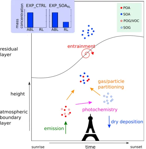
measurements with regional model results and satellite observations. The high-nonfossil fraction of OA that they observed during the summer campaign further points at the transport of regional biogenic SOA into the Greater Paris region and to SOA formation from cooking activities. Finally, Couvidat et al. [2013], using a regional model with surrogate species for hydrophobic and hydrophilic SOA, could not reproduce the diurnal cycle of observed organic carbon over Paris well. Since the local OA formation is minor, other processes may contribute significantly to the OA evolution over Paris. In this study, we focus on local processes and analyze how the interplay of emissions, photochemical production, and vertical mixing affect the budget of both POA and SOA (Figure 1).
For this purpose, we combine the approaches of Dzepina et al. [2009], Hayes et al. [2015], and Janssen et al. [2012, 2013] and conduct (1) a speciation of OA sources, (2) a comparison with observed oxygen to carbon (O:C) ratios, and (3) sensitivity analyses to (i) residual layer OA concentrations, (ii) aging, emission, and deposition assumptions.
Finally, in a series of systematic sensitivity analyses we will show how errors in the representation of ABL growth and of early morning and residual layer SOA concentrations influence the performance of models compared to observations.
In section 2 we describe the observations and the model that we used, in section 3 we discuss the results of the main simulations, and in section 4 the additional sensitivity simulations. Finally, in section 5 the implications for 3-D model studies are discussed.
2. Method
To investigate the governing processes of the OA budget over a suburban site in Paris, we combine the MXL/MESSy one-dimensional model [Janssen and Pozzer, 2015] that simulates the processes that drive the diurnal cycle of OA with a suite of observations. The described model setup applies to the control experiment (EXP_CTRL), unless noted otherwise.
2.1. Observations
The MEGAPOLI campaign provides a comprehensive set of observations including measurements of aerosol concentration and composition, gas phase species, and ABL meteorology. It was conducted during summer 2009 and winter 2010 at various sites in the Greater Paris region. We chose to use data that were collected
Figure 1. Processes controlling the local OA budget over Paris. Processes are indicated by the arrows. Open and closed
circles depict gases and aerosols, respectively. The main experiments as performed in this study (see section 2.3) are indicated in the blue box, where ABL stands for atmospheric boundary layer and RL for residual layer.
during the summer campaign at the suburban SIRTA site (“Site Instrumental de Recherche par Télédétection Atmosphérique”; latitude 48.71∘N, longitude 2.21∘E, 60 m above sea level), located 14 km SW of the Paris City center [Haeffelin et al., 2005]. The SIRTA site provides the most complete data set, including a five-factor PMF solution of the OA (see Table A2 in Appendix A) [Crippa et al., 2013]. This included HOA (hydrocarbon-like OA), COA (cooking OA), SV-OOA (semivolatile oxygenated OA), LV-OOA (low-volatility oxygenated OA), and MOA (marine OA). HOA and COA are from primary sources [Crippa et al., 2013]. They are lumped in this study and compared to modeled POA. SV-OOA represents the fresh SOA and will therefore be compared with modeled SOA characteristics. LV-OOA is likely aged SOA and is probably affected by regional transport. MOA is thought to be partly of marine biological origin [Crippa et al., 2013]. The latter two factors cannot be accounted for in our model, because they have been transported over long distances and are aged on their way.
One day (28 July 2009) is selected for a case study based on (1) the low wind speed, which enables us to minimize the possible effects of advection, (2) clear sky conditions, to minimize the influence of clouds on ABL development and photochemistry, and (3) the availability of data. This day is representative of the MEGAPOLI summer campaign conditions, with observations of OA, gas phase chemistry, and meteorology generally within 1 standard deviation of the campaign average diurnal cycle (Figures S1–S3 in the supporting information). Due to requirements mentioned above, all possible case study days fall within the “Atlantic Polluted” regime [e.g., Freutel et al., 2013] with stagnant conditions and relatively high OA concentrations. However, the comparison of the case study with campaign mean conditions shows that the OA factors that are driven by local processes (SV-OOA and HOA + COA) follow a similar diurnal cycle (Figure S3). Also, most observations from the case study fall within 1 standard deviation of the campaign mean. In contrast, the OA factors mostly affected by long-range transport (LV-OOA and MOA) show a different diurnal pattern for the case study and the campaign mean. Therefore, the case study is representative for the locally influenced OA factors.
In addition to the aerosol mass spectrometer observations, we used measurements of inorganic gas phase species (O3, NOx, HOx) [Michoud et al., 2012], volatile organic compounds [Michoud et al., 2012; Ait-Helal et al.,
2014], and boundary layer meteorology to evaluate our model. 2.2. Model Representation of the Relevant Processes
We used MXL/MESSy (v1.0) [Janssen and Pozzer, 2015] to simulate the processes that drive the diurnal evolu-tion of OA in a single atmospheric column. MXL/MESSy is part of the Modular Earth Submodel System (MESSy), a generalized and flexible interface for the coupling of submodels for Earth system processes [Jöckel et al., 2010]. For this work, we used MESSy version 2.50. In MXL/MESSy, the diurnal dynamics of the boundary layer are represented by the MXL (MiXed Layer) submodel [Janssen and Pozzer, 2015], which accounts for the growth of the well-mixed convective ABL due to entrainment of air from the layer aloft. It accounts for the exchange of scalars and reactive species between the ABL and the layer of air above the ABL. We call this layer the residual layer (RL), because it is likely that in the early morning the ABL is capped by the residual boundary layer that remained when the ABL of the previous day collapsed at the end of the afternoon. Consequently, the physical and chemical characteristics of this ABL are preserved in the RL. When the new ABL starts to grow, air from this RL is entrained first. Only in the afternoon, the ABL will be in contact with the free troposphere, but then entrainment plays a minor role. Mixed-layer theory states that the turbulent convection is strong enough to mix scalars and reactants perfectly throughout the ABL [Vilà-Guerau de Arellano et al., 2015]. Scalars and reactants are therefore characterized by a single value over the whole depth of the ABL.
The gas phase chemistry leading to the formation of condensable organic gases is described by the MIM2 mechanism [Taraborrelli et al., 2009] plus additional reactions for lumped S/IVOCs, aromatics, alkenes, alkanes, and terpenes as described in Tsimpidi et al. [2014].
The ORACLE (v1.0) [Tsimpidi et al., 2014] submodel represents gas/particle partitioning and chemical aging of semivolatile organic compounds (SVOCs) and intermediate volatility organic compounds (IVOCs) that are lumped into logarithmically spaced bins according to their saturation concentration (C∗). The Murphy et al.
[2014] naming convention is used for the organic components involved in aerosol formation, see Table A1 for an overview of the nomenclature. ORACLE separately accounts for SOA species that originate from anthro-pogenic VOCs (aSOA-v) and from biogenic VOCs (bSOA-v). Further, we account for SVOC and IVOC species that originate from fuel combustion. Species with C∗<103μg m−3are considered SVOCs and species with
103<C∗< 106μg m−3are IVOCs. ORACLE considers only homogeneous gas phase aging of S/IVOCs with OH.
Note that species with prefix a and f both originate from anthropogenic sources. The difference between them is that the a (anthropogenic) species are secondary species, formed from VOCs, while the f (fossil fuel) species originate from SVOCs and IVOCs which can be oxidized in the atmosphere and form secondary species [Tsimpidi et al., 2014].
The elemental oxygen to carbon (O:C) ratios for the individual OA species are calculated with the approach of Murphy et al. [2011]. The organic matter to organic carbon ratio (OM/OC) can be expressed as a function of O:C [Murphy et al., 2011, equation (2)] in which H/C (the ratio of moles of hydrogen to moles of carbon) is also a function of O:C [Murphy et al., 2011, equation (3)]. Therefore, we assume an initial O:C for our species and we calculate the initial OM/OC based on equation (2) from Murphy et al. [2011]. The OM/OC after oxidation is the initial OM/OC multiplied by 1.15 for SOA-s/iv and 1.075 for SOA-v, which expresses the increase of mass due to the addition of 2 and 1 oxygens, respectively. This is based on the assumption that carbon is conserved when an organic compound reacts with OH. Then the final OM/OC is used for the calculation of O:C after oxidation again from equation (2) of Murphy et al. [2011]. The O:C ratios that we assumed for the species con-tributing to POA and SOA are shown in Table 1. It also shows the O:C ratios for the parameterizations with nine volatility bins that are discussed in section 4.1. To LV-OOA and MOA, we assigned the values of 0.73 and 0.57, respectively, as observed by Crippa et al. [2013]. The observed mass concentrations of these factors are then used to calculate their contribution to the overall O:C ratio. Oxygenated SOA species that originates from the second or higher generation of oxidation of anthropogenic VOCs (aOSOA-v) are treated as a separate species, because they have different O:C ratios than aSOA-v.
Finally, we use the DDEP submodel [Kerkweg et al., 2006] to calculate dry deposition of gas phase species as a function of resistances that are regulated by atmospheric turbulence and land surface characteristics. In the control case, all SVOC and IVOC species have a Henry’s law constant (H) of 1⋅ 105M atm−1[Tsimpidi et al., 2016].
Table 1. O:C Ratios for the Different Volatility Bins and OA Species in ORACLE, and for the Various
Parameterizations of S/IVOC Aging log(Ca)
Tracer Name Parameterization −2 −1 0 1 2 3 4 5 6 fPOAa ORACLE − 0.17 − 0.10 − 0.06 − 0.00 −
fSOA−svb ORACLE − 0.26 − − − − − − −
fSOA−ivb ORACLE − 0.49 − 0.30 − 0.14 − − −
fPOAa ROB07, GRI09 0.17 0.14 0.12 0.10 0.08 0.04 0.02 0.01 0.00 fSOA−svb ROB07 0.35 0.26 0.21 0.16 − − − − fSOA−ivb ROB07 0.63 0.52 0.42 0.33 0.24 0.16 0.11 0.07 fSOA−svb GRI09 0.80 0.51 0.49 − − − − − fSOA−ivb GRI09 2.17 1.31 1.28 0.67 0.65 0.39 0.37 − bSOA−vb − − 0.40 0.24 0.14 0.10 − − − aSOA−vb − − 0.60 0.40 0.30 0.25 − − − aOSOA−vb − − 0.54 0.44 0.34 − − − − aO:C ratios for fPOA species are based on Donahue et al. [2012].
bO:C ratios for fSOA-sv, fSOA-iv, bSOA-v, and aSOA-v species are based on Murphy et al. [2011].
2.2.1. Model Input
For the emissions of gas and particulate species, we used the emission inventory from Airparif [2010] as in
Fountoukis et al. [2013], with a resolution of 4 × 4 km. The grid cell in which the Sirta site lies was chosen. The
organic carbon (OC) emissions show two peaks (Figure S4), associated with the traffic peaks in the morning and evening. These emissions were partitioned over the volatility bins of the POA from fuel combustion (fPOA) and primary organic gases from fuel combustion (fPOG) species, using the emission factors of Tsimpidi et al. [2014]. The emission database does not include cooking, which can also contribute to POA and S/IVOC emis-sions [Hayes et al., 2015]. For these emisemis-sions, we made the same assumptions as Hayes et al. [2015]: (1) the ratio of the emissions of POA and S/IVOCs from cooking to those from fuel combustion is equal to the ratio between the COA and HOA concentrations (in this case 0.5) and (2) emissions from cooking can be represented by the same volatility distribution as those from fuel combustion. Recently, Fountoukis et al. [2016] included emis-sions from cooking for the greater Paris area as well as in a regional model, using a similar scaling approach as ours. Note that they applied a distinct emission profile from cooking sources with peaks during meal times which was visible in the COA observations at the downtown site, but not at SIRTA.
All other emissions from the database were assigned to the corresponding species in the MIM2 chemical mechanism. Corrections were made for isoprene and NO2, because using the emissions from the database led to an underestimation of the concentrations of these species compared to the observed values and consequently a strong overestimation of radical (HOxand ROx) concentrations (Figure S5).
Since emissions of POA and SOA precursors (and other processes that affect their concentrations) are not spa-tially homogeneous, the diurnal cycle in POA and SOA can be affected by advection of OA and its precursors. To estimate the influence of these effects, we have analyzed the spatial distribution of the emissions along the tracks that the air masses followed before reaching the SIRTA site on the day of the case study. We have calculated 24 h back trajectories for these air masses, arriving at 100 m above ground level and plotted them along with the emissions of OC and SOA precursors from the Airparif [2010] emission inventory. Air masses arrived to the site from the southwest to west on 28 July 2009 (Figure S6). It turned out that for the rele-vant anthropogenic species (OC, ARO1, ARO2, ALK4, and ALK5), emissions were quite homogeneous along the trajectories. Figure S6 shows the summed OC emission and its spatial distribution. For the biogenic VOCs (isoprene and terpenes), emissions from the inventory are more heterogeneous. Besides, they are based on model results for the whole European domain [Fountoukis et al., 2013] and downscaled to the 4 × 4 km grid. Figure S7 shows the summed isoprene emissions for our case study. Nevertheless, we are able to repro-duce the diurnal cycles of these species well (see section 3.2), which gives confidence in the validity of the prescribed emissions.
Initial conditions for OA, gas phase species, and dynamics are based on observations, averaged over the first hour of the simulation to average out fast fluctuations of species concentrations in the nocturnal
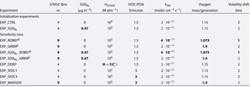
Table 2. Overview of the Main Numerical Experimentsa
S/IVOC Bins SOARL HS/IVOC IVOC/POA kOH Oxygen Volatility shift Experiment nr. (μg m−3) (M atm−1) Emission (molec cm−3s−1) mass/generation bins
Initialisation experiments EXP_CTRL 4 0 105 1.5 2⋅10−11 1.15 2 EXP_SOARL 4 0.47 105 1.5 2⋅10−11 1.15 2 Sensitivity runs EXP_ROB07b 9 0 105 1.5 4⋅10−11 1.075 1 EXP_GRI09b 9 0 105 1.5 2⋅10−11 1.4 2 EXP_SOARL_ROB07b 9 0.47 105 1.5 4⋅10−11 1.075 1 EXP_SOARL_GRI09b 9 0.47 105 1.5 2⋅10−11 1.4 2 EXP_DDEP 4 0 H=f(C∗i) 1.5 2⋅10−11 1.15 2 EXP_IVOC1 4 0 105 1 2⋅10−11 1.15 2 EXP_IVOC3 4 0 105 3 2⋅10−11 1.15 2 EXP_MAXSOA 9 0 105 3 2⋅10−11 1.4 2
aThe bold font shows where the experiment differs from the control experiment (EXP_CTRL). bAlso, MW, emission factors, andΔH
vapdiffer from ORACLE standard.
boundary layer. The initial POA concentration is set to the sum of the observed HOA + COA. The initial SOA concentration is equal to the observed SV-OOA concentration. Early morning SOA is likely from a combina-tion of different sources, but the contribucombina-tion of biogenic, anthropogenic, and/or fuel combuscombina-tion SOA is unknown. We will assume that the sources do not vary much between consecutive days and use the ratio between aSOA-v, bSOA-v, fSOA-sv, and fSOA-iv at the end of a model run in which there was no initial SOA present. This leads to the following distribution: aSOA-v: 39%, bSOA-v: 8%, fSOA-sv: 11%, and fSOA-iv: 42%. In the RL, the concentrations of all OA species are set to zero for the control case (EXP_CTRL) and are subject to sensitivity analysis as described in section 2.3. Mixing ratios of gas phase species in the RL are set to values that gave the best fit with the observations (Table S2). Initial conditions for the MXL dynamics are chosen to give the optimal fit with the observations (Table S1).
2.3. Numerical Experiments
We designed a set of numerical experiments to explore the sensitivities of simulated OA to uncertainties in various processes that determine its diurnal cycle (Table 2). The control experiment (EXP_CTRL), based on the default settings of ORACLE, is used as a basis for further analysis. Our focus is on parameters that are related to the production of SOA and to the influence of vertical mixing due to expansion of the ABL during daytime. In EXP_CTRL, we assume that there is no SOA present in the RL. Then, we perform an experiment in which we explore the sensitivity of simulated SOA to SOA concentrations in the RL: in EXP_SOARL, we optimized the
OA concentration in the RL to obtain the most accurate representation of the OA concentration in the ABL. To this end, we set the concentration of SOA in the RL to 0.47 μg m−3, which is all assigned to the bSOA-v bin
with the lowest saturation concentration (C∗=1 μg m−3). The reason to choose biogenic SOA is that a large
fraction of the SOA in Paris originates from transport of biogenic SOA that is produced from regional sources [Zhang et al., 2013; Beekmann et al., 2015]. However, also multigeneration aging of S/IVOCs or oxidation of relatively long-lived anthropogenic VOCs (e.g., benzene) could lead to the formation of SV-OOA at higher altitudes [e.g., Heald et al., 2011]. However, the validity of the results does not depend on which assumption on the RL SOA composition is made. For aSOA-v and fSOA-sv, RL concentrations of 1.24 and 0.38 μg m−3,
respectively, give the optimal fit with the observations.
Aircraft observations show (Figure S8) [Freney et al., 2014] that on the day of the case study, SV-OOA concen-trations up to 1 μg m−3can be found up to 3 km. However, this vertical profile was observed in the afternoon
at a location 100 km NE from Paris, so it is hard to tell how representative this observation is for the residual layer over the SIRTA site in the morning. Data from flights on other days show similar patterns with above ABL concentrations of SV-OOA between 0 and 1 μg m−3. A residual layer SV-OOA concentration of 0.47 μg m−3
Figure 2. Diurnal evolution of observed and modeled (a) mixed-layer height (h), (b) mixed-layer potential temperature (𝜃), (c) mixed-layer specific humidity (q), and (d) observed wind speed at several heights and wind direction.
Then, we performed additional sensitivity analyses on gas phase aging parameters, VOC emissions, and dry deposition of S/IVOCs that have been performed before in several other studies [Dzepina et al., 2009, 2011;
Hodzic et al., 2013; Hayes et al., 2015; Knote et al., 2015; Tsimpidi et al., 2017]. These experiments are discussed
in section 4.
3. Results
3.1. Meteorology
MXL/MESSy reproduces the observed ABL dynamics well (Figure 2), with root-mean-square errors (RMSE) for boundary layer height (h), potential temperature (𝜃), specific humidity (q), and 10 m wind speed of 120 m, 0.66 K, 0.52 g kg−1, and 0.54 m s−1, respectively. The ABL development can be divided into three periods:
from 05:00 to 07:30 UTC there is a shallow nocturnal boundary layer of about 350 m. From 07:30 onward, the inversion that caps the nocturnal boundary layer is broken up by the convection induced by the surface heat fluxes. Consequently, the ABL grows rapidly (∼260 m h−1) during this morning transition period. From about
13:00 UTC, the ABL growth slows down and the ABL height stabilizes around 2 km. During the period of strong ABL growth, warm and dry air is entrained from the RL above. Consequently, from 08:00 UTC onward𝜃 rises, closely following the ABL growth, and q steeply decreases, after rising first, due to the evaporation flux into the shallow nocturnal boundary layer. Wind speed from observations at various heights by a lidar wind profiler is compared with wind speed from MXL/MESSy. The observed wind speeds are low (≤6 m s−1) but show a height
dependence, caused by friction with the surface. The wind speeds at 100 and 200 m are similar, indicating their convergence to mixed-layer values and, consequently, a surface layer of less than 100 m. Since the direction of the wind is predominantly SW, the observed gas phase and aerosol chemistry are not influenced by advection from the city center of Paris, which is located NE of the SIRTA site.
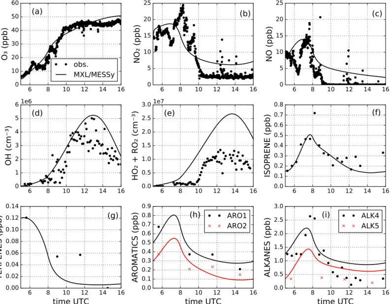
Figure 3. Diurnal evolution of the observed and modeled gas phase species: (a) O3, (b) NO2, (c) NO, (d) OH, (e) HO2+RO2, (f ) isoprene, (g) sum of terpenes, (h) sum of aromatics, and (i) sum of alkanes.
The ABL development at SIRTA is likely representative for that over the greater Paris area, including the city center: the ABL development at the downtown site of Jussieu, located to the northeast of SIRTA (latitude 48.87∘N, longitude 2.33∘E), has a very similar evolution as that at SIRTA for our case study (not shown). Furthermore, Dupont et al. [1999] and Pal et al. [2012] found only minor differences (less than 100 m) in ABL height under convective conditions between the city center and the suburban SIRTA site, even though the sensible heat flux was 20–60% less at the surburban site than in the city center. Moreover, well-mixed temper-ature profiles from radio sondes launched at SIRTA [Dupont et al., 1999] support the validity of the assumption of a well-mixed ABL.
3.2. Gas Phase Chemistry
The main characteristics of the diurnal evolution of most gas phase species are reproduced satisfactorily. The diurnal evolutions of the main oxidants O3and OH are captured well, as shown in Figure 3, with RMSE’s of 3.7 ppb and 1.2⋅ 106molec cm−3, respectively, which ensures the realistic representation of the oxidation of
VOCs and S/IVOCs. Simulated OH is within the combined measurement variability and uncertainty, which is estimated to be 35% [Michoud et al., 2012].
The general characteristics of the diurnal cycles of the VOCs are reproduced satisfactorily (Figure 3). Most VOC concentrations have a peak in the early morning, due to emissions into a shallow ABL, and decline when
the ABL starts growing after 07:30 UTC. Budget calculations show that toward the end of the afternoon, they increase slightly again as a result of continuing emissions while entrainment and chemical destruction slow down. Terpene concentrations form an exception: they decrease throughout the day because their emissions cannot compensate for the chemical breakdown and the dilution due to entrainment. The terpene concen-tration is the sum of the observed𝛼-pinene, 𝛽-pinene, camphene, and limonene concentrations. MXL/MESSy underestimates the terpene concentration in the late morning. If this underestimation is due to a too high reactivity of the lumped terpene species, it would mean an overestimation of the contribution of terpenes to bSOA-v formation, but other processes, like differential emissions for different terpenes species, could play a role as well. The aromatic VOCs are subdivided into two groups, according to their reactivity and SOA yields. The first group, ARO1, includes toluene and benzenes, and the measured species included in the model mea-surement comparison are toluene, benzene, and ethylbenzene. The model evolution of the second group of aromatics (ARO2) is compared with observations of m,p-xylene and o-xylene. MXL/MESSy reproduces the diurnal cycle of ARO1 and ARO2 well, although the simulated peak around 07:00 UTC is not visible in the measurements due to a gap in the data.
Similar to the aromatics, the alkanes are lumped into two groups according to reactivity and SOA yield. The ALK4 group includes the C4–C6alkanes i-butane, n-butane, i-pentane, n-pentane, and hexane and the ALK5
group, the C9–C16alkanes nonane, n-decane, undecane, dodecane, tridecane, tetradecane, pentadecane, and hexadecane. The C12–C16alkanes are IVOCs [Ait-Helal et al., 2014], and since they are explicitly included in the ALK5 group and implicitly in the emission of lumped IVOCs, SOA formation from these species may be double counted. The depletion of ALK4 in the afternoon is not fully reproduced by the model and the mod-eled ALK5 concentration is overestimated during the whole model run. There can be several reasons for this, including missing species in the observations, an overestimation of the ALK5 emissions or underestimation of the lumped reaction rate. To evaluate the possible effect of the latter on the simulated SOA concentration, we ran a simulation in which the reaction rates of ALK4 and ALK5 were increased with the goal to reproduce the afternoon observations. Although this led to increased aSOA-v concentrations by 12%, the overall SOA con-centration decreased by 13%, since the additional OH consumed due to the higher reactivity of the alkanes reduced the oxidation of the bSOA-v and f-SOA-s/iv precursors.
The morning peaks in NO and NO2are not captured exactly by the model, and the afternoon mixing ratios are
overestimated compared to the observations. One important feature of the NOxlevels is that they influence
the reaction channel of the peroxy radicals (RO2) formed from the VOCs, and thereby the SOA yields. However,
we find that even though the NO mixing ratio drops after 09:00 UTC, we are in a high NOxregime throughout
the run, with more than 90% of the isoprene peroxy radicals reacting with NO. However, the observations suggest a shift toward a low-NOxregime after 10 UTC, when NO mixing ratios drop below detection level.
Since SOA yields from aVOCs and bVOCs are higher under low-NOxconditions, the model underestimates the
SOA formation from these precursors after 10 UTC. However, ORACLE does currently not allow for the combi-nation of low- and high-NOxyields in one simulation, so we can not assess how large this underestimation is.
We expect that it does not critically impact our results, since several experiments (EXP_ROB07, EXP_GRI09, and EXP_IVOC3, see section 4) show that SOA formation is not the major factor in explaining model measurement agreement.
For the experiments other than EXP_CTRL, the variations in simulated gas phase species are minor. For instance, the maximum difference between calculated OH between all the experiments is less than 3%. This is in agreement with the findings of Michoud et al. [2012], who found that VOCs and NO2accounted for≥90% of
the OH sinks during the MEGAPOLI summer campaign, and these species do not change significantly between the different experiments.
3.3. Organic Aerosol
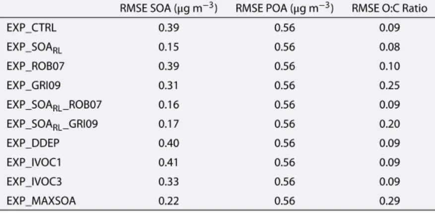
In this section, we describe how the calculated POA and SOA mass concentrations and O:C ratios compare with the observations and how they vary between the numerical experiments. The model measurement discrepancies, as expressed in the average RMSE between 06:00 and 16:00 UTC, are given in Table 3. 3.3.1. Control Case
In the control case (EXP_CTRL), the main characteristics of the diurnal cycle of POA are reproduced well with concentrations that decrease in the morning and stay nearly constant in the afternoon (Figure 4, top). The POA evolution is mainly driven by boundary layer dynamics: when the ABL starts to grow at 07:30 UTC, the early morning POA concentration is diluted by the mixing in of POA-depleted air from the RL and evaporates
Table 3. Model Measurement Discrepancy for All Simulations, Expressed as the RMSE
Averaged From 06:00 to 16:00 UTC
RMSE SOA (μg m−3) RMSE POA (μg m−3) RMSE O:C Ratio
EXP_CTRL 0.39 0.56 0.09 EXP_SOARL 0.15 0.56 0.08 EXP_ROB07 0.39 0.56 0.10 EXP_GRI09 0.31 0.56 0.25 EXP_SOARL_ROB07 0.16 0.56 0.09 EXP_SOARL_GRI09 0.17 0.56 0.20 EXP_DDEP 0.40 0.56 0.09 EXP_IVOC1 0.41 0.56 0.09 EXP_IVOC3 0.33 0.56 0.09 EXP_MAXSOA 0.22 0.56 0.29
Figure 4. (top) Observed HOA+COA and modeled POA from fuel combustion and cooking (fPOA), (middle) observed SV-OOA and modeled SOA from fuel combustion and cooking (fSOA-sv and fSOA-iv), SOA from anthropogenic VOCs (aSOA-v), and SOA from biogenic VOCs (bSOA-v), and (bottom) observed and modeled O:C ratio evolution based on the control experiment (EXP_CTRL, Table 2).
due to the rising temperature. Comparison with a simulation in which a nonvolatile background POA was assumed showed that evaporation led to only 10% lower POA concentrations, indicating that the dilution effect dominates over evaporation. After the period of strong ABL growth (until 13:00 UTC), the concentra-tion of POA remains almost constant. Emission of fPOA compensates little for the diluconcentra-tion and accounts on average for only 23% of the total modeled POA. This behavior is typical for long-lived species with a large background concentration and low production [Janssen et al., 2012]. When cooking emissions are not included, POA concentrations are 8% lower. This shows that cooking emissions are not as important to explain POA concentrations at SIRTA as they are at the downtown site [Fountoukis et al., 2016], because there is less cooking around SIRTA than in the city center.
Also for SV-OOA, dilution plays a role, since it influences the concentrations of gas phase precursors, the dilu-tion of the emissions, and the early morning concentradilu-tion. Figure 4 (middle) shows that for this case, the dilution is strong enough to cause a decrease of simulated SOA between 07:00 and 09:00 UTC, while the observed SV-OOA shows an increase. This is the consequence of the dilution of the early morning SOA and a SOA production from anthropogenic, biogenic, and fuel combustion secondary organic sources (aSOA-v, bSOA-v, and fSOA-sv and fSOA-iv, respectively) that cannot compensate for this dilution.
When we compare the results of EXP_CTRL with those of Zhang et al. [2013] for the same site and day, we see that in their simulation VBS-T2, which is most similar to our simulation, the background OA dominates and that aSOA-v, bSOA-v, fSOA-s/iv, and fPOA together account for less than 50% of the simulated OA. In our simulation, the sum of POA and SOA accounts for 65% of the OA, while the observed LV-OOA and MOA that constitute the background OA in our case, account for the other 35%. This difference can be explained by the fact that we prescribe the early morning concentrations of POA and SOA, which are generally underesti-mated by Zhang et al. [2013]. Further, our definition of background OA differs from that of Zhang et al. [2013]. In contrast with our results, Couvidat et al. [2013] found that much more bSOA-v than aSOA-v is formed. This can partly be explained by the fact that they included SOA from sesquiterpenes, which we did not. Still, when sesquiterpenes are excluded, biogenic SOA dominates over anthropogenic SOA in their simulations. However, the fact that we can satisfactorily reproduce the measured mixing ratios and diurnal evolution of biogenic and anthropogenic VOCs gives confidence in the representation of the SOA formed from anthropogenic VOCs (aVOC). Therefore, it is likely that the different parameterizations for SOA formation that are used in their and in our models led to different effective SOA yields.
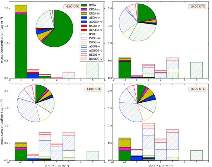
While none of the experiments can be expected to reproduce exactly the observed O:C ratio because of the simplified representation that we use, it is useful to have a look at the general characteristics. For the EXP_CTRL, the simulated O:C ratio is overestimated compared to the observations during the whole model run (RMSE = 0.09), even though the SV-OOA concentration is underestimated. Starting at about 0.30, it increases when the ABL starts growing. This is caused by the increase of the LV-OOA and MOA concentrations (Figure S3), which have a higher oxidation state than the POA which dominates the OA in the early morning. From 11:00 UTC onward, the fresh SOA concentration (with higher O:C ratios than the POA) increases, which leads to a nearly constant O:C ratio of about 0.47, even though the MOA and LV-OOA concentrations decrease. Figure 5 shows the distribution of organic species over the volatility bins for the control case at four different times. At 06:00 UTC, little chemistry or dilution has taken place and therefore the modeled OA mass still mostly reflects the initial conditions that were imposed at the start of the run, dominated by POA (81%). At 13:00 UTC, after the period of strong ABL growth, this percentage has dropped to 52%. From Figure 5 it is also clear that during the day, a large amount of gas phase material is emitted or photochemicaly produced that has the potential for SOA formation upon further oxidation. At 16:00 UTC, it constitutes 80% of the total organic mass, mostly from the oxidation of aVOCs. However, at the low OA concentrations during this campaign (of the order of 100μg m−3), only a very small fraction of the S/IVOCs with C∗>100 μg m−3enters the aerosol
phase. IVOCs are the most important contributors to SOA formation. At 13:00 and 16:00, they contributed 46 and 49%, respectively, to the SOA mass. This is in contrast with the findings of Ait-Helal et al. [2014], who found that on 28 July, SOA formed from VOCs dominated over SOA from IVOCs, based on calculations of observed VOC and IVOC mixing ratios. Explanations for this discrepancy could be the inclusion of unspeciated IVOC emissions from fuel combustion and cooking in our simulations and the multiple generations of oxida-tion that they can follow in the VBS approach. Even when cooking emissions are excluded, the IVOC-derived SOA percentage is still 44 and 45% at 13:00 and 16:00, respectively. Furthermore, the observations of Ait-Helal
Figure 5. Volatility distribution of gas phase and aerosol phase organics at 06:00, 10:00, 13:00, and 16:00 UTC, based on the EXP_CTRL experiment. The solid
colors show the aerosol phase species and the open colors the gas phase organic species. The pie charts represent the mass fraction for each species, summed over all volatility bins.
3.3.2. Entrainment of SOA
In the second experiment (EXP_SOARL), bSOA-v is entrained when the boundary layer starts growing, leading to a rapid increase of SOA during the day, in agreement with SV-OOA observations (Figure 6). The O:C ratio increases less than in EXP_CTRL and is therefore slightly less overestimated (RMSE = 0.08), because the entrained bSOA-v has a relatively low degree of oxidation. POA is diluted as in EXP_CTRL, since the additional SOA does not contribute to the simulated POA, apart from a minor effect on the gas/particle partitioning. The SOA and POA concentrations in this experiment compare most favorably with the observations, as shown by the low RMSE (Table 3).
4. Additional Experiments
In addition to the experiment in which the OA mass concentrations in the RL is varied, we explored some minor sensitivities (Table 2). The entrainment of SOA experiment (i.e., EXP_SOARL) is used as a basis for the
following sensitivity investigations, unless noted otherwise. First, we perform a set of simulations to evaluate how sensitive the modeled fSOA-sv and fSOA-iv are to the gas phase aging parameters and the number of volatility bins, in EXP_ROB07 and EXP_GRI09. Then we evaluate how sensitive our results are to assump-tions on the solubility of S/IVOC species by adapting their Henry’s law constants to recently proposed values [Hodzic et al., 2014; Knote et al., 2015] in EXP_DDEP and we test how the assumed ratio of IVOC to POA emis-sions affects the simulated SOA in EXP_IVOC1 and EXP_IVOC3. Finally, we perform a simulation which aims at producing the maximum amount of SOA, by combining elements from previous experiments (EXP_MAXSOA).
Figure 6. (top) Observed HOA+COA and modeled POA from fuel combustion and cooking (fPOA), (middle) observed SV-OOA and modeled SOA from fuel combustion and cooking (fSOA-sv and fSOA-iv), SOA from anthropogenic VOCs (aSOA-v), and SOA from biogenic VOCs (bSOA-v), and (bottom) observed and modeled O:C ratio evolution, based on the EXP_SOARLexperiment (Table 2) with bSOA-v01(RL)= 0.47μg m−3.
4.1. Sensitivity to Aging Parameters
The formation of SOA from primary semivolatile and intermediate volatility organic compounds (S/IVOCs) is subject to large uncertainties, which are reflected in the different sets of VBS parameters that are commonly used [Dzepina et al., 2009, 2011; Pye and Seinfeld, 2010; Hayes et al., 2015; Tsimpidi et al., 2017]. Therefore, we compare the results from the ORACLE parameterization with those of the parameterizations of Robinson
et al. [2007] (hereafter: ROB07) and Grieshop et al. [2009] (hereafter: GRI09) in EXP_ROB07 and EXP_GRI09,
respectively. The differences between these parameterizations and the standard ORACLE parameterization are shown in Table 2. They differ in the number of bins, the reaction rate of S/IVOCs with OH, the oxygen mass that is added per generation of oxidation, and the number of volatility bins that an S/IVOC shifts per generation of oxidation.
We find that the experiments in which the ROB07 and the GRI09 parameterizations were used, although differing in S/IVOC aging parameters, do not show qualitatively different outcomes than the control case (EXP_CTRL). When there is no OA present in the RL (as in EXP_CTRL), both parameterizations lead to an underestimation of the SOA concentration compared to the observations (Table 3 and Figures S9 and S11). When EXP_SOARL is repeated with the ROB07 and GRI09 parameterizations, we find the following: for
Figure 7. (top) Observed HOA+COA and modeled POA from fuel combustion and cooking (fPOA), (middle) observed SV-OOA and modeled SOA from fuel combustion and cooking (fSOA-sv and fSOA-iv), SOA from anthropogenic VOCs (aSOA-v), and SOA from biogenic VOCs (bSOA-v), and (bottom) observed and modeled O:C ratio evolution, based on the EXP_ROB07_SOARLexperiment (Table 2).
In the former, the SOA and POA mass concentrations are slightly lower and the O:C ratio higher (RMSE= 0.16 μg m−3, 0.56 μg m−3, and 0.10, respectively). Note, however, that in the EXP_SOA
RLthe SOA concentration
in the RL was tuned to obtain the best fit with the observed SOA mass in the ABL, so we cannot objectively decide from these results which parameterization performs better.
For EXP_GRI09_SOARL, SOA mass concentration is captured well (Figure 8, RMSE = 0.17 μg m−3), but the O:C
ratio is strongly overestimated (RMSE = 0.23). The GRI09 parameterization leads to higher O:C ratios than ROB07, due to the more aggressive aging and oxygen addition per oxidation step (Table 2). In previous studies, it was found that GRI09 overestimates OA mass, while simulating the O:C ratio accurately [Dzepina et al., 2011;
Hayes et al., 2015]. Since we prescribe the SOA concentration in the RL here, it is the higher O:C ratio of the
entrained SOA that leads to the overestimation of the O:C in the ABL. Overall, while there are significant discrepancies between the ORACLE, ROB07 and GRI09 parameterizations, we find that the closest model mea-surement match is found when assuming that entrainment of SOA from the RL takes place, irrespective of which parameterization is used.
4.2. Sensitivity to Dry Deposition
To evaluate the effects of assumptions on the dry deposition of S/IVOCs on simulated SOA, we made the Henry’s law constants for S/IVOCs volatility dependent. Instead of a H of 1⋅ 105 M atm−1 for all S/IVOCs
Figure 8. (top) Observed HOA + COA and modeled POA from fuel combustion and cooking (fPOA), (middle) observed
SV-OOA and modeled SOA from fuel combustion and cooking (fSOA-sv and fSOA-iv), SOA from anthropogenic VOCs (aSOA-v), and SOA from biogenic VOCs (bSOA-v), and (bottom) observed and modeled O:C ratio evolution, based on the EXP_GRI09_SOARLexperiment (Table 2).
(as in EXP_CTRL), in EXP_DDEP we set H for biogenic and anthropogenic oxidized VOCs to values in the range between 105and 109M atm−1as derived by Hodzic et al. [2014], and for S/IVOCs, we set H to 1⋅ 1010M atm−1
[Knote et al., 2015]. The latter reflects the highest value for H as applied by Knote et al. [2015], and therefore, we evaluate the maximum effect that dry deposition of S/IVOCs would have.
The enhanced Henry’s law constants for S/IVOCs have only limited influence on the simulated OA concentra-tions (Figure S13). The difference in removal of gas phase organics leads to a reduction of less than 5% of the SOA mass compared to EXP_CTRL, a similar number as found by Hodzic et al. [2013] for Mexico City.
4.3. Sensitivity to IVOC Emissions
To evaluate the sensitivity of simulated SOA to the uncertainty in IVOC emissions, we performed two exper-iments in which the fraction of IVOC to POA emission was set to 1 and 3, which encompasses the range of uncertainty found by ROB07. While IVOCs, with a saturation concentration between 103and 106μg m−3, exist
only in the gas phase under atmospheric conditions, they can be oxidized and form products with a lower volatility that contribute to SOA formation.
We find that the simulated SOA at 16:00 UTC is 0.48 and 0.71 μg m−3, for IVOC/POA emissions of 1 and 3,
could be 31% more SOA formed than in the EXP_CTRL, but this is still a strong underestimation (Table 3 and Figure S15).
4.4. Maximum SOA Production
Finally, we designed an experiment to test whether the diurnal evolution of SV-OOA can be reproduced with-out entraining SOA from the RL. To this end, we combined the elements from previous experiments that led to the highest SOA concentration. This means that we use the GRI09 parameterization for SOA formation, an IVOC to POA emission ratio of 3, a Henry’s law constant of 1⋅ 105M atm−1for all S/IVOCs, and assume cooking
emissions are 50% of fuel combustion emissions. Figure S16 shows that the inclusion of all these sources and assumptions on formation efficiencies do not suffice to reproduce the SV-OOA. Most importantly, in this simulation, as well as in all others that do not include entrainment of SOA-rich air, there is a decrease in simu-lated SOA concentration between 08:00 and 10:00, while the SV-OOA concentration increases. Since the OH concentration is still relatively low at this time, formation of fresh SOA is not fast enough to compensate for the diluting effects of the ABL growth. Moreover, the O:C ratio from this simulation shows the largest overes-timation of all runs (RMSE = 0.29, Table 3). These results further emphasize the important role of entrainment on the diurnal evolution of SV-OOA, in the relatively clean conditions simulated here.
4.5. Fossil Versus Modern Carbon Contribution to OA
Based on an analysis of the14C content, Beekmann et al. [2015] found that the majority of the OA (62 ± 8%)
at the LHVP (Laboratoire Hygiène de la Ville de Paris, latitude 48.83∘N, longitude 2.36∘E) site in the center of Paris, is of modern (nonfossil) origin. It is interesting to see whether our model results are consistent with this high modern carbon contribution, although a direct comparison should be made with caution because of the different locations of model and measurement, in a suburban area and in the city center, respectively. For this purpose, we calculated the modern contribution to OA based on the following experiments and assumptions. First, we assume that all long-range transported OA (LV-OOA and MOA) is of nonfossil origin, which is based on the regional background of the LV-OOA and the biological origin of the MOA [Crippa et al., 2013]. Then, of the locally produced SOA, the biogenic fraction is completely nonfossil. Cooking emissions are also considered nonfossil, and they contribute 1/3 of the total POA and S/IVOC concentrations. There is experimental evidence that cooking also leads to emissions of species (alkanes and aromatics) that contribute to the formation of aSOA-v [e.g., Schauer et al., 1999]. However, with no further information on which fraction of the observed alkanes and aromatics is from cooking sources, we assume that this fraction is negligible.
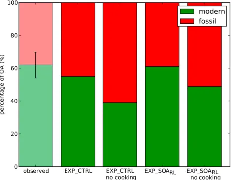
The four experiments with and without cooking emissions and entrainment of biogenic SOA, respectively, show daily average modern carbon contributions ranging between 39 and 61% (Figure 9). The lowest modern carbon contribution is found in EXP_CTRL without cooking emissions, in which the majority (37%) of the modern carbon originates from long-range transport (i.e., the LV-OOA and MOA factors). Including cooking emissions in EXP_CTRL leads to an increase of the modern carbon contribution by 16%. Most of this increase is due to the cooking contribution to fPOA, because its early morning concentration is the highest of all OA factors, and we assume that one third of this initial concentration originates from cooking sources. When we include entrainment of biogenic SOA in EXP_SOA_RL, but no emissions from cooking, the modern carbon con-tribution rises by 10%. Finally, when both cooking emissions and bSOA-v entrainment are included, they lead to a total increase of the modern carbon fraction by 22%, compared to the case in which both are excluded, with similar contributions from cooking and entrainment. In all experiments, the contribution of transport (both vertical and long-range) to modern carbon content dominates over that of local cooking emissions. Nevertheless, a comparison with the14C observations from the city center (Figure 9) suggests that cooking
emissions are still needed to explain the high modern carbon contribution. Since the aerosol composition is very similar at both sites [Beekmann et al., 2015], we do not expect large differences between the14C content
at both sites, although the14C content of the OA at the SIRTA site could be either higher or lower than that
observed in the city center, due to lower traffic and cooking emissions.
5. Implications for the Interpretation of SOA Observations
In the previous sections, we have shown that ABL growth and the subsequent entrainment of SOA from above the ABL are key in understanding the diurnal cycle of SV-OOA over the SIRTA site. This means that these factors have to be taken into account in the interpretation of observations and when comparing 3-D model results with surface-based observations.
Figure 9. Modern versus fossil carbon contribution to OA, based on14C observations from the city center and various
simulations. Results for the EXP_CTRL and EXP_SOARLexperiments are shown, for simulations with and without cooking emissions.
Therefore, in a final analysis, we systematically explore the sensitivity of the model measurement discrep-ancy for SOA to these factors. The fact that we have modeled all relevant components to SOA formation (as opposed to prescribing, e.g., mixing ratios of gas phase reactants or boundary layer height), allows us to perform sensitivity analyses to the coupled system that leads to the SOA evolution during a diurnal cycle. To obtain a complete picture of the effects of vertical mixing, we evaluate this sensitivity for three factors: the ABL height (h), the initial (early morning) SOA concentration in the ABL (SOA0), and the SOA concentration in
the residual layer (SOARL). For simplicity, we assume that all SOA that is initially present in the ABL and RL is of biogenic origin. We studied the impact of ABL dynamics by varying the evaporative fraction (EF) of the sur-face heat flux from 0 to 1, thereby changing the sensible heat flux, the main driver of the ABL development, from 0 (at EF = 1) to 100% (at EF = 0) of the available solar radiation at the land surface [Janssen et al., 2012]. SOA0and SOARLwere varied between 0 and 2 times their optimal value, as established in EXP_SOARL. We also discuss results from the EMAC global model study by Tsimpidi et al. [2014], which used the same submodels for OA formation, gas phase chemistry, and dry deposition as MXL/MESSy.
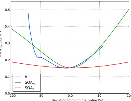
Figure 10 shows the model measurement discrepancy for SOA as a function of SOA0, SOARL, and the diurnally averaged h. The minimum model measurement discrepancy, as expressed in the RMSE of the SOA concen-tration (RMSESOA) between 06:00 and 16:00, is 0.15 μg m−3for the optimal simulation. Note that a slightly
lower RMSE is obtained when h is underestimated by 10%. The RMSESOAis the most sensitive to h and SOARL. An overestimation of h and SOARLled to roughly equal increases of the model measurement error. In EMAC, the SOA concentration in the layer just above the ABL is overestimated by 43 and 123% at 06:00 and 12:00, respectively, with respect to the optimal value of 0.47 μg m−3. This means that the entrainment of SOA would
be overestimated in EMAC if the ABL development is correctly represented. Furthermore, Figure 10 shows that when h is underestimated by more than 50%, the RMSESOAstrongly increases. EMAC underestimates h at
06:00 and 12:00 by 51 and 46%, respectively, compared to the observations. Finally, the sensitivity of RMSESOA
to SOA0is relatively weak, due to the strong dilution of the latter when the ABL grows. In EMAC, however, the
early morning (06:00) SOA concentration in the ABL is underestimated by 245% compared to the observed value, and such an underestimation may still lead to a substantial error in the simulated daytime SOA concen-tration. Obviously, a model with a spatial resolution of hundreds of kilometers cannot be expected to exactly
Figure 10. Sensitivity of the model measurement discrepancy (as expressed in the RMSE for SOA concentrations) to
boundary layer height (h), early morning SOA concentration in the ABL (SOA0), and SOA concentration in the RL (SOARL). Thexaxis shows the deviations of these parameters, relative to their value in the experiment that yielded the best model measurement fit (EXP_SOARL).
reproduce the observed diurnal cycle at a single point in space. However, our results indicate that this is something that has to be kept in mind when comparing the outcomes of such models with local observations in the ABL.
6. Conclusions
We studied the diurnal evolution of the locally influenced organic aerosol factors over a suburban site near Paris, by combining the MXL/MESSy column model with observations. We find that MXL/MESSy reproduces ABL dynamics and gas phase chemistry satisfactorily for this suburban site. Further, we find opposing effects of ABL dynamics on POA and SOA concentrations: while the POA mass concentration is mainly driven by dilution due to ABL growth during daytime, the SOA evolution can only be explained when mixing in of SOA-rich air from the residual layer is invoked. The latter finding is corroborated by vertical profile observations of SV-OOA, and it is independent of which assumptions on S/IVOC emissions or aging parameters are applied. Further, the strong increase of the SV-OOA concentration coincides with the growth of the ABL. Therefore, we con-clude that mixing in of SOA from the RL is essential to explain observed ground level SV-OOA concentrations in Paris, under the relatively clean conditions found during the MEGAPOLI campaign. In contrast, the local pro-duction of POA and SOA is low due to low emissions of POA, S/IVOCs, and biogenic and anthropogenic VOCs. This effect is enhanced by the strong boundary layer development during daytime, which leads to strong dilu-tion of the emissions and the formed aerosol. Almost half of the locally produced SOA is derived from IVOCs, and anthropogenic VOCs form the second most important SOA precursor.
POA and S/IVOC from cooking emissions and entrainment of biogenic SOA contribute equally to the simulated modern carbon content of the OA. However, the combined contribution of vertical and long-range transport dominates as the major modern carbon source to OA over local cooking emissions at the SIRTA site. The impact of vertical mixing on near-surface SOA concentrations should be taken into account when com-paring results from regional and global models to local observations in the ABL: the SOA concentration in the ABL is equally sensitive to the dynamics of the ABL as to the SOA concentration aloft. Finally, to support the adequate interpretation of SOA measurements, in addition to observations of the ABL height, early morning profiles of OA concentrations in the residual layer are crucial.
Table A1. List of ORACLE Species Used in This Paper
Source Root Name Description Modifiers
a Mass from anthropogenic sources (i.e., aSOA) b Mass from biogenic sources (i.e., bSOA) f Mass from fossil fuel combustion (i.e., fPOA) Base terms
POA Primary organic aerosol. This is emitted in the particle phase and has not undergone chemical reaction
POG Primary organic gas that has not undergone chemical reaction SOA Secondary organic aerosol formed from the
oxidation of gas phase organic species
OSOA Oxygenated secondary organic aerosol formed from the second or higher generation of oxidation of gas phase organic species
SOG Secondary organic gas. The gas phase mass produced by at least one chemical reaction in the atmosphere
OSOG Oxygenated secondary organic gas. The gas phase mass produced by at least two chemical reactions in the atmosphere
Initial volatility Suffix
-sv Product of the oxidation of SVOCs -iv Product of the oxidation of IVOCs -v Product of the oxidation of VOCs
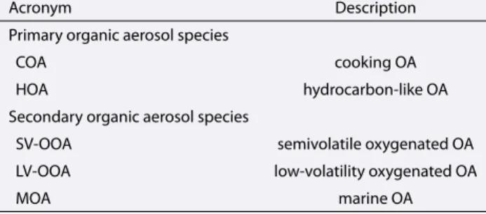
Table A2. List of Observed Organic Aerosol Species Used in This Paper
Acronym Description Primary organic aerosol species
COA cooking OA
HOA hydrocarbon-like OA Secondary organic aerosol species
SV-OOA semivolatile oxygenated OA LV-OOA low-volatility oxygenated OA
MOA marine OA
Appendix A: List of Acronyms
Tables A1 and A2 show lists of ORACLE and observed organic aerosol species used in this paper, respectively.
References
Airparif, (2010), Ile-de-France gridded emission inventory 2005 (version 2008), Tech. Rep. [Available at http://www.airparif.asso.fr.] Ait-Helal, W., et al. (2014), Volatile and intermediate volatility organic compounds in suburban Paris: Variability, origin and importance for
SOA formation, Atmos. Chem. Phys., 14(19), 10,439–10,464, doi:10.5194/acp-14-10439-2014.
Beekmann, M., et al. (2015), In situ, satellite measurement and model evidence on the dominant regional contribution to fine particulate matter levels in the Paris megacity, Atmos. Chem. Phys., 15(16), 9577–9591, doi:10.5194/acp-15-9577-2015.
Blanchard, C., G. Hidy, S. Tanenbaum, and E. Edgerton (2011), NMOC, ozone, and organic aerosol in the southeastern United States, 1999–2007: 3. Origins of organic aerosol in Atlanta, Georgia, and surrounding areas, Atmos. Environ., 45(6), 1291–1302, doi:10.1016/j.atmosenv.2010.12.004.
Couvidat, F., Y. Kim, K. Sartelet, C. Seigneur, N. Marchand, and J. Sciare (2013), Modeling secondary organic aerosol in an urban area: Application to Paris, France, Atmos. Chem. Phys., 13(2), 983–996, doi:10.5194/acp-13-983-2013.
Crippa, M., et al. (2013), Identification of marine and continental aerosol sources in Paris using high resolution aerosol mass spectrometry, J. Geophys. Res. Atmos., 118, 1950–1963, doi:10.1002/jgrd.50151.
Donahue, N. M., J. H. Kroll, S. N. Pandis, and A. L. Robinson (2012), A two-dimensional volatility basis set—Part 2: Diagnostics of organic-aerosol evolution, Atmos. Chem. Phys., 12(2), 615–634, doi:10.5194/acp-12-615-2012.
Dupont, E., L. Menut, B. Carissimo, J. Pelon, and P. Flamant (1999), Comparison between the atmospheric boundary layer in Paris and its rural suburbs during the ECLAP experiment, Atmos. Environ., 33(6), 979–994, doi:10.1016/S1352-2310(98)00216-7.
Acknowledgments
The authors thank Christos Fountoukis for sharing the high-resolution emission inventory, Sacha Kukui for the radical data, and Evelyn Freney for the aircraft data. We thank Johannes Schneider, Friederike Freutel, and Frank Drewnick for helpful discussions. A.P. Tsimpidi acknowledges support from a DFG individual grant program (project reference TS 335/2-1), and V.A. Karydis acknowledges support from a FP7 Marie Curie Career Integration grant (project reference 618349). The measurement data are available from the cited references and the model data are available at doi:10.6084/m9.figshare.5031137.