HAL Id: hal-01335919
https://hal.archives-ouvertes.fr/hal-01335919
Submitted on 22 Jun 2016
HAL is a multi-disciplinary open access
archive for the deposit and dissemination of
sci-entific research documents, whether they are
pub-lished or not. The documents may come from
teaching and research institutions in France or
abroad, or from public or private research centers.
L’archive ouverte pluridisciplinaire HAL, est
destinée au dépôt et à la diffusion de documents
scientifiques de niveau recherche, publiés ou non,
émanant des établissements d’enseignement et de
recherche français ou étrangers, des laboratoires
publics ou privés.
On the diameter of cut polytopes
José Neto
To cite this version:
José Neto. On the diameter of cut polytopes. [Research Report] Dépt. Réseaux et Service
Multi-média Mobiles (Institut Mines-Télécom-Télécom SudParis); Services répartis, Architectures,
MOdéli-sation, Validation, Administration des Réseaux (Institut Mines-Télécom-Télécom SudParis-CNRS).
2013, pp.20. �hal-01335919�
(will be inserted by the editor)
On the diameter of cut polytopes
Jos´e Neto
Received: date / Accepted: date
Abstract Given an undirected graph G with node set V , the cut polytope is defined as the convex hull of the incidence vectors of all the cuts in G. And for a given integer k ∈ {1, 2, . . . , ⌊|V |2 ⌋}, the uniform cut polytope CU T=k(G)
is defined as the convex hull of the cuts which correspond to a bipartition of the node set into sets with cardinalities k and |V | − k.
In this paper, we study the diameter of these two families of polytopes. With respect to the cut polytope, we show a linear upper bound on its di-ameter (improving on one stemming from the reference: [F. Barahona and A.R. Mahjoub: On the cut polytope, Mathematical Programming 36, 157–173 (1986)]), give its value for trees and complete bipartite graphs. Then concern-ing uniform cut polytopes, we establish bounds on their diameter for different graph families, we provide some connections with other partition polytopes in the literature, and introduce sufficient and necessary conditions for adjacency on their 1-skeleton.
Keywords (uniform) cut polytope · diameter · graph partitioning Mathematics Subject Classification (2000) 05C12 · 90C05 · 90C57
1 Introduction
Given a nonempty polytope P , the 1-skeleton of P is defined as the set of vertices and edges of P . Given two vertices v1, v2 of P , let d(v1, v2) denote
the length (w.r.t. the number of edges) of a shortest path in the graph cor-responding to the 1-skeleton of P between the nodes representing v1 and
v2. The diameter of P , which is denoted by diameter(P ) is the maximum
Jos´e Neto
Institut Mines-T´el´ecom, T´el´ecom SudParis, CNRS Samovar UMR 5157, 9 Rue Charles Fourier, 91011 Evry Cedex, France
length of a shortest path between any two vertices of P , i.e. max{d(v1, v2) :
v1, v2 are vertices of P }.
The notion of diameter of a polyhedron presents, among others, some con-nections with linear programming and linear optimization methods that are based on the fact that there exists an optimal solution that is a vertex of the feasible region whenever the latter is nonemtpy and bounded. For example, consider the simplex algorithm applied to a linear program: starting from a particular vertex v0 of the feasible region F (a polyhedron), this method
con-sists in iteratively moving from a vertex (the current basic feasible solution) of F to a neighbor (with better or equal objective value), until an optimal vertex solution v∗ is found. Given a nonempty polytope P , let V (P ) denote the set
of vertices of P and I(P ) denote the set of all the instances of linear pro-gramming problems having P as feasible region. Given an instance I ∈ I(P ) and v0∈ V (P ), let s(I, v0) denote the minimum number of iterations the
sim-plex method may apply before reaching an optimal solution, starting with the vertex s0. Then the diameter provides a lower bound on the quantity:
max
(I,v0):I∈I(P ),v0∈V (P )
{s(I, v0)}
that is, on the number of iterations the procedure applies at least, in a ’worst-case’ (i.e. when the diameter coincides with the distance on the 1-skeleton of P between the starting point v0 and the optimal solution v∗).
For further information on polytopes and related notions, the reader may consult, e.g., the textbooks by Gr¨unbaum [6] and Ziegler [11]. In the present paper we study the diameter of cut polytopes. To be more precise, the poly-topes we consider correspond to the convex hull of the incidence vectors of all the cuts in some given graph or to the convex hull of the incidence vectors of the cuts that satisfy an additional constraint with respect to the cardinali-ties of their shores. Our objective is to develop new insights and improve our knowledge on the polyhedral structure of these notorious and related poly-topes (for further information on properties and applications of these families of polytopes the reader may consult, e.g., [4]). For, in the rest of this section, we introduce some notation and preliminaries.
Notation and preliminaries
Let G stand for an undirected graph with node set V and edge set E. Given a node set S ⊆ V , let δG(S) (or δ(S) when G is clear from the context) stand
for the cut that is defined by S, i.e., the set of edges in E with exactly one endpoint in S: δ(S) = {e ∈ E : |e ∩ S| = 1}. The node sets S and V \ S are called the shores of the cut δ(S).
Given a set F of edges in G, its incidence vector χF ∈ R|E| is defined by
χF
e = 1 if e ∈ F and 0 otherwise. Given a node v ∈ V , N (v) denotes the set of
nodes in V \ {v} that are adjacent to v in the graph G, and deg(v) stands for the degree of this node, i.e. deg(v) = |N (v)|. The dimension of a polyhedron
P is the maximum number of affinely independent points in P minus 1. It is denoted by dim(P ).
Given S ⊆ V , G[S] denotes the subgraph of G that is induced by the node set S.
The cut polytope CU T (G) is defined as the convex hull of the incidence vectors of all the cuts in the graph G, i.e. CU T (G) = conv{χδG(S): S ⊆ V }.
Given some integer k satisfying k ≤ ⌊n
2⌋, CU T=k(G) = conv{χδG(S): S ⊆
V and |S| = k} denotes the convex hull of the incidence vectors of the cuts in G having one shore with size k. Polytopes of the latter form are called uniform cut polytopes. In the particular case when the graph G is complete, we shall simply write: CU Tn
=k.
A d-dimensional polytope P with f facets is said to satisfy the Hirsch property if its diameter verifies the inequality: diameter(P ) ≤ f − d.
To the author’s knowledge, the first study of the 1-skeleton of the cut poly-tope appears in the paper by Barahona and Mahjoub [1]. There, the authors namely provide the following characterization of the adjacency of incidence vectors of cuts on the cut polytope (Theorem 4.1 in [1]).
Theorem 1 Let G = (V, E) be a connected graph. Let xI, xJ be extreme
points of CU T (G); let I, J be the corresponding cuts. Let F = E \ (I∆J). Then xI and xJ are adjacent in CU T (G) iff H
I∆J = (V, F ) has two connected
components.
In the same reference [1] the authors also establish that the Hirsch property holds for CU T (G). In fact, Naddef [10] proved later that this property holds for all (0, 1)-polytopes, and thus also for CU T (G) and the uniform cut polytopes. What also follows from Theorem 1 and its proof is that CU T (G) is a so-called combinatorial polyhedron [8,9], a family of polyhedra for which Matsui and Tamura also established further different properties related to the Hirsch property [8].
The present paper is organized as follows. In Section 2, we study the di-ameter of the cut polytope depending on the graph properties, give its exact value for some cases and provide upper bounds on some other classes. In Sec-tion 3 we report investigaSec-tions on the diameter of uniform cut polytopes: after we discuss some particular cases (Subsection 3.1), we provide (Subsection 3.2) sufficient and necessary conditions for the incidence vectors of two cuts to be adjacent on these polytopes.
2 On the diameter of the cut polytope
For the particular case of complete graphs Barahona and Mahjoub [1] showed that the cut polytope has diameter 1: this is a direct consequence of Theorem 1. For general graphs they provided the following upper bound on the diameter that is given by the next theorem (Theorem 4.3 in [1]). Before we formulate it we give some additional notation. Let G be a connected graph and C be a cut
in G. Let T (C) denote the graph obtained from G by contracting edges not in C and replacing multiple edges by single edges. Let m(C) be the number of edges of T (C). Given two cuts I, J of G, let d(I, J) stand for the distance in the 1-skeleton of CU T (G) between the vertices corresponding to the incidence vectors of I and J.
Theorem 2 If I and J are two cuts in G, then d(I, J) ≤ m(I∆J).
We now give a generally better bound on the distance between the incidence vectors of two cuts in the 1-skeleton of CU T (G). Given a subset of edges I of the graph G, let HI denote the graph obtained from G by removing all
the edges in I. Given a graph G, let κ(G) denote the number of connected components in G.
Proposition 1 If I and J are two cuts in a connected graph G, then d(I, J) ≤ κ(HI∆J) − 1.
Proof First notice that the proposition holds for the two basic cases when HI∆J has one or two components. The case when κ(HI∆J) = 1 corresponds
to I = J, and so d(I, I) = 0 = κ(HI∆J) − 1 = κ(G) − 1. By Theorem 1 we
have d(I, J) = 1 if and only if κ(HI∆J) = 2.
So assume now κ(HI∆J) ≥ 3. Let P = δ(S), ∅ 6= S ( V denote a minimal
(w.r.t. inclusion) proper cut in G which is contained in I∆J. Define L := I∆P . Notice that since P is minimal it follows from Theorem 1 that the cuts I and L have their respective incidence vectors adjacent on the cut polytope CU T (G). Also notice that L is a cut which differs from I only in the set δ(S). More precisely we have L = (I \ δ(S)) ∪ (J ∩ δ(S)). And as the graph G is assumed to be connected we have (I∆J) ∩ δ(S) 6= ∅. This implies that the graph HL∆J
(which differs from HI∆J only in the set of edges δ(S)) will contain at least
one edge in δ(S), and thus κ(HL∆J) ≤ κ(HI∆J) − 1.
We may then iterate this process (i.e. look for a minimal cut P′ in G that
is contained in L∆J, then define L′ = L∆P′ . . . ) until the graph H which
is built at the current iteration (i.e. as HI∆J above) has only two connected
components (which, by Theorem 1, corresponds to the case when a cut, whose incidence vector is adjacent to the one of J on the cut polytope, has been reached).
As the number of connected components of the graph H decreases by at least one at each iteration and each operation of the form I∆P (as described above) corresponds to moving from one vertex to an adjacent one on the cut polytope, it follows that d(I, J) ≤ κ(HI∆J) − 1.
Remark. To be more accurate, one can give the following upper bound on d(I, J). The underlying idea is to use a minimal cut that is contained in I∆J and induces the maximum reduction in the number of connected components in the auxiliary graph H that will be used in the next iteration. We have: d(I, J) ≤ κ(HI∆J) − ηI,J with
ηI,J = maxC=I,J{cn(S, C) : δ(S) minimal cut of G contained in I∆J}. Given
different connected components (Ci)ri=1 in HI∆J, none of which is contained
in S and such that for each component Cj, j ∈ {1, . . . , r} there is an edge in
C having one endnode in S and the other in Cj.
For any connected graph G, Proposition 1 provides the upper bound n − 1 on the diameter of the cut polytope CU T (G). This bound can also be shown to hold and improved for disconnected graphs. But before we give an improved bound, we shall first mention some results with respect to the diameter and the adjacency relation between vertices of cartesian products of polyhedra. The proofs are simple and given here for completeness and since the author is not currently aware of a reference in the literature stating them explicitly.
Given a set of q ∈ N, q ≥ 2, polyhedra (Pi)qi=1 with Pi ⊆ Rni, ni ∈ N,
for all i ∈ {1, 2, . . . , q}, their cartesian product is the set P = ×i=1,...,qPi =
{(x1, x2, . . . , xq) ∈ ×i=1,...,qRni: xi∈ Pi, i = 1, . . . , q}.
Proposition 2 The vector (x1, x2, . . . , xq) ∈ P (= ×i=1,...,qPi) is an extreme
point of P if and only if xi is an extreme point of Pi, for all i ∈ {1, 2, . . . , q}.
Proof [⇒] Assume the vector x = (x1, x2, . . . , xq) is an extreme point of the
polyhedron P and that some vector xk, k ∈ {1, 2, . . . , q}, is not an extreme
point of Pk. Then, there exist different vectors yk1, yk2∈ Pk, α ∈]0, 1[ such that
xk = αy1k+ (1 − α)yk2. Let zi = (x1, . . . , xk−1, yki, xk+1, . . . , xq), for i = 1, 2.
Since both vectors z1, z2, belong to the polyhedron P and x = αz1+ (1 − α)z2,
we get a contradiction with x being an extreme point of P .
[⇐] Assuming that all the vectors xifor i = 1, . . . , q are extreme points of the
polyhedra (Pi)qi=1 implies that the vector x = (x1, x2, . . . , xn) belongs to P
and cannot be expressed as a convex combination of other points in P . Thus, x is an extreme point of P .
Proposition 3 Let x = (x1, x2, . . . , xq) and y = (y1, y2, . . . , yq) denote two
different extreme points of the polyhedron P . Then, x and y are adjacent on the 1-skeleton of P if and only if
i) |{i ∈ {1, 2, . . . , q} : xi6= yi}| = 1, and
ii) xk and yk are adjacent extreme points on the 1-skeleton of Pk, with k ∈
{1, 2, . . . , q} and such that xk6= yk.
Proof [⇒] Necessity of i). Assume that the vectors x and y are such that xr 6= yrand xs6= ys for at least two different indexes r, s ∈ {1, 2, . . . , q}. Let
w = (x1, . . . , xr−1, yr, xr+1, . . . , xq), and z = (y1, . . . , yr−1, xr, yr+1, . . . , yq).
Since w and z both differ from the vectors x, y and are two different points of P such that x + y = w + z, we get a contradiction with x, y being adjacent extreme points of P .
Necessity of ii). We make use of the property that two extreme points x1, x2,
of a polyhedron Q ⊆ Rn are adjacent if and only if there exists some vector
c ∈ Rn such that x1 and x2 are the only two extreme points of Q which
maximize ctx over x ∈ Q.
Let c = (c1, c2, . . . , cq) ∈ ×i=1,...,qRni be a vector such that the optimum of
point of P . Then, necessarily the vector ck ∈ Rnk is such that the linear
program maxx∈Pkc
tx is attained by x
k and yk but no other extreme point of
Pk.
[⇐] Let x = (x1, x2, . . . , xq) and y = (y1, y2, . . . , yq) denote two
differ-ent extreme points of P such that properties i) and ii) hold. For each j ∈ {1, 2, . . . , q} \ {k}, let cj ∈ Rnj denote a vector such that xj is the only
ex-treme point of Pj which is optimal for the linear program maxx∈Pjc
t jx. And
let ck ∈ Rnk be such that the linear program maxx∈Pkc
tx is attained by
xk and yk but no other extreme point of Pk. Considering now the vector
c = (c1, c2. . . , cq) it is obvious that x and y are the only two extreme points
of P attaining the optimum of the linear program maxx∈Pctx.
Proposition 4 The following equation holds
diameter(P ) =
q
X
i=1
diameter(Pi).
Proof Let the sequence of extreme points of the polyhedron P : (xk)L
k=0, L ∈ N,
denote a shortest path τ in the 1-skeleton of P (w.r.t. the number of edges) joining two of his extreme points: x = (x1, x2, . . . , xq) and y = (y1, y2, . . . , yq).
Let τ = (x0 = x, x1, . . . , xL = y), with xj = (xj 1, x
j
2, . . . , xjq), j = 0, . . . , L.
From Proposition 3 and removing redundancies, the sequence (xk
i)Lk=0 with
i ∈ {1, 2, . . . , q}, corresponds to a shortest path τi in the 1-skeleton of Pi
joining xi and yi, and the length l(τ ) (i.e. the number of edges) of the path
τ corresponds to the sum of these paths τi, i = 1, . . . , q: l(τ ) =Pqi=1l(τi). It
follows that diameter(P ) ≤Pq
i=1diameter(Pi).
Now, for each i ∈ {1, 2, . . . , q}, let (xi, yi) denote a pair of extreme points
of the polyhedron Pi such that their distance in the 1-skeleton of Pi equals
diameter(Pi). Then, considering the length of a shortest path τ in the
1-skeleton of P joining its extreme points x = (x1, x2, . . . , xq) and y = (y1, y2, . . . ,
yq), from Proposition 3, we deduce diameter(P ) ≥ l(τ ) ≥Pq
i=1diameter(Pi).
A corollary of Proposition 4 is the following result relating the diameter of CU T (G) to that of the cut polytopes corresponding to the connected compo-nents of the graph G.
Corollary 1 For a graph G = (V, E) with connected components correspond-ing to the subgraphs (Gi = (Vi, Ei))ri=1, r ≥ 2, the following equation holds :
diameter(CU T (G)) =Pr
i=1diameter(CU T (Gi)).
Proof The result follows from Proposition 4 and the relation CU T (G) = ×r
i=1CU T (Gi).
Corollary 2 For any graph G = (V, E) we have diameter(CU T (G)) ≤ |V | − κ(G).
Proof Applying Corollary 1 and using the upper bound |Vi|−1 on the diameter
of CU T (Gi) for each connected subgraph Gi = (Vi, Ei) of G (which follows
Remark. Notice that for the case of trees, for example if we consider a tree with n nodes, then the cut polytope has dimension n − 1 and 2(n − 1) facets (each one corresponds to a trivial inequality), so that the diameter (by Proposition 6) coincides here with the number of facets minus the dimension of the polytope. So, in some sense, this class of graphs is tight for the Hirsch property.
The upper bounds given by Theorem 2 and Corollary 2 on the diameter of the cut polytope are both tight for trees. However, for general graphs, both may strongly differ. For, we mention hereafter a case where the bound from Theorem 2 may be quadratic in the number of vertices of the graph whereas the one from Corollary 2 is linear. Consider the case of a complete bipartite graph Kk1,k2 with node bipartition (V1, V2) with |Vi| = ki for i = 1, 2. The upper bound on the diameter of CU T (Kk1,k2) provided by Theorem 2 is k1k2 whereas that from Corollary 2 is n − 1 = k1+ k2− 1.
Note that the value k1k2 from Theorem 2 corresponds to C = I∆J with
I = ∅ and J = δ(V1) (or vice-versa). Assume without loss of generality k1≤ k2.
Proceeding as in the proof of Proposition 1 we can show d(δ(∅), δ(V1)) ≤ k1.
Although better, we will see next that the bound from Corollary 2 is not tight in general, e.g., for the case of complete bipartite graphs by showing that the value of the diameter of the cut polytope for a family of such graphs is 2 (see Proposition 7).
Proposition 5 Let G2= (V, E′) be a connected subgraph of G1= (V, E) and
let S1, S2 denote two subsets of the node set V . Then if the incidence vectors
of the cuts δ(S1) and δ(S2) are adjacent on CU T (G2), they are also adjacent
on CU T (G1).
Proof Assuming δG2(S1) and δG2(S2) are adjacent on CU T (G2), then from Theorem 1, the graph H2= H
δG2(S1)∆δG2(S2), has two connected components. Since E′ ⊆ E, each connected component of H2 is contained in one of H1 =
HδG1(S1)∆δG1(S2) (defined similarly as H
2 with respect to the graph G1). So
κ(H1) ≤ 2 and since δ
G1(S1) 6= δ
G1(S2), necessarily κ(H1) ≥ 2. So κ(H1) = 2 and by Theorem 1, the incidence vectors of the cuts δG1(S1) and δ
G1(S2) are adjacent on CU T (G1).
Corollary 3 Let G2= (V, E′) be a connected subgraph of G1= (V, E). Then
diameter(CU T (G2)) ≥ diameter(CU T (G1)).
Proof Let vi
S denote the vertex in the 1-skeleton of Gi corresponding to the
cut δGi(S), for i = 1, 2, S ⊆ V . Let S1, S2 ⊆ V , S1 6= S2 and consider a shortest path (w.r.t. the number of edges) (v0= vS21, v1, . . . , vl= v
2 S2) joining v2 S1 and v 2 S2 in the 1-skeleton of CU T (G
2). From Proposition 5 the sequence
of cuts corresponding to this path also corresponds to a path in the 1-skeleton of CU T (G1) (joining v1
S1 and v
1 S2).
From Corollary 3, it follows that among the connected graphs, the trees constitute a class with largest diameter with respect to the cut polytope. Since
the cut polytope of a tree with n+1 nodes corresponds to the hypercube [0, 1]n,
we deduce the following proposition.
Proposition 6 If G = (V, E) is a tree, then diameter(CU T (G)) = |V | − 1. Proposition 7 For any two integers k1, k2 ≥ 2, diameter(CU T (Kk1,k2)) = 2.
Proof Let (V1, V2) denote the node bipartition associated with the graph Kk1,k2. (So we have |Vi| = ki for i = 1, 2). We start defining four types of cuts in
G = Kk1,k2:
– Type 0: δ(∅) = δ(V ) = ∅. – Type 1: δ(V1) = δ(V2).
– Type 2: δ(W ) = δ(V \ W ) with W such that Vi\ W 6= ∅ and W ∩ Vi 6= ∅
for i = 1, 2.
– Type 3: δ(W ) = δ(V \ W ) with W 6= ∅ such that either W ( V1or W ( V2.
From Theorem 1, it follows that each cut of type 0 or 1 is adjacent to all the cuts of type 2. This implies that the distance in the 1-skeleton of CU T (Kk1,k2) between two cuts having their types in the set {0, 1, 2} is at most 2.
The following three claims imply that the distance between a cut of type 3 and another one of type 0, 1 or 3 is at most 2.
Claim 1. If ∅ 6= Wi(V
ifor i = 1, 2, then the incidence vectors of the cuts
δ(Wi) for i = 1, 2 are adjacent on CU T (G).
Proof of Claim 1. Let δi= δ(Wi) for i = 1, 2. Then the claim follows by
The-orem 1, observing that the graph Hδ1∆δ2 has two connected components: they correspond to the node sets W1∪ W2 and its complement in G. ⋄
Note that in the following claim the node sets W1 or W2 may correspond
to the empty set ∅. The case W1, W2⊆ V
2 is symmetric.
Claim 2. Assume W1, W2⊆ V
1. Then the incidence vector of the cut δ(W1∪
W2∪ {z}) with z ∈ V
2 is adjacent on CU T (G) to the incidence vectors of the
cuts δ(Wi) for i = 1, 2.
Proof of Claim 2. Let W′ := W1∪ W2∪ {z}. The claim follows by Theorem
1, observing that the graphs Hδi∆δ′ with δi= δ(W
i) and δ′= δ(W′) have two
connected components: they correspond to the node sets Wi∪ (V
1\ W′) ∪ (V2\
{z}) and its complement in G, for i = 1, 2. ⋄
It remains to consider the distance between two cuts, one of which is of type 2 and the other of type 3. So assume δ(W1) and δ(W2) are two cuts of
type 2 and 3 respectively, with W1 ⊂ V and W2 ( V
1 (the case W2 ( V2
is symmetric). Consider now a set U which consists of four nodes in G: U = {v1, v2, z1, z2} and satisfying the following requirements:
– Properties verified by the nodes v1, v2. We distinguish between two cases.
First, if (W1∩ V
1) \ W26= ∅ and W2\ W16= ∅, then v1∈ (W1∩ V1) \ W2
and v2∈ W2\ W1. Otherwise (i.e. W2⊆ (W1∩ V1) or (W1∩ V1) ⊆ W2),
– Properties verified by the nodes z1, z2: z1∈ W1∩ V2 and z2∈ V2\ W1.
Claim 3. The incidence vector of a cut δ(U ) in G satisfying the two properties mentioned above is adjacent to the incidence vectors of the cuts δ(W1) and
δ(W2) on CU T (G).
Proof of Claim 3. The claim follows from Proposition 1. For the two cases mentioned above concerning the properties verified by the nodes v1 and v2
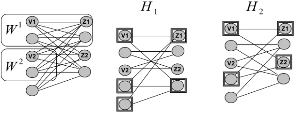
in U , we mention explicitly the node set corresponding to one of the two connected component arising in the graphs Hδ(Wi)∆δ(U) for i = 1, 2. To ease the exposition, an illustration is provided for each case by the Figures 1 and 2.
Fig. 1 Illustration for the proof of Proposition 7 on the graph K5,4: case (W1∩V1)\W26= ∅
and W2\ (W1∩ V
1) 6= ∅. The first graph gives the sets W1and W2. The second and third
graphs correspond to Hi= Hδ(Wi)∆δ(U )for i = 1, 2, respectively, showing by Proposition 1
that the incidence vectors of the cuts δ(Wi) and δ(U ) are adjacent on CU T (G). The set of
nodes that are squared in H1and H2 correspond to one of the two connected components
in those graphs.
– Case (W1∩ V
1) \ W2 6= ∅ and W2\ W1 6= ∅. One of the two connected
components of the graph Hδ(Wi)∆δ(U) corresponds to the node set {v1} ∪ (V1\ (W1∪ {v2})) ∪ {z1} ∪ (V2\ (W1∪ {z2})) for i = 1 and to the node
set {v1, z1, z2} ∪ W2\ {v2} for i = 2.
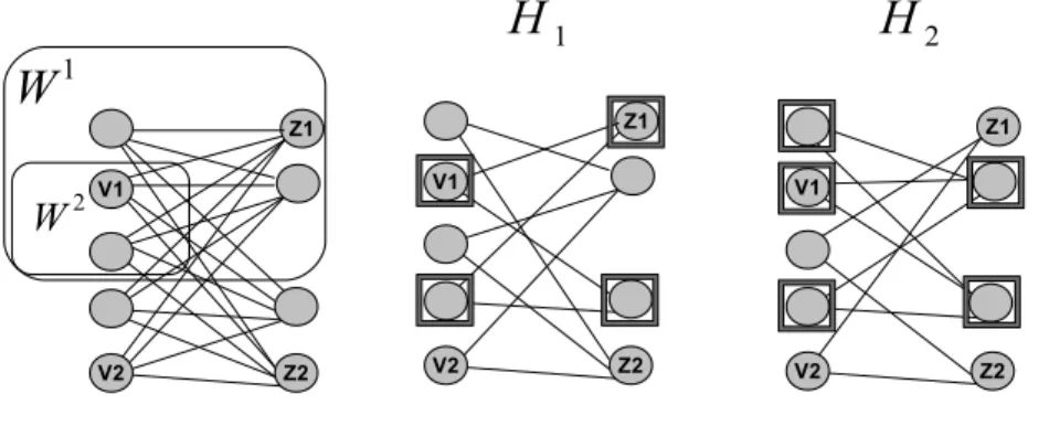
– Case W2 ⊆ (W1∩ V
1) or (W1 ∩ V1) ⊆ W2. One of the two connected
components of the graph Hδ(Wi)∆δ(U)corresponds to the node set {v1, z1}∪ (V1\ (W1∪ {v2})) ∪ (V2\ (W1∪ {z2})) for i = 1 and to the node set
{v1} ∪ (V1\ (W2∪ {v2})) ∪ (V2\ {z1, z2}) for i = 2.
Fig. 2 Illustration for the proof of Proposition 7 on the graph K5,4: case W2⊆ (W1∩ V1)
or (W1∩ V
1) ⊆ W2.
3 On the diameter of uniform cut polytopes
In this section we start dealing with some simple cases illustrating when the diameters of the cut and uniform cut polytopes may coincide or differ. We then express necessary and sufficient conditions for the incidence vectors of two cuts to be adjacent on a uniform cut polytope.
3.1 Particular cases 3.1.1 Complete graphs
A consequence of Theorem 1 is that any two different cuts in a complete graph have incidence vectors which are adjacent on CU T (Kn), i.e. the cut polytope
CU T (Kn) has diameter one. In particular, the incidence vectors of any two
different uniform cuts are adjacent, so that the latter property is ’inherited’ by uniform cut polytopes.
Corollary 4 For all integers n ≥ 1 and k ≤ ⌊n
2⌋, the uniform cut polytopes
CU T=k(Kn) have diameter 1.
3.1.2 Uniform cut polytopes with diameter 1
For a general graph G, both the general and uniform cut polytopes may have a diameter strictly larger than one. Consider for example the case when G consists of an elementary path with four nodes: (v1, v2, v3, v4). Then the
in-cidence vectors of the cuts δ(v2) and δ(v4) are not adjacent on CU T=1(G).
(This can be seen from the relation χδ(v2)+ χδ(v4)= χδ(v1)+ χδ(v3)). In fact, by Theorem 1 we have diameter(G) > 1 for any connected graph G = (V, E) with at least three nodes and that is not complete. (For, one may consider for
example the incidence vectors of the cuts δ(v) and δ(w) for two nonadjacent vertices v, w ∈ V ).
The following proposition gives a sufficient condition on G for the uniform cut polytope CU T=1(G) to have diameter 1.
Proposition 8 If G = (V, E) is a connected graph satisfying the following condition then the diameter of CU T=1(G) is 1. For each pair of nodes (i, j) ∈
V2 either:
– ij ∈ E, or
– there exists an elementary path in G joining i and j with length (= number of edges) at least 3, or
– all the elementary paths joining the nodes i and j have length 2 and either – min(deg(i), deg(j)) ≥ 2 and max(deg(i), deg(j)) ≥ 3, or
– all the nodes in N (i) ∩ N (j) have degree at least 3.
Proof We prove the proposition by exhibiting an edge-weight function w for each pair of nodes (i, j) ∈ V2 such that the incidence vectors of the cuts δ(i)
and δ(j) are the only two optimal solutions of the problem: maxv∈V w(δ(v)).
Case 1: ij ∈ E. Set wij:= 1 and we:= 0, ∀e ∈ E \ {ij}.
Case 2: There exists a path from i to j denoted (v0= i, v1, . . . , vl−1, vl= j)
with length l ≥ 3. Set wv0v1 := wvl−1vl := 1, wv1v2 := wvl−2vl−1 := −2, and a weight of value 0 for all the other edges.
Case 3: All the elementary paths in G joining the nodes i and j have length (= number of edges) 2 and either min(deg(i), deg(j)) ≥ 2 and max(deg(i), deg(j)) ≥ 3, or all the nodes in N (i) ∩ N (j) have degree at least 3. Set we:= deg(k)1 if
e ∈ δ(k) for k ∈ {i, j} and we:= −2 otherwise.
So as Theorem 1, Proposition 8 implies that for the case of a complete graph G the diameter of CU T=1(G) is 1. In addition, among others, Proposition
8 provides us with other family of graphs, namely the stars (or e.g. cycles) with at least 4 nodes, for which the diameter of the cut polytope (recall from Proposition 6 that the diameter of CU T (K1,p) with p ≥ 4 is p) is strictly
larger than that of the uniform cut polytope CU T=1(K1,p), p ≥ 4 (with value
1).
3.1.3 3-vertex connected graphs and connections with partition polytopes In this subsection we establish a simple upper bound on the diameter of uni-form cut polytopes of 3-vertex connected graphs and discuss some connections between the structures of uniform cut polytopes and partition polytopes for this graph family.
Recall that a graph G = (V, E) is said to be k-vertex connected if, for any node subset Q ⊆ V with cardinality |Q| < k, the node induced subgraph G[V \ Q] is connected. The next proposition is a consequence of Proposition 12 that we prove later.
Corollary 5 If the graph G is 3-vertex connected then the incidence vectors of the cuts δ(S ∪ {v}) and δ(S ∪ {w}) are adjacent on CU T=k(G), ∀S ⊆ V
with |S| = k − 1, and ∀v, w ∈ V \ S.
Proof Setting C1 := {v}, C2 := {w} and using the 3-vertex connectivity of
the graph G, the assumptions of Proposition 12 are satisfied.
It directly leads to the following upper bound on the diameter of uniform cut polytopes for 3-vertex connected graphs.
Proposition 9 If the graph G is 3-vertex connected, then diameter(CU T=k(G)) ≤ k.
Remark. We may establish some connections between the 1-skeletons of uni-form cut polytopes and bipartition polytopes. The bipartition polytope BP (k, n), with k, n ∈ N, k ≤ ⌊n2⌋, (a special case of the partition polytope [3,7]) is for-mally defined as the set of vectors y = (y1, y2) ∈ Rn× Rn satisfying the
following constraints n X j=1 y1 j = k (1) n X j=1 yj2= n − k (2) yj1+ yj2= 1, ∀j ∈ {1, . . . , n} (3) y ∈ R2n +. (4)
Bipartition polytopes arise in problems where the aim is to divide a set of n items into two sets of prescribed sizes: k and n − k. So, differently from the uniform cut polytope there is no underlying graph structure that is as-sociated with the items and it is (a (n − 1)-dimensional polytope) expressed in R2n (while in R|E| for CU T
=k(G) with G = (V, E)). Also as the matrix
corresponding to the constraints (1)-(4) is totally unimodular, it corresponds to an explicit description of the convex hull of the incidence vectors of bi-partitions having one part with cardinality k (and the other with cardinality n − k), whereas such an explicit description is unknown for general uniform cut polytopes.
The following proposition (see, e.g., Lemma 5 in [2] which corresponds to an extension of this result for more general partition polytopes) gives a characterization of the adjacency relation between vertices of the bipartition polytope.
Proposition 10 The incidence vectors of the two bipartitions (S1, V \S1) and
(S2, V \ S2) with S1, S2⊆ V , |S1| = |S2| = k ≤ |V |2 (if k = |V |2 then the set S2
defining the second partition is chosen such that |S1∩ S2| ≥ |S1∩ (V \ S2)|) are
adjacent on the 1-skeleton of the bipartition polytope BP (k, n) if and only if the sets S1and S2differ in exactly one item, i.e. there exists (v1, v2) ∈ S1×(V \S1)
Now let GP = (VP, EP) (resp. GC = (VC, EC)) denote the graph
cor-responding to the 1-skeleton of the bipartition polytope BP (k, n) (resp. of the uniform cut polytope CU T=k(G)), with n = |V |, G = (V, E) 3-vertex
connected.
Consider the application Ψ : VP → VC, which to any vertex v 1 ∈ VP
corresponding to the bipartition (X1, V \ X1) with |X1| = k, associates the
vertex Ψ (v1) ∈ VC corresponding to the cut δ(X1).
By Corollary 5 and Proposition 10 it follows that if (v1, v2) ∈ EP then
either Ψ (v1) = Ψ (v2) or (Ψ (v1), Ψ (v2)) ∈ EC. And as each vertex in VC is the
image of at least one vertex of VP by Ψ , this namely implies that the graph
GC may be obtained from GP by merging nodes and adding edges. Thus the
following inequality holds
diameter(CU T=k(G)) ≤ diameter(BP (k, n)) = k (5)
where G stands for any 3-vertex connected graph with order n (see, e.g. Corol-lary 6 in [2] for the last equality and Theorem 5 in the same reference for further results on the diameter of more general partition polytopes). ⋄
3.2 Necessary and sufficient conditions for adjacency on uniform cut polytopes
In this section we formulate necessary and sufficient conditions for the inci-dence vectors of two cuts to be adjacent on a uniform cut polytope CU T=k(G)
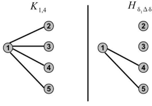
since in general, the characterization of adjacency between the incidence vec-tors of cuts as is given by Theorem 1 for the general cut polytope, does not hold for uniform cut polytopes. For, we may start giving an elementary ex-ample to illustrate this by considering a star on five nodes, see Figure 3. The two cuts we consider are δ1 = δ({1, 2}) and δ2 = δ({1, 3}). Both graphs G
and Hδ1∆δ2 (as defined in Theorem 1) are depicted. Since Hδ1∆δ2 contains three connected components the incidence vectors of these two cuts are not adjacent on the cut polytope CU T (G). Consider now the following cost func-tion defined on the edges of G: w12 = w13 = 1 and w14 = w15 = 2. Then we
can easily check that the only cuts solving the following optimization prob-lem: maxS⊆V (G) : |S|=2w(δ(S)) are δ1 and δ2, and thus they are adjacent on
CU T=2(G).
3.2.1 A necessary condition for adjacency on uniform cut polytopes
We now formulate a necessary condition for two incidence vectors of cuts in CU T=k(G) to be adjacent. For, we start introducing some notation and
terminology. Let Ci ⊆ V and δi = δ(Ci), with |Ci| = k, for i = 1, 2. Given a
node set W ⊆ V , the cuts δ1and δ2will be said to coincide (resp. be opposed)
on W if C1∩ W = C2∩ W (resp. C1∩ W = W \ C2).
Let I denote an index set on the connected components of the graph Hδ1∆δ2. To each connected component of Hδ1∆δ2 corresponding to a set of
Fig. 3 An illustration for the case of two cuts with incident vectors that are adjacent on the uniform cut polytope CU T=2(G) but not on CU T (G)
vertices Ai ⊆ V , i ∈ I, we can associate a bipartition (Vi
1, V2i) of Ai with
Vi
1 = C1∩ Ai. For each i ∈ I, we have the property that the cuts δ1 and
δ2 either coincide or are opposed on Ai (this follows from the definition of
Hδ1∆δ2).
Let I ⊆ I denote the index set on the connected components of Hδ1∆δ2 on which δ1 and δ2 are opposed. We can then express a necessary condition for
δ1and δ2 to be adjacent on a uniform cut polytope as follows.
Proposition 11 With the sets δ1, δ2, V1i, V2i, I, I as defined above, if the
inci-dence vectors of the cuts δ1and δ2are adjacent on CU T=k(G) then there does
not exist any set I′⊆ I with I 6= I′6= I such that P
i∈I′|V1i| = Pi∈I′|V2i| and
P
i∈I′∩I|V2i| + Pi∈I′\I|V1i| = Pi∈I′∩I|V1i| + PI′\I|V2i|.
Proof By contradiction. For, assume there exists I′ 6= I such that P
i∈I′|V1i| =
P
i∈I′|V2i| and Pi∈I′∩I|V2i| + Pi∈I′\I|V1i| = Pi∈I′∩I|V1i| + PI′\I|V2i|. Then
consider the two cuts δ(Ci′) with Ci′ ⊆ V , i = 1, 2, defined as follows:
– C′
1:= (∪i∈I\I′V1i) ∪ (∪i∈I′V2i), – C′
2:= (∪i∈I\(I∆I′)V1i) ∪ (∪i∈I∆I′V2i).
By the definition of the sets Cj, (Vji)i∈I, for j = 1, 2 and the assumption made
on the set I′, we have |C′
1| = |C2′| = k. Then observe that for an edge
– e ∈ δ1∩ δ2, we have e ∈ δ(C1′) ∩ δ(C2′),
– e /∈ δ1∪ δ2, we have e /∈ δ(C1′) ∪ δ(C2′),
– e ∈ δ1\ δ2 we can write e = vivj∈ Ai× Aj with (i, j) ∈ (I \ I) × I, i 6= j,
and either j ∈ I \ I′, e ∈ δ(C′
1) or j ∈ I ∩ I′, e ∈ δ(C2′),
– e ∈ δ2\ δ1, we can proceed as in the case before, showing it belongs either
to δ(C′
1) or δ(C2′).
It follows that χδ1+ χδ2 = χδ(C1′)+ χδ(C2′), implying that χδ1 and χδ2 are not adjacent on CU T=k(G).
Roughly speaking, the two conditions in Proposition 11 express the fact that it is not possible to permute a subset of the vertices in one shore of the cut δ1 = δ(C1) (or δ2 = δ(C2)) with a subset of vertices in the other
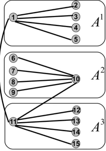
shore, such that the cardinality of the resulting shores is unchanged and the set of vertices permuted corresponds to the union of connected components in Hδ1∆δ2. We provide a simple example in Figure 4 illustrating the fact that the condition expressed in Proposition 11 (and in particular the second equation) is necessary for the incidence vectors of the cuts δ1 and δ2 to be adjacent on
CU T=k(G). In this example we consider cuts having one shore with cardinality
k = 6. Let C1 = {1, 6, 7, 8, 9, 11}, and C2 = {2, 3, 4, 5, 10, 11} define the cuts
δi= δ(Ci) for i = 1, 2. The figure represents the graph G and indicates the sets
of vertices (Ai)3
i=1 corresponding to the connected components of Hδ1∆δ2. We have I = {1, 2} and δ1∆δ2= {(1, 11), (10, 11)}. Considering the following edge
cost function: ce= 0 if e ∈ δ1∆δ2and ce= 1 otherwise, we can check that there
exist 3 cuts of maximum value in CU T=6(G) w.r.t. this cost function: δ1, δ2
and δ3= δ({1, 10, 12, 13, 14, 15}). So the incidence vectors of these cuts define
a face of dimension 2 of this polyhedron (since they are affinely independent) and they are all adjacent on CU T=6(G). Considering the index set I′ = {2, 3},
this illustrates the need for the satisfaction of the two conditions formulated in Proposition 11 (in this example I′ violates the second equation).
Fig. 4 Illustration for Proposition 11.
We terminate our discussion on Proposition 11 by giving an example show-ing that the given necessary condition is generally not sufficient for two cuts to
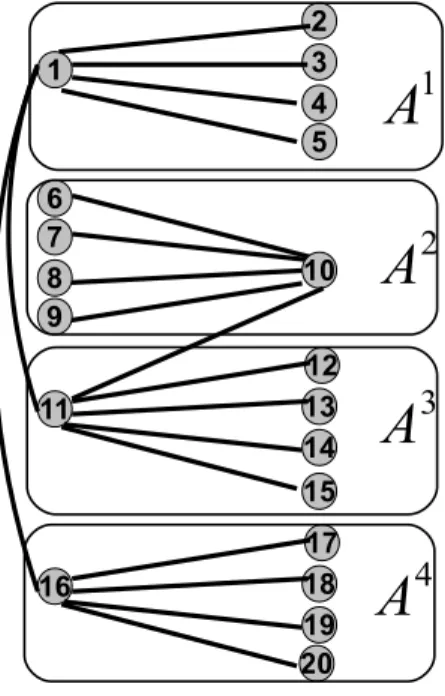
have their incidence vectors adjacent on a uniform cut polytope. The graph G is displayed in Figure 5, and we consider the uniform cut polytope CU T=7(G).
The figure also represents the node sets (Ai)4
i=1 which correspond to the
con-nected components of the graph Hδ1∆δ2 with δ1= δ({1, 6, 7, 8, 9, 11, 16}) and δ2 = δ({2, 3, 4, 5, 10, 11, 16}). So in this example we have I = {1, 2} and
the only two possibilities for a set I′ 6= I, I′ ⊆ I such that P
i∈I′|V1i| =
P
i∈I′|V2i| are {2, 3} and {2, 4} and none verifies Pi∈I′∩I|V2i|+Pi∈I′\I|V1i| =
P
i∈I′∩I|V1i|+PI′\I|V2i|. So the necessary condition expressed by Proposition
11 is satisfied. But considering now the cuts δ3 = δ({1, 10, 12, 13, 14, 15, 16})
and δ4= δ({1, 10, 11, 17, 18, 19, 20}), we have χδ1+ χδ2 = χδ3+ χδ4, implying
that χδ1 and χδ2 are not adjacent on CU T
=7(G).
Fig. 5 Illustration for the fact that Proposition 11 does not provide a characterization for the adjacency relation on uniform cut polytopes.
3.2.2 Sufficient conditions for adjacency on uniform cut polytopes
The following proposition, which straightforwardly follows from Theorem 1, formulates a simple sufficient condition for the incidence vectors of two cuts to be adjacent on a uniform cut polytope. It corresponds to the adjacency relations on the uniform cut polytopes which are ”inherited” from those on the cut polytope CU T (G).
Corollary 6 Let G = (V, E) be a connected graph and let (C1, C2, S, W )
de-note a partition of V such that |C1| = |C2| 6= 0, |C1| + |S| = k, G[C1∪ C2]
and G[S ∪ W ] are connected. Then the incidence vectors of the cuts δ(S ∪ C1)
and δ(S ∪ C2) are adjacent on CU T=k(G).
We formulate hereafter further sufficient conditions for the incidence vec-tors of two cuts to be adjacent on a uniform cut polytope.
The next one may be applied to the example illustrated in Figure 3 to prove adjacency of the two cuts mentioned there (whereas Corollary 6 cannot be applied for that case). It can be proved in a similar manner. We give the proof for completeness.
Proposition 12 Let G = (V, E) be a connected graph and let (C1, C2, S, W )
denote a partition of V such that |C1| = |C2| 6= 0, |C1| + |S| = k, G[C1], G[C2]
and G[S ∪ W ] are connected. Then the incidence vectors of the cuts δ(S ∪ C1)
and δ(S ∪ C2) are adjacent on CU T=k(G).
Proof The case when G[C1∪ C2] is connected follows from Corollary 6, and
so we may assume that G[C1∪ C2] is not connected whereas G[C1] and G[C2]
are.
Let T denote a tree on the graph G and consider the following edge cost function ce= 1 if e ∈ T ∩ δ(S ∪ C1) ∩ δ(S ∪ C2) −1 if e ∈ E \ (δ(S ∪ C1) ∪ δ(S ∪ C2)) 0 otherwise.
Then the only integer solutions for the optimization problem max{ctx : x ∈
CU T=k(G)} are the incidence vectors of the cuts δ(S ∪ C1), δ(S ∪ C2) and
possibly δ(W ) (the latter case may occur only if |W | = k), with objective value |T ∩ δ(S ∪ C1) ∩ δ(S ∪ C2)|. Thus the incidence vectors of the two cuts
δ(S ∪ C1) and δ(S ∪ C2) are adjacent on CU T=k(G).
A similar reasoning (based on connectivity properties of the graph Hδ1∆δ2) leads to the next two propositions giving other sufficient conditions for adja-cency on the 1-skeleton of uniform cut polytopes. Their proofs is similar to that of Proposition 12 and hence omitted.
Proposition 13 Let G = (V, E) be a connected graph and let (C1, C2, W )
denote a partition of V such that |C1| = |C2| = k, G[C1] is connected and
all connected components of G[W ] have cardinality at least k + 1 (or possibly, there is a single connected component with cardinality k and all the others with a strictly larger cardinality). Then the incidence vectors of the cuts δ(C1) and
δ(C2) are adjacent on CU T=k(G).
Proposition 14 Let G = (V, E) be a connected graph. If the graph Hδ1∆δ2 with δi = δ(Ci), Ci ⊆ V and |Ci| = k for i = 1, 2 has at most one connected
component with cardinality lower than or equal to 2k, then the incidence vec-tors of the cuts δ1 and δ2 are adjacent on CU T=k(G).
We end this section with another formulation of a sufficient condition for the adjacency on uniform cut polytopes. As Proposition 12 it may be applied to the example that is illustrated by Figure 3. We first introduce some no-tation. Given two incidence vectors of cuts in CU T=k(G): δj = δ(Cj), with
|Cj| = k (k ≤ ⌊n2⌋) for j = 1, 2, we denote by (Ai)mi=1 the sets of vertices
corresponding to the connected components of the graph Hδ1∆δ2 and we set i∗:= Argmax
i=1,...,m(minj=1,2|Ai\ Cj|).
Proposition 15 With the notation above, if the graph G is connected and the cuts δ1 and δ2, δ16= δ2 are such that
i) Hδ1∆δ2 has three connected components, ii) minj=1,2|Ai
∗
\ Cj| ≥ k
iii) ∃i ∈ {1, 2, 3} \ {i∗} such that |Ai∩ C
1| 6= |Ai∩ C2|
then the incidence vectors of the cuts δ1 and δ2 are adjacent on the polytope
CU T=k(G).
Proof For simplicity in the presentation and without loss of generality assume that the node sets (Ai)3
i=1 corresponding to the three connected components
of Hδ1∆δ2 are such that i
∗ = 3 and |A1∩ C
1| 6= |A1∩ C2|. (For the example
mentioned in Figure 3, one may take A1= {2}, A2= {3}, A3= {1, 4, 5}).
Claim 1. We have: Ck∩ (A1∪ A2) 6= ∅, ∀k ∈ {1, 2}.
Proof of Claim 1. We do the proof for k = 1 (the case k = 2 is symmetric). The proof we give is by contradiction. Assume that C1∩ (A1∪ A2) = ∅. Then
C1 ⊆ A3. Also note that for each connected component Ai in Hδ1∆δ2, the nodes in Ai can be partitioned into two node sets (Vi
1, V2i) such that each
set Vi
k (for k = 1, 2) is contained in one of the shores of the cuts δ1 and δ2.
With this observation it follows that necessarily C2= A3\ C1 (a consequence
of property (ii), the definition of the graph Hδ1∆δ2 and the assumption that δ16= δ2∈ CU T=k(G)). But then we get a contradiction with iii). ⋄
Note that a consequence of the claim to be used later is that C1∩ A3 =
C2∩ A3.
Now, let T denote a tree on the graph G and consider the following edge cost function: ce= 1 if e ∈ T ∩ δ1∩ δ2 −1 if e ∈ E \ (δ1∪ δ2) 0 otherwise.
Then the incidence vectors of the cuts δ1 and δ2 are optimal solutions for
the problem max{ctx : x ∈ CU T
=k(G)} with objective value |T ∩ δ1∩ δ2|.
And notice that any other different optimal solution corresponding to the incidence vector of a cut δ(C), |C| = k must verify either C ∩ A3 = C
1∩ A3
or C ∩ A3 = A3\ C
1. The latter case can occur only if |A3\ C1| = k (using
assumption (ii)) and in that case there exists a unique optimal cut δ(C), |C| = k in CU T=k(G) that is optimal w.r.t. the edge cost function c and such
that C ∩ A36= C
Consider now a cut δ(C), |C| = k that is optimal w.r.t. the edge cost function c and such that C ∩ A3= C
1∩ A3.
Then, from the observation reported above and iii) it cannot differ from both δ1 and δ2.
It follows that under the conditions formulated in the proposition there exist at most three extreme points of CU T=k(G) which correspond to optimal
solutions w.r.t. the edge cost function c, among which the incidence vectors of the cuts δ1and δ2. It then follows that the latter are adjacent on CU T=k(G).
We give in Figure 6 an example where Proposition 15 can be used to show that two cuts are adjacent on a uniform cut polytope. The figure displays the graph G and the connected components (Ai)3
i=1 of the graph Hδ1∆δ2 for the cuts δ1 = δ({1, 4, 5, 7}) and δ2 = δ({2, 3, 6, 7}) of CU T=4(G). Notice that
Corollary 6 and Propositions 12, 13 and 14 do not apply here.
Fig. 6 Illustration for an example to which Proposition 15 may be applied to prove the adjacency of the incidence vectors of two cuts on a uniform cut polytope.
References
1. F. Barahona and A.R. Mahjoub, On the cut polytope, Mathematical Programming, 36:2, 157–173 (1986)
2. S. Borgwardt, On the diameter of partition polytopes and vertex-disjoint cycle cover, Mathematical Programming (2011)
3. J.A. De Loera, Transportation polytopes: a twenty year update. University of California, Davis. Slides of talk at Workshop on Convex Sets and their Applications. Banff (2006) 4. M.M. Deza and M. Laurent, Geometry of Cuts and Metrics, Algorithms and
Combina-torics, vol. 15, Springer, Berlin (1997)
5. M.R. Garey and D.S. Johnson, Computers and Intractability: A Guide to the Theory of NP-Completeness. W. H. Freeman (1979)
6. B. Gr¨unbaum, Convex Polytopes, Springer, 2nd ed., New York (2003)
7. V. Klee and C. Witzgall, Facets and vertices of transportation polytopes. In Dantzig, G.B., Veinott, A.F. (eds) Mathematics of the Decision Sciences, vol.1 257–282 (1968) 8. T. Matsui and S. Tamura, Adjacency on combinatorial polyhedra. Discrete Applied
Mathematics 56, 311–321 (1995)
9. D. Naddef and W.R. Pulleyblank, Hamiltonicity and Combinatorial Polyhedra. Journal of Combinatorial Theory, Series B 31, 297–312 (1981)
10. D. Naddef, The Hirsch conjecture is true for (0,1)-polytopes. Mathematical Program-ming 45, 109–110 (1989)
11. G. Ziegler, Lectures on Polytopes. Springer. Series: Graduate Texts in Mathematics, Vol. 152. (1995)