Rift Valley fever: An open-source transmission
dynamics simulation model
Robert Sumaye1,2,3☯
, Famke Jansen2☯
, Dirk Berkvens2, Bernard De Baets4,
Eveline Geubels1, Etienne Thiry3, Meryam KritID2*
1 Ifakara Health Institute, Ifakara, Tanzania, 2 Institute of Tropical Medicine, Department of Biomedical Sciences, Antwerp, Belgium, 3 University of Liège, Faculty of Veterinary Sciences, Liège, Belgium, 4 Ghent University, Faculty of Bioscience Engineering, Department of Data Analysis and Mathematical Modelling, Ghent, Belgium
☯These authors contributed equally to this work.
Abstract
Rift Valley fever (RVF) is one of the major viral zoonoses in Africa, affecting humans and several domestic animal species. The epidemics in eastern Africa occur in a 5-15 year cycle coinciding with abnormally high rainfall generally associated to the warm phase of the El
Niño event. However, recently, evidence has been gathered of inter-epidemic transmission.
An open-source, easily applicable, accessible and modifiable model was built to simulate the transmission dynamics of RVF. The model was calibrated using data collected in the Kilombero Valley in Tanzania with people and cattle as host species and Ædes mcintoshi, Æ. ægypti and two Culex species as vectors. Simulations were run over a period of 27 years using standard parameter values derived from two previous studies in this region. Our model predicts low-level transmission of RVF, which is in line with epidemiological studies in this area. Emphasis in our simulation was put on both the dynamics and composition of vec-tor populations in three ecological zones, in order to elucidate the respective roles played by different vector species: the model output did indicate the necessity of Culex involvement and also indicated that vertical transmission in Ædes mcintoshi may be underestimated. This model, being built with open-source software and with an easy-to-use interface, can be adapted by researchers and control program managers to their specific needs by plugging in new parameters relevant to their situation and locality.
Introduction
Rift Valley fever (RVF) is caused by the Rift Valley fever virus (RVFv), which belongs to the genusPhlebovirus in the family Bunyaviridae. RVF is one of the major viral zoonoses in Africa,
affecting man and several domestic animal species [1,2].
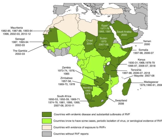
A syndrome compatible with RVF was first described in the Rift Valley of Kenya in the early 1900s and the virus was isolated in the 1930s [3]. The known range of RVFv is shown in
Fig 1. RVF was confined to eastern and southern Africa until about 1975. Since then it has expanded its range first to Egypt (1977), then to western Africa (ca. 1980) and finally to the a1111111111 a1111111111 a1111111111 a1111111111 a1111111111 OPEN ACCESS
Citation: Sumaye R, Jansen F, Berkvens D, De
Baets B, Geubels E, Thiry E, et al. (2019) Rift Valley fever: An open-source transmission dynamics simulation model. PLoS ONE 14(1): e0209929. https://doi.org/10.1371/journal.pone.0209929
Editor: Abdallah M. Samy, Faculty of Science, Ain
Shams University (ASU), EGYPT
Received: September 7, 2018 Accepted: December 13, 2018 Published: January 9, 2019
Copyright:© 2019 Sumaye et al. This is an open access article distributed under the terms of the Creative Commons Attribution License, which permits unrestricted use, distribution, and reproduction in any medium, provided the original author and source are credited.
Data Availability Statement: All relevant data are
within the manuscript and its Supporting Information files.
Funding: This work was supported by Robert
Sumaye’s PhD grant, obtained from the Belgian Directorate-General for Development Cooperation (DGD) within the Framework Agreement between DGD and ITM. The funders had no role in study design, data collection and analysis, decision to publish, or preparation of the manuscript.
Competing interests: The authors have declared
Arabian peninsula in 2000 [4]. It has so far not been officially confirmed from the Maghreb countries, although there is at least serological evidence of import into south-western Algeria [5], evidence of human exposure in Tunisia [6], mention of viral presence in Morocco, Algeria and Libya [7] and mention of exposure of camels, gazelle and water buffalo in Turkey [8]. Currently, an epidemic is being experienced in East Africa (Kenya, Rwanda, Tanzania and Uganda reporting cases in humans and animals, ProMED-mail, several postingshttp://www. promedmail.org). RVFv has been imported into countries outside the normal range, the most recent report being that of a patient, being diagnosed in China and having acquired the infec-tion in Angola [9].
The epidemics in eastern Africa and the Horn of Africa involve a 5–15 year cycle marked by abnormally high rainfall,e.g. during the warm phase of the El Niño/Southern Oscillation
phenomenon (ENSO) [10,11]. In other regions of Africa, the occurrence of the disease is
Fig 1. Geographical distribution of Rift Valley fever. The years indicate when the disease was detected in individual countries. Adapted from
CDC andhttps://www.nature.com/articles/emi201381/figures/1with supplementary information from [4–8]. Dark green: Chad, Egypt, Kenya, Madagascar, Mauritania, Mayotte (Fr.), Namibia, Saudi Arabia, Senegal, Somalia, South Africa, Sudan, Swaziland, Tanzania, The Gambia, Yemen, Zambia, Zimbabwe. Light green: Angola, Botswana, Burkina Faso, Cameroon, Central African Republic, Congo, Democratic Republic of the Congo, Ethiopia, Gabon, Guinea Conakry, Malawi, Mali, Mozambique, Niger, Nigeria, Rwanda, Uganda Light beige: Algeria, Libya, Morocco, Tunisia, Turkey.
linked to other sources of flooding,e.g. the construction of a hydroelectric dam along the
Sene-gal river [12,13].
In the past, the above was the traditional view of the epidemiology of RVF, but recently there is more and more evidence of so-called inter-epidemic transmission: previously unno-ticed low-level viral transmission in all species involved [12,14–18]. In Tanzania, human involvement in RVF inter-epidemic transmission has been reported in the past [19,20]. Dur-ing the 2006/07 RVF epidemic in eastern Africa, livestock and people in the Kilombero valley in Tanzania were affected [21]. Two serological surveys in this region since this last epidemic, one in livestock and one in people, effectively showed the presence of inter-epidemic transmis-sion in the area [17,22].
RVF is transmitted to humans and other mammalian hosts, both livestock and wild rumi-nants (e.g. cattle, buffalo, sheep, goats and camels) through mosquito (e.g. Culex spp., Ædes
spp. andMansonia spp.) and other arthropod vector bites [1,2,16,23]. Ædine mosquitoes are capable of transovarial (= vertical) transmission of RVFv to the eggs, which can survive long droughts (several years) and hatch when new water arrives duringe.g. the ENSO phenomenon,
resulting in infected larvæ and adult mosquitoes [2]. The highest risk for humans to become infected is through direct and indirect contact with infectious animal materials (blood, body fluids or tissues of viræmic animals). Ærosol formation duringe.g. milking or consumption of
raw milk, meat or blood form another risk for transmission [13,24–28]. An established treat-ment method or a vaccine for humans currently does not exist. Control of the disease needs to be done through vaccination of livestock and preventive measures by humans [29,30].
Clinical manifestation in humans can go from only mild illness, including fever, muscle pain, joint pain and headache to severe forms with ocular disease, meningo-encephalitis or haemorrhagic fever [29,31]. The disease manifests itself in livestock through morbidity and mortality in newborns and abortions during all stages of the pregnancy. This has devastating effects on livestock populations and has severe economic repercussions for livestock keepers [2,26,32,33].
Quantitative analysis and simulation modelling of RVFv dynamics have been undertaken on several occasions. Note that the list that follows cites only typical examples and that many more publications exist dealing with RVF modelling. The analytical models use environmental characteristics and range from post-hoc predictions of where outbreaks were to be expected during the 2006-2007 epidemic in East Africa [10] over statistical modelling in order to iden-tify landscape features related to RVFv transmission [34] to the identification of ranges of potential vectors [35]. Simulation models include temporal models using differential equations [36] with extensions to spatial components [37]. Risk analysis of introduction into new terri-tory (in casu The Netherlands) [38] has also been carried out. An overview of compartmental models, applied to the simulation of RVF dynamics, is provided by Danzetta and colleagues [39].
The existing models all suffer from being closed, inaccessible and specialised. The combina-tion of R/RStudio1with the libraries shiny and deSolve offers the possibility to develop open-source, easily applicable, accessible and modifiable models that can, on the one hand, be adapted to a specific situation with minimal programming effort and, on the other hand, be perused by the epidemiological researcher to study different scenarios and/or the effects of dif-ferent parameter settings. The model presented here has been developed for the specific situa-tion in East Africa, but as explained above, it can easily be adapted to other areas/situasitua-tions, mostly by switching on or off certain parameters or parameter groups or by the inclusion of extensions with minimal new coding. The model presented in this paper is thus to be consid-ered a research tool, allowing the user to study the effect(s) of different scenarios in order to better understand RVFv transmission dynamics and the mammalian hosts and arthropod
vectors involved, and ultimately to assist in the formulation of new research questions. The model is not a predictive tool, as too much uncertainty still exists with regards to the actual dynamics of inter-epidemic transmission of the virus.
Model—General description
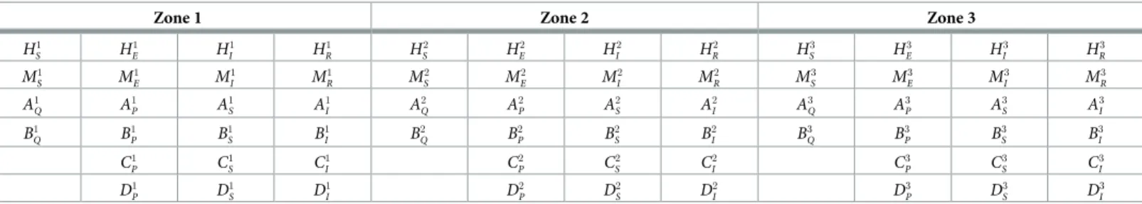
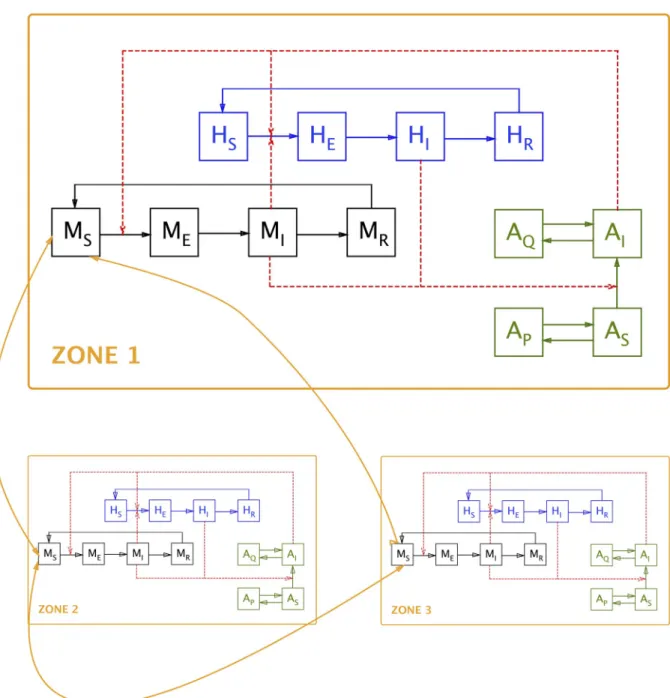
The model describes the RVFv transmission dynamics in six species (human population, domestic animal population and four vectors) in three different areas. The model attempts to offer maximal flexibility, whilst remaining manageable. The model allows for migration of the various species between the different areas. The different compartments in the model are pre-sented inTable 1and a simplified schematic representation of the model is shown inFig 2.
Each human and animal population consists of a susceptibleS, exposed E, infective I and
removedR (= recovered/immune) compartment. There is a flow back from the removed to
the susceptible compartment in both populations,i.e. immunity is not lifelong. All individuals
are born susceptible and a proportion of the pregnant infected animals abort. VectorsA and B
allow for vertical transmission: infected females (I compartment) transmit infection to their
eggs (Q compartment), where the virus survives until the larvæ hatch and the resulting adults
are infective. VectorA furthermore has the possibility of long-term dormancy in the egg stage
(both infected and non-infected).
A challenge lies in the correct modelling of the vector dynamics. More specifically, a point of attention is the distribution of feeding individuals over the different host populations (both species-wise and zone-wise). Vectors can feed on the two modelled host species (human and domestic animal), but they can also use alternative hosts (especially so in the forest zone). The latter means there is no increased mortality in case the two main hosts are not available, but this of course also influences infection prevalence in the vector population. The vector popula-tions are furthermore limited by a density-dependent oviposition rate. The approach currently taken uses the following basic parameters (see Vector feeding and infection rates for details): • ε: proportion of vector X feeding on host Λ in zone i; it is the user’s responsibility to ensure
that the sum of the variousε per species per zone does not exceed one
• η: (maximum) number of successful bites per time unit of vector X on host Λ
• πuv: probability to transmit infection from speciesu to species v (v 6¼ u) upon a successful
bite
• Oalt: number of alternative hosts
Table 1. Different compartments in the model.
Zone 1 Zone 2 Zone 3
H1 S H 1 E H 1 I H 1 R H 2 S H 2 E H 2 I H 2 R H 3 S H 3 E H 3 I H 3 R M1 S M 1 E M 1 I M 1 R M 2 S M 2 E M 2 I M 2 R M 3 S M 3 E M 3 I M 3 R A1 Q A 1 P A 1 S A 1 I A 2 Q A 2 P A 2 S A 2 I A 3 Q A 3 P A 3 S A 3 I B1 Q B 1 P B 1 S B 1 I B 2 Q B 2 P B 2 S B 2 I B 3 Q B 3 P B 3 S B 3 I C1 P C 1 S C 1 I C 2 P C 2 S C 2 I C 3 P C 3 S C 3 I D1 P D 1 S D 1 I D 2 P D 2 S D 2 I D 3 P D 3 S D 3 I
H = People; M = Domestic animals; A = Vector A; B = Vector B; C = Vector C; D = Vector D;
□S= susceptible;□E= exposed;□I= infective;□R= removed;
□Q= infected eggs;□P= non-infected eggs;
□1= Zone 1;□2= Zone 2;□3= Zone 3
• kjX: maximum number of vector X individuals in zonej (‘carrying capacity’)
El Niño events are currently modelled to occur every ten years. Additionally, the user is given the opportunity to include annual overall climate variability through the choice of a ran-dom series of ‘dry’ or ‘wet’ years and a seasonal within-year variation in egg eclosion to model seasonal effects on vector population size. Finally, there is the possibility of including a ‘fixed’ annual domestic animal movements between zones 1 and 2, simulating seasonal transhumance of (e.g.) cattle between the plateau and the floodplain. Details are to be found in Seasonality
and El Niño effect.
Fig 2. Diagrammatic representation of the model. Note: for the sake of clarity, inter-zone movement is indicated only for the susceptible
animal compartment (MS); it is identical for all other compartments. Also for the sake of clarity, compartments are only shown for human
population (H), domestic animal population (M) and one vector species (A); seeTable 1for a list of all compartments. https://doi.org/10.1371/journal.pone.0209929.g002
It is understood that the necessary calculations for these density-dependent oviposition-feeding, climatic variability and transhumance processes slow down the model considerably. It was therefore decided to rewrite part of the code, doing the preparatory computations before calling the deSolve routines (using the classical Runge-Kutta 4thorder method), in C++ (making use of the RCCP library). This speeds up execution by a factor of about sixty, but of course means a lower accessibility of the code. Therefore, a slower version, entirely written in R is also offered. Full details on how to install and run the model are given in the accompa-nying user’s manualS1 Appendix. The R and C++ code is provided inS2 Appendix.
Model—Differential equations
For every zonei(i = 1, 2, 3), we compute the differential equations of each compartment of the
human, the animal and the vector populations.
Human population
dHi S dt ¼ gHN i Hþ X3 j ¼ 1 j 6¼ i ljiHHSjþ rHH i R ðmHþ b i Hþ X3 j ¼ 1 j 6¼ i lijHÞHi S; ði ¼ 1; . . . ; 3Þ ð1Þ dHi E dt ¼ b i HH i Sþ X3 j ¼ 1 j 6¼ i ljiHHEj ðmHþ xHþ X3 j ¼ 1 j 6¼ i lijHÞHi E; ði ¼ 1; . . . ; 3Þ ð2Þ dHi I dt ¼ xHH i Eþ X3 j ¼ 1 j 6¼ i ljiHHjI ðmHþ dHþ aHþ X3 j ¼ 1 j 6¼ i lijHÞHi I; ði ¼ 1; . . . ; 3Þ ð3Þ dHi R dt ¼ aHH i Iþ X3 j ¼ 1 j 6¼ i ljiHH2 R ðmHþ rHþ X3 j ¼ 1 j 6¼ i lijHÞHi R; ði ¼ 1; . . . ; 3Þ ð4ÞEq 1describes the rate of change in the susceptible human compartment in Zonei: gHNiH
refers to the newborn individuals, P 3
j ¼ 1 j 6¼ i
ljiHHSjþ rHHiRrefers to the immigration into Zonei
from the other two zones and individuals losing their immunity while ðmHþ biHþ P 3
j ¼ 1 j 6¼ i
lijHÞHi S
refers to the losses through natural mortality, people becoming infected and emigration out of Zonei.Eq 2describes the rate of change in the human exposed (incubating) compartment in Zonei: biHHSi refers to the individuals having become infected,
P3
j ¼ 1 j 6¼ i
ljiHHjErefers to immigration
into zonei and mHþ xHþ
P3
j ¼ 1 j 6¼ i
lijHÞHi
Erefers to the losses through natural mortality, changing
from incubation to the infective stage and emigration from Zonei.Eq 3describes the rate of change in the infective human compartment: xHHi
Erefers to the individuals having become
infective, P 3 j ¼ 1 j 6¼ i lji HH j
Irefers to the immigration into Zonei and ðmHþ dHþ aHþ
P3 j ¼ 1 j 6¼ i lij HÞH i I
refers to the losses through natural mortality, disease-specific mortality, recovery and emigra-tion from Zonei.Eq 4describes the rate of change in the recovered (immune) human com-partment: aHHi
Irefers to individuals having recovered (gained immunity),
P3
j ¼ 1 j 6¼ i
ljiHH2
Rrefers to
immigration into Zonei and ðmHþ rHþ
P3
j ¼ 1 j 6¼ i
lijHÞHi
Rrefers to losses through natural mortality,
loss of immunity and emigration from Zonei.
Animal population
dMi S dt ¼ gMUN i Mþ gMIM i I � � 1 N i M ki M � � þX 3 j ¼ 1 j 6¼ i ljiMMSj þ rMM i R ðmMþ b i Mþ X3 j ¼ 1 j 6¼ i lijMÞMi S; ði ¼ 1; . . . ; 3Þ ð5Þ dMi E dt ¼ b i MM i Sþ X3 j ¼ 1 j 6¼ i ljiMMjE ðmMþ xMþ X3 j ¼ 1 j 6¼ i lijMÞMi E; ði ¼ 1; . . . ; 3Þ ð6Þ dMi I dt ¼ xMM i Eþ X3 j ¼ 1 j 6¼ i ljiMMIj ðmMþ dMþ aMþ X3 j ¼ 1 j 6¼ i lijMÞMi I; ði ¼ 1; . . . ; 3Þ ð7Þ dMi R dt ¼ aMM i Iþ X3 j ¼ 1 j 6¼ i ljiMMjR ðmMþ rMþ X3 j ¼ 1 j 6¼ i lijMÞMi R; ði ¼ 1; . . . ; 3Þ ð8ÞEq 5describes the rate of change in the susceptible animal host compartment: gM UN i Mþ gMIMIi � � 1 NMi ki M � �
refers to the newborn individuals, respectively born from unin-fected and inunin-fected individuals and corrected for population density to simulate removal (sales) in function of herd size, P
3
j ¼ 1 j 6¼ i
ljiMMSj þ rMMiRrefers to immigration into Zonei from the
other two zones and individuals losing their immunity and ðmMþ biMþP 3
j ¼ 1 j 6¼ i
lijMÞMi
Srefers to
losses through natural mortality, animals becoming infected and emigration out of Zonei.Eq 6describes the rate of change in the animal host exposed (incubating) compartment in Zonei:
biMMi
Srefers to the animals becoming infected,
P3
j ¼ 1 j 6¼ i
ljiMMjErefers to immigration into Zonei
and ðmMþ xMþ P 3
j ¼ 1 j 6¼ i
lijMÞMi
Erefers to the losses through natural mortality, changing from
incubation to the infective stage and emigration from Zonei.Eq 7describes the rate of change in the animal infective compartment in Zonei: xMMiErefers to the individuals becoming
infec-tive, P 3 j ¼ 1 j 6¼ i lji MM j
Irefers to the immigration into Zonei ands ðmMþ dMþ aMþ
P3 j ¼ 1 j 6¼ i lij MÞM i Irefers
to the losses through natural mortality, disease-specific mortality, recovery and emigration from Zonei.Eq 8describes the rate of change in the recovered (immune) animal compart-ment in Zonei: aMMi
Irefers to the animals having recovered (gained immunity),
P3
j ¼ 1 j 6¼ i
ljiMMRj
refers to immigration into Zonei and ðmMþ rMþ
P3
j ¼ 1 j 6¼ i
lijMÞMi
Rrefers to losses through natural
mortality, loss of immunity and emigration from Zonei.
Vector A
dAi Q dt ¼ o i AgA 1 Ni A ki A � � zAAi I ðm i AQþ tst i AÞA i Q; ði ¼ 1; . . . ; 3Þ ð9Þ dAi P dt ¼ gA 1 Ni A ki A � � oi Að1 zAÞA i Iþ ðo i Aþ o 1 A2ÞA i S h i mi APþ tst i A � � Ai P; ði ¼ 1; . . . ; 3Þ ð10Þ dAi S dt ¼ tst i AA i Pþ X3 j ¼ 1 j 6¼ i ljiAAjS ðmAþ o i Ab i Aþ X3 j ¼ 1 j 6¼ i lijAÞAi S; ði ¼ 1; . . . ; 3Þ ð11Þ dAi I dt ¼ tst i AA i Qþ o i Ab i AA i Sþ X3 j ¼ 1 j 6¼ i ljiAAjI ðmAþ X3 j ¼ 1 j 6¼ i lijAÞAi I; ði ¼ 1; . . . ; 3Þ ð12ÞEq 9describes the rate of change in the infected-egg compartment of Vector A in Zonei:
oi AgA 1 Ni A ki A � � zAAi
Irefers to the production of infected eggs (product of total biting rate,
egg production rate, density-dependent correction and vertical transmission rate) while ðmi
AQþ tst
i AÞA
i
Qrefers to losses through mortality and hatching (in function of El Niño and
sea-sonal flooding throughτs).Eq 10describes the rate of change in the uninfected-egg
compart-ment of Vector A in Zonei: gA 1 Ni A ki A � � oi Að1 zAÞAiIþ ðo i Aþ o 1 A2ÞA i S h i
refers to the density-dependence corrected production of uninfected eggs both by infected adult vectors (absence of vertical transmission) and uninfected adult vectors while ðmi
APþ tst
i AÞA
i
Prefers to losses
through mortality and hatching (in function of El Niño and seasonal flooding through τs).Eq
11describes the rate of change in the uninfected-adult-vector compartment in Zonei: tstiAAiP
refers to the newly ‘hatched’ adults (note that stages intervening between egg and adult are omitted, requiring adjustment of hatching and mortality rates), P
3
j ¼ 1 j 6¼ i
ljiAAjSrefers to the
immi-gration into Zonei and ðmAþ oiAb i Aþ P3 j ¼ 1 j 6¼ i lijAÞAi
Srefers to the losses through mortality,
acquisition of infection and emigration out of Zonei.Eq 12describes the rate of change in the infected-adult-vector compartment in Zonei: tstiAAiQrefers to the newly ‘hatched’
infected adult vectors (same remark as forEq 11), oi
Ab
i
vectors, P 3
j ¼ 1 j 6¼ i
ljiAAjIrefers to the immigration into Zonei and ðmAþ
P3
j ¼ 1 j 6¼ i
lijAÞAi
Irefers to the losses
through mortality and emigration out of Zonei.
Vector B
dBi Q dt ¼ o i BgB 1 Ni B ki B � � zBBi I ðm i BQþ tst i BÞB i Q; ði ¼ 1; . . . ; 3Þ ð13Þ dBi P dt ¼ gB 1 Ni B ki B � � oi Bð1 zBÞB i Iþ ðo i Bþ o i B2ÞB i S h i mi BPþ tst i B � � Bi P; ði ¼ 1; . . . ; 3Þ ð14Þ dBi S dt ¼ tst i BB i Pþ X3 j ¼ 1 j 6¼ i ljiBBjS ðmBþ o i Bb i Bþ X3 j ¼ 1 j 6¼ i lijBÞBi S; ði ¼ 1; . . . ; 3Þ ð15Þ dBi I dt ¼ tst i BB i Qþ o i Bb i BB i Sþ X3 j ¼ 1 j 6¼ i ljiBBjI ðmBþ X3 j ¼ 1 j 6¼ i lijBÞBi I; ði ¼ 1; . . . ; 3Þ ð16ÞThe differential equations describing the dynamics of Vector B are identical as those for Vector A, the only difference being the possible presence of dormant eggs in the latter and not in the former.
Vector C
dCi P dt ¼ gC 1 Ni C ki C � � oi CC i Iþ ðo i Cþ o i C2ÞC i S h i mi CPþ tstC � � Ci P; ði ¼ 1; . . . ; 3Þ ð17Þ dCi S dt ¼ tstCC i Pþ X3 j ¼ 1 j 6¼ i ljiCCjS ðmCþ o i Cb i Cþ X3 j ¼ 1 j 6¼ i lijCÞCi S; ði ¼ 1; . . . ; 3Þ ð18Þ dCi I dt ¼ o i Cb i CC i Sþ X3 j ¼ 1 j 6¼ i ljiCCjI ðmCþ X3 j ¼ 1 j 6¼ i lijCÞCi I; ði ¼ 1; . . . ; 3Þ ð19ÞVector C differs from Vectors A and B in the absence of vertical transmission and hence the absence of an infected-egg compartment (i.e. nodCiQ
dt differential equation). Infected adult
vectors can only originate through uninfected adults acquiring infection (oi Cb
i
CC
i
S) and there is
Vector D
dDi P dt ¼ gD 1 Ni D ki D � � oi DD i Iþ ðo i Dþ o i D2ÞD i S h i mi DPþ tstD � � Di P; ði ¼ 1; . . . ; 3Þ ð20Þ dDi S dt ¼ tstDD i Pþ X3 j ¼ 1 j 6¼ i lji DD j S ðmDþ oiDb i Dþ X3 j ¼ 1 j 6¼ i lij DÞD i S; ði ¼ 1; . . . ; 3Þ ð21Þ dDi I dt ¼ o i Db i DD i Sþ X3 j ¼ 1 j 6¼ i lji DD j I ðmDþ X3 j ¼ 1 j 6¼ i lij DÞD i I; ði ¼ 1; . . . ; 3Þ ð22ÞVector D is identical to Vector C.
Auxiliary equations
Population totals
Ni H¼H i SþH i EþH i IþH i R; ði ¼ 1; . . . ; 3Þ ð23Þ Ni M¼M i SþM i EþM i R; ði ¼ 1; . . . ; 3Þ ð24Þ Ni A¼A i QþA i PþA i SþA i I; ði ¼ 1; . . . ; 3Þ ð25Þ Ni B¼B i QþB i PþB i SþB i I; ði ¼ 1; . . . ; 3Þ ð26Þ Ni C¼C i PþC i SþC i I; ði ¼ 1; . . . ; 3Þ ð27Þ Ni D ¼D i PþD i SþD ; Iði ¼ 1; . . . ; 3Þi ð28ÞVector feeding and infection rates
Parameters29–35are the basic parameters used to compute carrying capacity etc. of a zone
vis-à-vis its resident vectors. The present approach is to compare the total number of bites
(successful feedings, . . .– for sake of brevity referred to as ‘bites’ from now on) the vectors can inflict upon the hosts per time unit with the total number of number of vector bites the host populations can sustain (given their resistance, evasive behaviour, . . .). The minimum value of these two is used to compute the actual number of bites given per vector and/or the number of bites suffered per host. It is understood that this approach may introduce a number of parame-ters whose values are only vaguely known at best, but an attempt was made to avoid unrealistic numbers of vectors interacting with a single host,i.e. host numbers determine vector numbers.
At the same time, the possibility is offered to include so-called alternative hosts, which can be used by the vectors when the hosts included in the model are insufficient, in order to avoid
vectors disappearing when host population levels are too low.
εkj¼proportion of vector population Xkfeeding on host Lj
X
j
εkj� 1Þ ð29Þ
nk ¼average number of bites an individual of vector Xkissues per time unit ð30Þ
Zj ¼maximum number of bites host Ljcan ‘sustain’ per time unit;
before e:g: taking evasive action or dislodging behaviour ð31Þ
φj0;j¼number of j 0
transmitting hosts contacted by receiving host j per time unit ð32Þ puv¼probability to transmit infection from u to v ð33Þ
with u 2 fj; kg & v 2 fk; jg & v 6¼ u ð34Þ
bwl¼probability to pick up infection from wildlife hosts in general ð35Þ Parameters36and37are computed from the simulation output:
NXk¼Population size of vector Xk ð36Þ
NLj ¼Population size of host Lj ð37Þ
The potential maximum number of vector bites (all vector species) on whole host popula-tionΛjis computed as:
Oj¼X
k
εkjNXknk ð38Þ
This is compared with the maximum number of bites the same host population can ‘sustain’ (see above for more details):
wj¼ ZjNLj ð39Þ
The ‘availability’ of host populationΛj(i.e. the proportion of the potential bites actual
inflicted on the host population in question) is the ratio of parameter39over parameter38
with a maximum of unity:
sj¼min 1;wj Oj
!
ð40Þ
The actual number of bites by vector Xkon the whole host populationΛjis thus:
Okj¼εkjNXknksj ð41Þ
The individual biting rate of vector Xkon hostΛjper time unit becomes:
The total individual biting rate of vector Xkon all host populations per time unit therefore is the sum of the respectiveωkj:
ok¼X
j
okj ð43Þ
The biting rate of vector Xkon alternative hosts (with Oalt= number of alternative hosts) is
defined as: ok 2¼ Oalt NXk ð44Þ
The proportion of infection in vector Xkfeeding on all modelled hosts species is computed
as (the reference to the zone is left out,ILjbeing the number of infective individuals of hostΛj;
βwlrefers to the infection picked up from game animals and it is added only in the case of
Zone-3-dwelling vectors): bk¼min 1;X j pjk ILj NLj þ bwl ! ð45Þ
The infection rate of hostΛjbeing subjected to the actual number of bites by the various
vectors and/or interacting with other infectious hosts is calculated as (φj0,jrefers to the number of transmitting hosts [domestic animal] met by one receiving host [a person] per time unit; Okj NLj IXk NXkbecomes okjIXk NLj because okj¼ Okj NXk): bj ¼ log 1 1 Y k ð1 pXkLjÞ okjIXk NLj 2 6 6 4 3 7 7 5 1 Y j0 ð1 pL j0LjÞ φj0;jILj0 NLj0 2 6 6 6 4 3 7 7 7 5 8 > > > < > > > : þ 1 Y k ð1 pXkLjÞ okjIXk NLj 2 6 6 4 3 7 7 5 � 1 Y j0 ð1 pLj0LjÞ φj0;jIL j0 NL j0 2 6 6 6 4 3 7 7 7 5 9 > > > = > > > ; 8j06¼j ð46Þ
The second and third terms of the logarithm function ofEq 46are currently implemented only for animal-to-human direct transmission.
Seasonality and El Ni
ño effect
Simulating an annual (seasonal) animal transhumance between Zone 1 and Zone 2 is possible: animals move to Zone 1 on dayd1and move back to Zone 2 on dayd2. This is achieved
through the generation of 0/1 indicators, which are to be multiplied with the movement rate:
l12M ¼ ½t � d1 ðmod 360Þ� ð47Þ
l21M ¼ ½t � d2 ðmod 360Þ� ð48Þ
Hatching of dormant eggs of Vector A can be regulated on a seasonal basis as well as peri-odically through El Niño events in Zone 1 (d3andd4are respectively the start and end of the
are respectively the start and end of the El Niño event): t1 A¼ ½d3�t � d4ðmod 360Þ� � pφ |fflfflfflfflfflfflfflfflfflfflfflfflfflfflfflfflfflfflfflfflfflfflfflffl{zfflfflfflfflfflfflfflfflfflfflfflfflfflfflfflfflfflfflfflfflfflfflfflffl} seasonal flooding þ½d5�t � d6ðmod 3600Þ� |fflfflfflfflfflfflfflfflfflfflfflfflfflfflfflfflfflfflfflfflffl{zfflfflfflfflfflfflfflfflfflfflfflfflfflfflfflfflfflfflfflfflffl} El Ni~no flooding ð49Þ
Annual variation (e.g. because of wet and dry years) and seasonal variation in vector egg
eclosion (τS) in all three zones can be included in the model: the current approach is by
penal-ising hatching rates during dry years (hatching rate becomes a fraction –πδ– of normal rates)
and by allowing hatching rates in normal and dry years to vary seasonally according to a cosine curve (see the accompanying user’s manualS1 Appendixfor examples on different parameter settings). The different possible combinations are as follows inTable 2:
Model—Calibration
The model is calibrated using data that were extracted from two studies in the Kilombero Val-ley in Tanzania (Morogoro region, [17,22]: the principal findings of these studies were the presence of inter-epidemic RVFv circulation in human and domestic animal populations and the location of so-called infection ‘hot-spots’ away from the floodplain and in fact closer to for-ested areas on the plateau. The Kilombero Valley region consists of a seasonally inundated floodplain between the densely forested escarpments of the Udzungwa mountains to the northwest and the grass covered Mahenge mountains to the southeast. The valley receives an average annual rainfall of 1200–1800 mm and the average monthly temperature ranges between 25℃ and 32℃. The valley has a diverse ecology and demography with villages con-sisting largely of numerous distinct groups of houses located on the margins of the floodplain where rice cultivation is the predominant economic activity. Other land use types include hunting, fishing, forestry, pastoral livestock rearing and cultivation of other crops. Several mosquito species inhabit the valley, including known vectors of RVFv, such asCulex spp., Ædes spp. and Mansonia spp. [17,22,40]. The zones, the two mammalian hosts and the four vector populations modelled are in this case:
• Areas
• Zone 1: Floodplain (rice cultivation and dry season grazing)
• Zone 2: Residential area (= village) & rainy season grazing area (= pastures) • Zone 3: Forest (people collect various resources, occasional grazing by cattle) • Species
• H: Human population
Table 2. Seasonal variation in vector egg eclosion. Wet/dry year Seasonal variation τS wet no 1
wet yes cosnpðtþdSÞ
180
� �
dry no πδ
dry yes pdcos
npðtþdSÞ 180
� �
where: pd¼ proportion
hatching dry season
hatching normal season,n = number of optimums per annum, δS= shift from 1 January
• M: Cattle
• A:Ædes mcintoshi (residing in the floodplain zone, known RVFv vector with vertical
transmission and dormancy in eggs)
• B:Ædes ægypti (residing in residential and forest zones, known RVFv vector with vertical
transmission)
• C:Culex sp.1 (residing in the floodplain, exact species currently unknown in Kilombero
Valley)
• D:Culex sp.2 (residing in the residential and forest zones, exact species currently unknown
in Kilombero Valley)
Ædes mcintoshi floodplain populations have vertical transmission and dormant (infected
and uninfected) eggs.Æ. ægypti populations also have vertical transmission, but no dormancy
in the eggs so only theÆ. mcintoshi eggs sustain the infection during a drought spell. Culex
populations have neither vertical transmission nor dormancy in the eggs. Mosquito larvæ are ignored in the model (the delay they represent is simulated by means of a lower egg eclosion rate and a higher egg mortality).Ædes mosquitoes generally have a lower vector competence
for RVFv compared toCulex spp. Due to heavy rains (annual flooding and the El Niño
phe-nomenon), the infectedÆdes mosquito eggs hatch. The infection is quickly taken over by the Culex species present in that region, making an epidemic possible.
Parameter values (ranges) for this scenario are given in Tables3,4and5. The model was run for 27 years, thereby modelling three El Niño events (years 1, 11 and 21) allowing the model to reach quasi-equilibrium conditions and generating output six years after the last ENSO, which could be compared with the observations made during the field studies [17,22].
Results
The graphical output (showing results for the years 20–27) for the simulations over a period of 27 years, using the standard parameter values as shown in Tables3–5are presented in Figs3–
14. The graphical output for theÆ. mcintoshi population in zone 1, when this is the only vector
and when there is no seasonal flooding of the plains in this zone is shown inFig 15: the impor-tance of the level of vertical transmission within theÆdes population is shown in the respective
sub-figures ofFig 15. The seroprevalence levels in the human and cattle population at different years after the El Niño event of year 21 are shown inTable 6.
Discussion
A model on RVFv transmission in the Kilombero valley in Tanzania was run for 27 years to include three El Niño events (and thus three RVF epidemics), to allow the model to reach a state of ‘equilibrium’ and to allow model output during a period of 4-7 years after the epidemic to coincide with published observations [17,22]. The model is a complex interaction of den-sity-dependent birth, death and transmission processes and as such very sensitive to certain parameter values. The model was explored by means of scenarios and no attempt was made to include a sensitivity analysis.
Most parameters could be kept at values within the ranges found in the literature, by adjust-ing the values of other parameters to acceptable values, based on expert opinion. In this respect, a major influence is exerted byν, the maximum number of bites ‘supported’ by an
individual host. The value itself directly determines the (e.g.) seroprevalence levels, but this
parameter also introduces a competition between the various vector species, as at present it is assumed that the ‘available’ bites are distributed proportionally between the different vectors.
The effect can be seen inTable 6, when comparing lines one and (e.g.) nine: Culex on its own,
being a more efficient vector, yields higher seroprevalence values than the standard setting, where it must share the biting opportunities withÆdes.
The exception to the above was the vertical transmission rate (trans-ovarial transmission rate) forÆ. mcintoshi. The range found in [50] (0–8.5%) is not sufficient to carry the virus from one epidemic to another in the absence of other vectors to ensure inter-epidemic
Table 3. Basic model parameters—1.
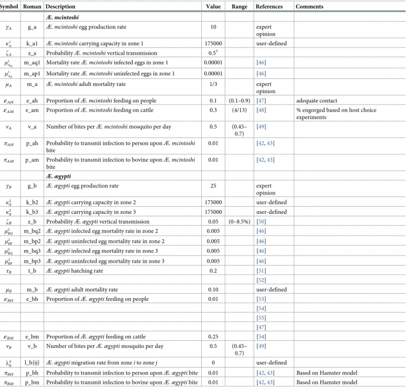
Symbol Roman Description Value References Comments
General
year Number of years (360 days) to run the simulation 27 user-defined
flood_prop proportion flooded annually in floodplain 0.025 user-defined
Oalt O_alt Number of bites by all vector species on alternative hosts 0 user-defined
βwl b _wl Wildlife infection rate 0 user-defined
Human
γH g_h Human birth rate 4/(2�50�360) user-defined
μH m_h Human mortality rate =γH user-defined
ξH x_h Human RVF incubation rate 1/4 (2–6 days) [29]
δH d_h Human RVF-specific mortality rate 1/3�0.01 [29]
αH a_h Human RVF recovery rate 1/3�0.99 [2,29]
ρH r_h Human immunity loss rate 1/900 [41]
lij
H l_h{ij} Human migration rate from zonei to zone j various
†
πHA p_ha Probability to transmit infection from person toÆ. mcintoshi 0.89 (77–100%) [42,43] based on hamster model
πHB p_hb Probability to transmit infection from person toÆ. ægypti 0.89 (77–100%) [42,43] based on hamster model
πHC p_hc Probability to transmit infection from person toCulex sp1 0.81 (78–84%) [42,43] based on hamster model
πHD p_hd Probability to transmit infection from person toCulex sp2 0.81 (78–84%) [42,43] based on hamster model
Zi
H h_h{1, 2, 3} Maximum number of bites per person per day in zonei 25, 25, 25 user-defined
Cattle
gM
U g_m_u Birth rate non-infected cattle 0.00082 user-defined
pAI p_a_i Proportion abortion due to RVF 0.90 user-defined
gM
I g_m_i Birth rate infected cattle ð1 pAIÞ � gMU
ki
M k_m{1, 2, 3} Carrying capacity cattle in zonei 500000 user-defined
μM m_m Cattle mortality rate 0.0008 user-defined
ξM x_m Cattle RVF incubation rate 24/3.25 (12–72 hrs) [44]
[45] based on sheep data
δM d_m Cattle RVF-specific mortality rate 1/3�0.05 OIE disease fact sheet RVF
αM a_m Cattle RVF recovery rate 1/3�0.95 [2]
ρM r_m Bovine immunity loss rate 1/900 [41]
lij
M l_m{ij} Cattle migration rate from zonei to zone j various
‡
φi
MH f_mhi Number of cattle met per person per time unit in zonei 2.5 user-defined
πMA p_ma Probability to transmit infection from bovine toÆ. mcintoshi 0.89 (77–100%) [42,43]
πMB p_mb Probability to transmit infection from bovine toÆ. ægypti 0.89 (77–100%) [42,43]
πMC p_mc Probability to transmit infection from bovine toCulex sp1 0.81 (78–84%) [42,43]
πMD p_md Probability to transmit infection from bovine toCulex sp2 0.81 (78–84%) [42,43]
πMH p_mh00 Probability to transmit infection from bovine to people 0.001 user-defined
ηM h_m Maximum number of bites per bovine per day 50 user-defined
†Currently:
21= 0.005;23= 0.001;12= 0.05;32= 0.05;13= 0.0001;31= 0.005 ‡Currently:
13= 0;23= 0.0001;32= 0.0005;31= 0;21and12seasonal movement from plateau to floodplain
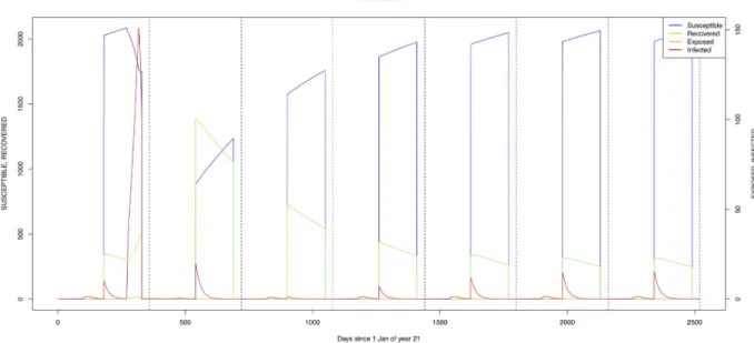
transmission. As shown inFig 15, a vertical transmission rate of 0.25 does not suffice to ensure sufficient numbers of infected eggs to trigger an epidemic at the next El Niño event. No other estimates of this parameter could be traced in the literature and it is recommended that the correct values (ranges) of this important parameter are determined experimentally.
Table 4. Basic model parameters—2.
Symbol Roman Description Value Range References Comments
Æ. mcintoshi
γA g_a Æ. mcintoshi egg production rate 10 expert
opinion k1
A k_a1 Æ. mcintoshi carrying capacity in zone 1 175000 user-defined
zA z_a ProbabilityÆ. mcintoshi vertical transmission 0.5†
m1
AQ m_aq1 Mortality rateÆ. mcintoshi infected eggs in zone 1 0.00001 [46]
m1
AP m_ap1 Mortality rateÆ. mcintoshi uninfected eggs in zone 1 0.00001 [46] μA m_a Æ. mcintoshi adult mortality rate 1/3 expert
opinion
εAH e_ah Proportion ofÆ. mcintoshi feeding on people 0.1 (0.1–0.9) [47] adequate contact
εAM e_am Proportion ofÆ. mcintoshi feeding on cattle 0.3 (4/13) [48] % engorged based on host choice
experiments
νA v_a Number of bites perÆ. mcintoshi mosquito per day 0.5 (0.45–
0.7) [49]
πAH p_ah Probability to transmit infection to person uponÆ. mcintoshi
bite
0.01 [42,43]
πAM p_am Probability to transmit infection to bovine uponÆ. mcintoshi
bite
0.01 [42,43]
Æ. ægypti
γB g_b Æ. ægypti egg production rate 25 expert
opinion k2
B k_b2 Æ. ægypti carrying capacity in zone 2 175000 user-defined
k3
B k_b3 Æ. ægypti carrying capacity in zone 3 175000 user-defined
zB z_b ProbabilityÆ. ægypti vertical transmission 0.05 (0–8.5%) [50]
m2
BQ m_bq2 Æ. ægypti infected egg mortality rate in zone 2 0.005 [46]
m2
BP m_bp2 Æ. ægypti uninfected egg mortality rate in zone 2 0.005 [46] m3
BQ m_bq3 Æ. ægypti infected egg mortality rate in zone 3 0.005 [46]
m3
BP m_bp3 Æ. ægypti uninfected egg mortality rate in zone 3 0.005 [46]
τB t_b Æ. ægypti hatching rate 0.2 [51]
[52]
μB m_b Æ. ægypti adult mortality rate 0.10 user-defined
εBH e_bh Proportion ofÆ. ægypti feeding on people 0.01 [53]
[54] [55] [47]
εBM e_bm Proportion ofÆ. ægypti feeding on cattle 0.25 [54]
νB v_b Number of bites perÆ. ægypti mosquito per day 0.5 (0.45–
0.7) [49] lij
B l_b{ij} Æ. ægypti migration rate from zone i to zone j 0 user-defined
πBH p_bh Probability to transmit infection to person uponÆ. ægypti bite 0.01 [42,43] Based on Hamster model
πBM p_bm Probability to transmit infection to bovine uponÆ. ægypti bite 0.01 [42,43] Based on Hamster model †Values within the published range [0—8.5%, [50]] did not allow infection to be carried by dormant
Æ. mcintoshi eggs from one El Niño event to the next https://doi.org/10.1371/journal.pone.0209929.t004
Table 5. Basic model parameters—3.
Symbol Roman Description Value Range References Comments
Culex sp.1
γC g_c Culex sp1 egg production rate 25 expert opinion
k1
C k_c1 Culex sp1 carrying capacity in zone 1 1750 user-defined
m1
CP m_cp1 Culex sp1 egg mortality rate in zone 1 0.002 user-defined
τC t_c Culex sp1 hatching rate 0.2 user-defined
μC m_c Culex sp1 adult mortality rate 0.10 user-defined
εCH e_ch Proportion ofCulex sp1 feeding on people 0.005 [47] depends on host availability
εCM e_cm Proportion ofCulex sp1 feeding on cattle 0.02 (0–0.9) [47,48] host availability and host choice experiments
νC v_c Number of bites perCulex sp1 mosquito per day 1 user-defined
πCH p_ch Probability to transmit infection to person uponCulex sp1 bite 0.07 (7–37%) [42,43] based on hamster model
πCM p_cm Probability to transmit infection to bovine uponCulex sp1 bite 0.07 (7–37%) [42,43] based on hamster model
Culex sp.2
γD g_d Culex sp2 egg production rate 25 expert opinion
k2
D k_d2 Culex sp2 carrying capacity in zone 2 17500 user-defined
k3
D k_d3 Culex sp2 carrying capacity in zone 3 17500 user-defined
m2
DP m_dp2 Culex sp2 egg mortality rate in zone 2 0.002 user-defined
m3
DP m_dp3 Culex sp2 egg mortality rate in zone 3 0.002 user-defined
τD t_d Culex sp2 hatching rate 0.2 user-defined
μD m_d Culex sp2 adult mortality rate 0.10 user-defined
εDH e_dh Proportion ofCulex sp2 feeding on people 0.005 (0–0.9) [47]
εDM e_dm Proportion ofCulex sp2 feeding on cattle 0.12 (0–0.9) [47,48] host availability and host choice experiments
νD v_d Number of bites perCulex sp2 mosquito per day 1 user-defined
lij
D l_d{ij} Culex sp2 migration rate from zone i to zone j 0 user-defined
πDH p_dh Probability to transmit infection to person uponCulex sp2 bite 0.07 [42,43]
πDM p_dm Probability to transmit infection to bovine uponCulex sp2 bite 0.07 [42,43]
https://doi.org/10.1371/journal.pone.0209929.t005
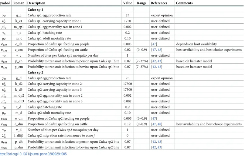
Fig 3. Standard parameters: Human—Zone 1.
A low level of RVFv transmission was predicted by the model (Table 6). Using the standard values, predicted seroprevalence levels in humans and cattle at different times after the El Niño event were comparable to those observed. Seroprevalence is estimated to be 13.2% in people and 12.3% in cattle, six years after an El Niño event. The field studies found similar overall seroprevalence levels of 11.7% in people and 11.3% in cattle, five to six years after the 2006/07 RVF epidemic in the area [17,22]. The results are also in line with previous studies across Africa with evidence of inter-epidemic transmission of RVF [1,15,16]. The dynamics of levels of seroprevalence are of course in the first place dependent on the value employed for the loss-of-serotitre rate: currently a daily value of 1/900 is used, based on a single, rather vague
Fig 5. Standard parameters: Human—Zone 3.
https://doi.org/10.1371/journal.pone.0209929.g005
Fig 4. Standard parameters: Human—Zone 2.
reference [41]. Inclusion of a wildlife reservoir (Table 6, second line) did not have a significant effect on the predicted levels of seroprevalence.
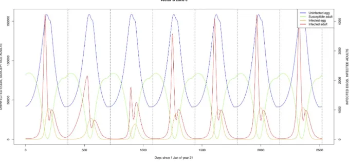
The simulated seroprevalence levels inTable 6in both the human and livestock populations show a gradual decline during the years after an epidemic event (El Niño), which seems to imply low numbers of infective bites during inter-epidemic periods, reflecting the generally low numbers of mosquitoes in the absence of heavy rainfall associated with the El Niño events. People and cattle transiting in the forest (zone 3, Figs5and8) are exposed to infectious bites every year from theÆ. ægypti and Culex sp.2 populations (Figs11and14): the mosquitoes are constantly infected from the wildlife reservoir [56]. People and cattle remaining in the villages
Fig 6. Standard parameters: Cattle—Zone 1.
https://doi.org/10.1371/journal.pone.0209929.g006
Fig 7. Standard parameters: Cattle—Zone 2.
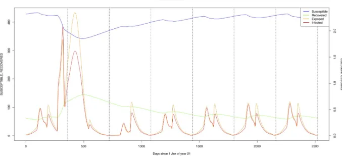
(zone 2, Figs4and7) and/or the floodplains (zone 1, Figs3and6) are minimally exposed on an annual basis with high exposure rates occurring only every ten years (Figs9,10,12and13). Infection thus principally spreads to the villages and floodplains by humans and cattle tempo-rarily residing in the forest zone.
TheÆ. mcintoshi population in the floodplains (Fig 9) is the one maintaining the infection inside the dormant eggs. Adult mosquitoes do not survive the drier period following the El Niño event and only some eggs hatch every year during the partial seasonal flooding of the plain. Substantial hatching occurs during flooding related to the El Niño event in the East Afri-can region, releasing the infection and starting the epidemics. The infection is picked up by
Fig 8. Standard parameters: Cattle—Zone 3.
https://doi.org/10.1371/journal.pone.0209929.g008
Fig 9. Standard parameters:Æ. mcintoshi—Zone 1. https://doi.org/10.1371/journal.pone.0209929.g009
Culex sp.1 present in this area. The human population acquires the infection first, followed by
the cattle population. From there on, the epidemic spreads to the village and the forest with migrating cattle and people.
As indicated by lines three and four ofTable 6(with the current standard parameter set-tings),Æ. mcintoshi on its own is not able to explain the high seroprevalence found in both
humans and cattle [17,22], not even when including annual partial flooding of zone 1 accom-panied by eclosion of part of the dormant eggs. The same can be said forÆ. ægypti, despite it
being resident in the village and forest zones, although it must be understood that in this case the low values for vertical transmission were maintained.
Fig 10. Standard parameters:Æ. ægypti—Zone 2. https://doi.org/10.1371/journal.pone.0209929.g010
Fig 11. Standard parameters:Æ. ægypti—Zone 3. https://doi.org/10.1371/journal.pone.0209929.g011
Lines six to nine ofTable 6examine different scenarios with an efficientCulex vector in the
village and forest zones. Introduction of infection, either by means of a wildlife reservoir (line seven) or through the introduction of an infective animal, allows for maintenance of the infec-tion within the host and vector populainfec-tions. Because of the interacinfec-tion between the different vectors for host-feeding opportunities, the more efficientCulex vector on its own (without
competition fromAedes species) results in higher infection transmission and higher
seropreva-lence levels. Again, a lot more detailed observations are required to properly quantify this aspect of the transmission dynamics.
Mosquito species in the forested environment (Æ. ægypti and Culex sp.2) (Figs11and14) had high annual infection rates. On the other hand, mosquitos in the residential area
Fig 12. Standard parameters:Culex sp.1—Zone 1. https://doi.org/10.1371/journal.pone.0209929.g012
Fig 13. Standard parameters:Culex sp.2—Zone 2. https://doi.org/10.1371/journal.pone.0209929.g013
Fig 14. Standard parameters:Culex sp.2—Zone 3. https://doi.org/10.1371/journal.pone.0209929.g014
Fig 15.Æ. mcintoshi as only vector, no seasonal flooding of zone 1. A: Vertical transmission rate = 0.25; B: Vertical transmission rate = 0.50.
(Æ. ægypti and Culex sp.2) and in the floodplain (Æ. mcintoshi and Culex sp.1) have low
infec-tion rates (Figs9,10,12and13) with peak rates occurring only during or immediately after an El Niño event and subsequent RVF epidemics in the East African region [57].
The model presented here needs further calibrating with datasets from other regions where there are similar or dissimilar ecologies compared to our study area in order to extend and/or improve usability of the model in different geographical, climatic settings. This model, being built with open-source software and with an easy to use interface, can be adapted by research-ers and program managresearch-ers to their specific needs by plugging in new parametresearch-ers relevant to their situation and locality. Its use can be further expanded by including disease prevention and control interventions to model potential impact of these veterinary and public health mea-sures on disease in people and domestic animals, for example vaccination, quarantining and vector control programs.
Supporting information
S1 Appendix. User manual. (PDF)S2 Appendix. Program R code. (PDF)
Author Contributions
Conceptualization: Robert Sumaye, Famke Jansen, Etienne Thiry. Data curation: Robert Sumaye, Famke Jansen.
Table 6. RVF seroprevalence levels (proportion) in people and cattle at different times after an El Niño event.
Human Cattle
EN+2† EN+4 EN+6 EN+2 EN+4 EN+6
Standard 0.209 0.147 0.132 0.324 0.140 0.123 Standard + wl 0.209 0.147 0.132 0.324 0.139 0.122 only Aemc (100A1 Q+ 9900A 1 P)− flood 0.005 0.002 0.001 0.003 0.001 0.000 only Aemc (100A1 Q+ 9900A 1 P) + flood 0.136 0.093 0.078 0.063 0.017 0.006 only Aeae (100B2 Q+ 9900B 2 P) 0.048 0.041 0.039 0.070 0.067 0.067 only Cu2 (1000D3 P) 0.000 0.000 0.000 0.000 0.000 0.000 only Cu2 (1000D3 P) + wl 0.130 0.138 0.141 0.034 0.035 0.035 only Cu2 (1000D2 P) 0.000 0.000 0.000 0.000 0.000 0.000 only Cu2 (1000D2 P) + introduction of 1M 2 I 0.177 0.186 0.189 0.132 0.136 0.136 †
EN+2/4/6 = year 2/4/6 after El Niño event • Standard: 1000H2 S, 2500M 2 S, 100A 1 Q, 9900A 1 P, 10B 3 P, 100C 1 P, 1000D 2 S, 1000D 3 P
• Standard + wl: as above + wildlife reservoir (infection rate for vectors = 1e-5) • only Aemc (100A1
Q+ 9900A 1
P)− flood: Æ. mcintoshi 100 infected eggs, 9900 uninfected eggs in zone 1, no annual partial flooding of zone 1
• only Aemc (100A1 Q+ 9900A
1
P) + flooding: as above + annual partial flooding of zone 1
• only Aeae (100B2 Q+ 9900B
2
P):Æ. ægypti 100 infected eggs, 9900 uninfected eggs in zone 2
• only Cu2 (1000D3
P):Culex sp.2 1000 eggs in zone 3
• only Cu2 (1000D3
P): as above + wildlife reservoir (infection rate for vectors = 1e -5
) • only Cu2 (1000D2
P):Culex sp.2 1000 eggs in zone 2
• only Cu2 (1000D2
P) + introduction of 1M 2
I: as above with introduction of one infective bovine in Zone 2
Formal analysis: Meryam Krit.
Investigation: Robert Sumaye, Famke Jansen. Methodology: Dirk Berkvens, Bernard De Baets.
Project administration: Dirk Berkvens, Eveline Geubels, Etienne Thiry. Resources: Robert Sumaye, Eveline Geubels.
Software: Meryam Krit.
Supervision: Dirk Berkvens, Meryam Krit. Validation: Bernard De Baets.
Writing – original draft: Robert Sumaye, Famke Jansen. Writing – review & editing: Dirk Berkvens, Meryam Krit.
References
1. Evans A, Gakuya F, Paweska JT, Rostal M, Akoolo L, Van Vuren PJ, et al. Prevalence of antibodies against Rift Valley fever virus in Kenyan wildlife. Epidemiol Infect. 2008; 136(9):1261–1269.https://doi.
org/10.1017/S0950268807009806PMID:17988425
2. Swanepoel R, Coetzer JAW. Rift Valley fever. In: Coetzer JAW, Tustin RC, editors. Infectious diseases of livestock in Southern Africa. vol. 2. Oxford University Press; 2004. p. 1037–1059.
3. Daubney R, Hudson JR. Enzootic hepatitis or Rift Valley fever. Journal of Pathology. 1931; 34:545– 579.https://doi.org/10.1002/path.1700340418
4. Davies FG. The Historical and Recent Impact of Rift Valley Fever in Africa. American J Trop Med Hyg. 2010; 83:73–74.https://doi.org/10.4269/ajtmh.2010.83s2a02
5. Di Nardo A, Rossi D, Saleh SML, Lejifa SM, Hamdi SJ, Di Gennaro A, et al. Evidence of risft valley fever seroprevalence in the Sahrawi semi-nomadic pastoralist system, Western Sahara. BMC Vet Res. 2014; 10:92.https://doi.org/10.1186/1746-6148-10-92PMID:24758592
6. Bosworth A, Ghabbari T, Dowall S, Varghese A, Fares W, Hewson R, et al. Serological evidence of exposure to Rift Valley fever virus detected in Tunisia. New Microbes and New Infect. 2016; 9:1–7.
https://doi.org/10.1016/j.nmni.2015.10.010
7. Failloux AB, Bouattour A, Faraj C, Gunay F, Haddad N, Harrat Z, et al. Surveillance of Arthropod-Borne Viruses and Their Vectors in the Mediterranean and Black Sea Regions Within the MediLabSecure Net-work. Curr Trop Med Rep. 2017; 4(1):27–39.https://doi.org/10.1007/s40475-017-0101-yPMID:
28386524
8. Gu¨r S, Kale M, Erol N, Yapici O, Mamak N. The first serological evidence for Rift Valley fever infection in camel, goitered gazelle and Anatolian water buffaloes in Turkey. Trop Anim Health and Prod. 2017; 49 (7):1531–1535.https://doi.org/10.1007/s11250-017-1359-8
9. WHO. Rift Valley fever in China; 2016. Available from: http://www.who.int/csr/don/02-august-2016-rift-valley-fever-china/en/[cited 2017/07/12].
10. Anyamba A, Chretien JP, Small J, Tucker CJ, Formenty PB, Richardson JH, et al. Prediction of a Rift Valley fever outbreak. Proceedings of the National Academy of Sciences of the United States of Amer-ica. 2009; 106:955–959.https://doi.org/10.1073/pnas.0806490106PMID:19144928
11. Davies FG, Linthicum KJ, James AD. Rainfall and epizootic Rift Valley fever. Bull World Health Organ. 1985; 63:941–943. PMID:3879206
12. Chevalier V, Thiongane Y, Lancelot R. Endemic transmission of Rift Valley fever in Senegal. Trans-bound Emerg Dis. 2009; 56(9-10):372–374.https://doi.org/10.1111/j.1865-1682.2009.01083.xPMID:
19548898
13. Wilson ML, Chapman LE, Hall DB, Dykstra EA, Ba K, Zeller HG, et al. Rift Valley fever in rural Northern Senegal: human risk factors and potential vectors. Am J Trop Med Hyg. 1994; 50:663–675.https://doi. org/10.4269/ajtmh.1994.50.663PMID:7912905
14. Durand JP, Bouloy M, Richecoeur L, Peyrefitte CN, Tolou H. Rift Valley fever virus infection among French troops in Chad. Emerg Infect Dis. 2003; 9(6):751–752.https://doi.org/10.3201/eid0906.020647
15. LaBeaud AD, Muchiri EM, Ndzovu M, Mwanje MT, Muiruri S, Peters CJ, et al. Interepidemic Rift Valley fever virus seropositivity, northeastern Kenya. Emerg Infect Dis. 2008; 14(8):1240–1246.https://doi. org/10.3201/eid1408.080082PMID:18680647
16. LaBeaud AD, Cross PC, Getz WM, Glinka A, King CH. Rift Valley fever virus infection in African buffalo (Syncerus caffer) herds in rural South Arica: evidence of interepidemic transmission. Am J Trop Med Hyg. 2011; 84(4):641–646.https://doi.org/10.4269/ajtmh.2011.10-0187PMID:21460024
17. Sumaye RD, Geubbels E, Mbeyela E, Berkvens D. Inter-epidemic transmission of Rift Valley fever in livestock in the Kilombero River Valley, Tanzania: a cross-sectional survey. PLoS Negl Trop Dis. 2013; 7(8):e2356.https://doi.org/10.1371/journal.pntd.0002356PMID:23951376
18. Swai ES, Schoonman L. Prevalence of Rift Valley fever immunoglobulin G antibody in various occupa-tional groups before the 2007 outbreak in Tanzania. Vector-borne and Zoonotic Dis. 2009; 9(6):579– 582.https://doi.org/10.1089/vbz.2008.0108
19. Mohamed M, Mosha F, Mghamba J, Zaki SR, Shieh WJ, Paweska J, et al. Epidemiologic and clinical aspects of a Rift Valley fever outbreak in humans in Tanzania, 2007. Am J Trop Med Hyg. 2010; 83(2 Suppl):22–27.https://doi.org/10.4269/ajtmh.2010.09-0318PMID:20682902
20. Woods CW, Karpati AM, Grein T, McCarthy N, Gaturuku P, Muchiri E, et al. An outbreak of Rift Valley fever in Northeastern Kenya, 1997-98. Emerg Infect Dis. 2002; 8(2):138–144. PMID:11897064
21. WHO. Outbreaks of Rift Valley fever in Kenya, Somalia and United Republic of Tanzania, December 2006—April 2007. Weekly Epidemiological Record. 2007; 82:169–178. PMID:17508438
22. Sumaye RD, Abatih EN, Thiry E, Amuri M, Berkvens D, Geubbels E. Inter-epidemic acquisition of Rift Valley fever virus in humans in Tanzania. PLoS Negl Trop Dis. 2015; 9:e0003536.https://doi.org/10. 1371/journal.pntd.0003536PMID:25723502
23. Anderson EC, Rowe LW. The prevalence of antibody to the viruses of bovine virus diarrhoea, bovine herpes virus 1, rift valley fever, ephemeral fever and bluetongue and to Leptospira sp in free-ranging wildlife in Zimbabwe. Epidemiol Infect. 1998; 121:441–449.https://doi.org/10.1017/
S0950268898001289PMID:9825798
24. Abu Elyazeed R, El-Sharkawy S, Olson J, Botros B, Soliman A, Salib A, et al. Prevalence of anti-Rift-Valley-fever IgM antibody in abattoir workers in the Nile delta during the 1993 outbreak in Egypt. Bull World Health Organ. 1996; 74:155–158. PMID:8706230
25. Archer BN, Weyer J, Paweska J, Nkosi D, Leman P, Tint KS, et al. Outbreak of Rift Valley Fever affect-ing veterinarians and farmers in South Africa, 2008. S Afr Med J. 2011; 101:263–266.https://doi.org/10.
7196/SAMJ.4544PMID:21786732
26. McIntosh BM, Russell D, Dos Santos I, Gear JHS. Rift Valley Fever in humans in South Africa. S Afr Med J. 1980; 58(20):803–806. PMID:7192434
27. Kitchen SF. Laboratory infections with the virus of Rift Valley fever. Am J Trop Med Hyg. 1934; 1:547– 564.https://doi.org/10.4269/ajtmh.1934.s1-14.547
28. Smithburn KC, Mahaffy AF, Haddow AJ, Kitchen SF, Smith JF. Rift Valley fever: accidental infections among laboratory workers. J Immunol. 1949; 62(2):213–227. PMID:18153372
29. WHO. Rift Valley fever fact sheet. Weekly Epidemiological Record. 2008; 83:17–24. PMID:18188879
30. Anyangu AS, Gould LH, Sharif SK, Nguku PM, Omolo JO, Mutonga D, et al. Risk factors for severe Rift Valley fever infection in Kenya, 2007. The Am J Trop Med and Hyg. 2010; 83:14–21.https://doi.org/10. 4269/ajtmh.2010.09-0293
31. Madani TA, Al-Mazrou YY, Al-Jeffri MH, Mishkas AA, Al-Rabeah AM, Turkistani AM, et al. Rift Valley fever epidemic in Saudi Arabia: epidemiological, clinical and laboratory characteristics. Clin Infect Dis. 2003; 37(8):1084–1092.https://doi.org/10.1086/378747PMID:14523773
32. Rich KM, Wanyoike F. An assessment of the regional and national socio-economic impacts of the 2007 Rift Valley fever outbreak in Kenya. Am J Trop Med Hyg. 2010; 83(2 Suppl):52–57.https://doi.org/10. 4269/ajtmh.2010.09-0291PMID:20682906
33. Al-Hazmi M, Ayoola EA, Abdurahman M, Banzal S, Ashraf J, El-Bushra A, et al. Epidemic Rift Valley fever in Saudi Arabia: a clinical study of severe illness in humans. Clin Infect Dis. 2003; 36:245–252.
https://doi.org/10.1086/345671PMID:12539063
34. Soti V, Chevalier V, Maura J, Be´gue´ A, Lelong C, Lancelot R, et al. Identifying landscape features asso-ciated with Rift Valley fever virus transmission, Ferlo region, Senegal, using very high spatial resolution satellite imagery. Int J Health Geogr. 2013; 12:1–11.https://doi.org/10.1186/1476-072X-12-10
35. Arsevska E, Hellal J, Mejri S, Hammami S, Marianneau P, Calavas D, et al. Identifying Areas Suitable for the Occurrence of Rift Valley Fever in North Africa: Implications for Surveillance. Transbound Emerg Dis. 2016; 63:658–674.https://doi.org/10.1111/tbed.12331PMID:25655790
36. Gaff HD, Hartley DM, Leahy NP. An Epidemiological Model of Rift Valley Fever. Electronic Journal of Differential Equations. 2007; 115:1–12.