DECENTRALIZED MECHANICAL VENTILATION
WITH HEAT RECOVERY
Cleide Aparecida Silva 1, Samuel Gendebien 2, Jules Hannay 1, Nicolas Hansens 3, Jean Lebrun 1*, Marc Lengele 4, Gabrielle Masy s 3, Luc Prieels 5
1 JCJ Energetics Liège, Belgium [email protected] 2 Thermodynamics Laboratory University of Liège Liège, Belgium 4 WOW Technology Nannine, Belgium 3 CECOTEPE Liège, Belgium 5 Greencom Development SCRL Liège, Belgium ABSTRACT
A new local ventilation device is designed in such a way to procure ventilation “on demand” in each room, with a maximum of effectiveness and a minimum of energy waste.
It consists in a parapipedic box to be located in one external wall (for example, just above a window) and containing two (injection and extraction) fans and a recovery heat exchanger. The design of the heat exchanger is associated to the selection of the two fans in view of the best compromise between heat recovery effectiveness and “auxiliary” consumptions. Great attention is paid to supply and exhaust air openings on both indoor and outdoor sides of the device, in order to get the highest ventilation effectiveness.
A fair compromise is looked for between air flow control “authority” and “auxiliary” consumption.
KEYWORDS
Ventilation, air diffusion, heat recovery, control, simulation
1. INTRODUCTION
Indoor climate control means satisfying some requirements on the following items, in order of decreasing priorities:
- Air quality
- Environmental temperature - Air moisture
Developing more and more efficient ventilation techniques is a key issue, in the design of new “low” (and “zero”) energy buildings, as well as in the retrofit of existing ones. Such development should include the following considerations: 1) Making ventilation “on demand” in such a way to maintain the required air quality in each occupied building zone; 2) Maximizing the ventilation effectiveness, i.e. keeping the required air quality inside the occupancy zones with as little air renovation as possible; 3) Minimizing the global energy consumption of the ventilation system;
4) Paying attention to all possible “side effects”, as risk of draught effect, noise, sound transmission (and privacy loss)…
These considerations are hereafter further developed, as a continuation of a previous presentation [1].
2. STEP BY STEP DESIGN OF A VENTILATION SYSTEM: BACK TO THE BASIC PRINCIPLES
The following steps can be distinguished:
2.1. Identify the contaminants and the tolerable concentrations
2.2. Capture the contaminants as near as possible to the contamination sources, before they may be dispersed in the air of the occupancy (or breathing) zone, thanks to velocity control and local extraction. This is feasible if the contamination source is fixed, as, for example, in an industrial process or above a cooking appliance, but not if the contamination is issued from occupants, moving inside the room.
2.3. Bring fresh air as directly as possible into the breathing zone, thanks to velocity control and local supply. This is feasible if the occupant to be protected has fixed position inside the room (as, for example, in an office, in a theatre, or in a surgery room).
Both actions 2.2 and 2.3 can be (partially) realized with or without mechanical system. One or the two actions might be sufficient, but both can also be partially combined, in so-called “displacement” ventilation. But caution has to be paid to some side effects, as, for example, the risk of draught…
2.4. Having a fair idea of achievable ventilation effectiveness, identify the best combination of air regeneration (with contaminants capture by filtering and other separation methods) and air renewal. On earth (but not in a space vehicle!) the re-introduction of O2 (and elimination of CO2) is usually performed by air renewal and CO2 is the current tracer, taken as reference to determine the required fresh air flow rate.
Fresh air can be supplied to the occupants by “passive”, “active”, or “hybrid” methods. The choice among these possibilities should result from a careful analysis of building
tightness (including all fixed and variable openings), indoor and outdoor climates (buoyancy and wind effects) and resulting “natural” infiltrations.
2.5. Decide which part of the fresh air flow rate (if any) has to be provided by “active” means, i.e. by mechanical ventilation, with careful considerations to main advantages, inconveniences and side effects. Modify some of the building characteristics, if desirable and feasible; for example, improve its tightness and/or take control of some of the variable openings. Free heating and free cooling are examples of advantages and inconveniences to be
considered, according to the season. Noise generation, noise transmission and draughts are again among side effects to be taken in consideration.
2.6. Decide how to organize the mechanical ventilation, with central and/or local supply and exhaust systems.
2.7. Decide how to control the ventilation system, in such a way to get the correct air quality in each zone, with minimal fresh air flow rate.
Control design requires identifying the “controllability” of the whole (building and
mechanical ventilation) system considered, which includes: - The controllability of the mechanical ventilation itself, which can be defined as the ratio between ventilator head and total head (fan + wind + buoyancy);
- The mechanical ventilation “authority”, i.e. the pressure range in which mechanical ventilation is able to “impose” any (minimal or maximal) air flow rate. The ventilation authority is satisfactory if this pressure range is larger than all combined wind and buoyancy perturbations.
- The controllability of the whole (building and mechanical ventilation) system is fully satisfactory if the total (mechanical and natural) fresh air flow rate can be controlled in each building zone and if all zone-to-zone air circulations are also under control. This last
requirement can be very important, for example if having to deal with the risk of odour propagation from one zone to another one. It may justify some supply/exhaust disequilibrium inside a same zone (supplying more fresh air to “clean” zones and extracting more from “dirty” ones).
2.8. Minimize the (energy and/or environmental) impacts of the ventilation, thanks to heat recovery.
3. THE SYSTEM UNDER DEVELOPMENT
The new local ventilation system still under development is designed in such a way to procure ventilation “on demand” in each room, with a maximum of effectiveness and a minimum of energy waste.
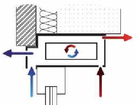
It consists in a parapipedic box to be located in one external wall (for example, just above a window as shown in Figure 1) and containing two (injection and extraction) fans and a recovery heat exchanger [1], [2], [3].
Figure 1. Typical configuration of the local ventilation system
The first applications considered are in the residential buildings, but other buildings, as offices, schools and health services are also concerned.
3.1. Air diffusion analyses
3.1.1. Air diffusion inside the ventilated enclosure can be described by the model presented in Figure 2. Dominant air movements are here supposed to be induced by the following sources
[1]: - Ventilation and infiltration jets
- Buoyancy jet(s) issued from radiator(s) - Buoyancy jet(s) issued from the occupant(s)
- Free convection boundary layers along cold walls (mainly the windows).
Three horizontal zones are distinguished in the model, as suggested in Figure 2, where the left and right sides are only distinguished for readability (the radiator is usually not located in opposition to the frontage).
In principle, fresh air can be supplied and exhausted to and from one, two or three different zones. But, in the case considered supply and exhaust openings are only located in zone 3. If there is no phase change inside the room, the distribution of the air moisture can be considered as similar to the distribution of the contaminant.
The model consists in two sets of equations describing the induction effects and the balances of air, contaminant, sensible heat and moisture.
For example, the air mass balance of the first zone is described by the following equation:
The different terms correspond to the air supply to this zone, the flow rate from zone 2 to zone 1 induced by the supply air jet of zone 1, the flow rate from zone to zone 2 induced by the supply air jet of zone 2, the flow rate “aspirated” by the radiator(s), the (positive or negative) displacement flow from zone 2 to zone 1, the flow rate supplied to zone one by free convection along the cold wall(s) and the air flow rate extracted from the zone.
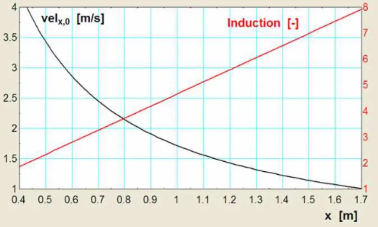
3.1.2. Avoiding local short-circuits on both indoor and outdoor sides requires, not only requires a careful design of the shapes of both openings, but also a sufficiently high velocity at box exhaust, in such a way to avoid that the exhaust jet would be deviated toward the aspiration opening by wind (on outdoor side) and/or buoyancy effects (on both sides). Rain water capture has also to be avoided at outdoor fresh air aspiration.
On both side of the system, there is a need of ensuring enough air mixing before getting any risk of jet deflexion. An example of verification is shown in Figure 3: it corresponds to the rejection of 60 m3/h of air, at 4 m/s of initial speed, through a circular opening. In this case, an induction factor of the order of 8 is already reached, when the jet axial velocity is reduced to 1 m/s (considered as a still sufficient “control” velocity). This means that the risk of short circuit is very reduced…
Figure 3. Diffusion of a jet issued from a circular orifice 3.1.3 Avoiding local discomfort
Inside the room, there is a risk of draught discomfort, if the jet is not diluted enough before entering the occupation zone.
The deviation due to buyancy can be verified by simulation as shown in Figure 4. In this example the air is supplied trough a rectangular opening at the rate of 35 m3/h and at a temperature of 10 C, with an idoor air temperature of 20 C. Three different initial speeds are considered: 1, 2 and 3 m/s. In this case, the initial speed must be maintained above 2 m/s, in order to avoid any risk of discomfort.
Of course, such simulation models have all to be tuned by experiments. A series of tests is also being performed in a climatic room…
3.2. Air diffusion effectiveness
In order of decreasing importance, air diffusion effectiveness can be defined according to its effects on air quality, environmental temperature and air moisture.
Each effectiveness results of the combination of two phenomena:
- The “displacement” (also called “plug flow”), whose effect is a fictitious reduction of contamination flow rate;
- The mixing, whose effect is to eliminate any risk of short circuit, which would itself produce a fictitious reduction of air renewal
Displacement and mixing effectiveness’s can be defined by the following equations:
(Considering three sources of contamination: the occupants, the materials and the terminal units).
Similar equations can be used for sensible heat and moisture (with the same sources as for the contamination, plus the sun for sensible heat)…
In the case considered here, it seems that the air diffusion effectiveness is, most of the time, near to 1, but this has also has still to be experimentally verified…
3.3. Control
A high authority is provided by the system considered [2] [3], as shown in Figure 5: each variable speed fan is selected as able to keep the required air flow rate in a broad domain of pressure drop: from +110 to – 30 Pa. Above 110 Pa, the fan stays at its maximal speed; below -30 Pa, the fan is stopped.
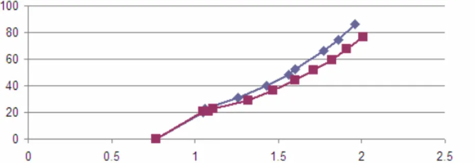
A feed back control of the air flow rate is performed on the basis of a signal given by a thermal anemometer located inside each ventilation channel. Each probe is calibrated is such a way to get a reliable correlation between air speed and corresponding flow rate, as shown in Figure 6.
Figure 6: Example of correlation between flow rate (y) and air speed (x)
3.5 Recovery
Three « local » recovery effectiveness’s can be defined at the level of the mechanical ventilation system:
A « good » ventilation system is usually characterized by a very low value of the first effectiveness and high values of the two other ones [1] [4].
But this is not the whole of it: a global energy balances need to be establiched, by
considering, not only the heat recovery, but also the “auxiliary” consumption of the system. Examples of heat exchanger tests results are presented in Figure 7. At reference flow rate of 36 m3/h, the pressure drop of this heat exchanger is of the order of 60 Pa and its thermal effectiveness might over-pass 85 %.
But these results were obtained on the heat exchanger alone, i.e. not yet installed in the box. Some extra-pressure drops and losses of effectiveness have to be taken into account because of the non-uniform distribution of supply air at both sides of the heat exchanger.
Figure 7. Example of heat exchanger test results [4]: pressure drop in Pa and thermal effectiveness in %.
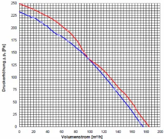
The centrifugal fans selected for this system are over-sized in order to reduce their noise. Examples of fans characteristics, at nominal rotation speed, are shown in Figures 8 and 9.
Figure 8: Pressure-flow characteristic of the fan
Figure 9: Electrical power consumed by the fan
Thanks to the over-sizing, the fans can be runned at low rotation speed (and low noise generation). Acoustic tests are also being made on the fans and on the whole system. Not only the two fans, but also the control unit is consuming energy.
At nominal flow rate of 36 m3/h the electrical consumption the smallest unit considered should not over-pass 5 W.
If runned continuously on a full reference year of 2000 degree-days, such unit should be able to recover about 480 kWh of sensible heat and would not consume more than about 45 kWh. This would give an average COP higher than 10.
And this COP can be significantly increased if the unit is stopped whenever the heat recovery is too small, i.e. in mid season and summertime, when natural ventilation might be preferred.
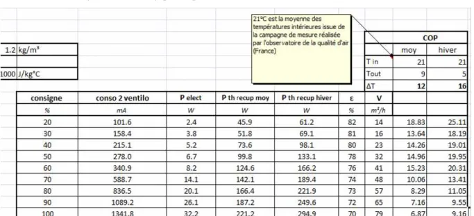
Examples of more detailed results are presented in tables 1 and 2 and in Figure 10. In table 1 are presented the average performances (one the whole year and on the winter season) as functions of the fans rotation speeds, with the following nomenclature:
“consigne”: ratio between actual and nominal fan speed [%]
Conso2ventilo: electrical current consumed by both fans [mA] (under 24 V DC) Pelect: electrical power [W]
Pth recup moy: mean thermal power recovered on the whole year [W] Pth recup hiver: mean thermal power recovered on winter time [W] Epsilon: thermal effectiveness [%]
V: air flow rates (on both sides) [m3/h]
Table 1: Average performances calculated for different fans rotation speeds The same results are presented month by month in table 2 and in Figure 10, with:
P(x)th rec= mean thermal power recovered with both fans at x % of their nominal speed. These very encouraging results might be a bit optimistic because they are still based on separate tests of the different components and also because they don’t consider the actual building energy balance which would make useless a part of the recovery…
Figure 10: Monthly COP’s for three different rotation speeds
“Passive” and “active” recovery techniques were also previously compared according to their respective impacts on the energy demand on a typical dwelling [1].
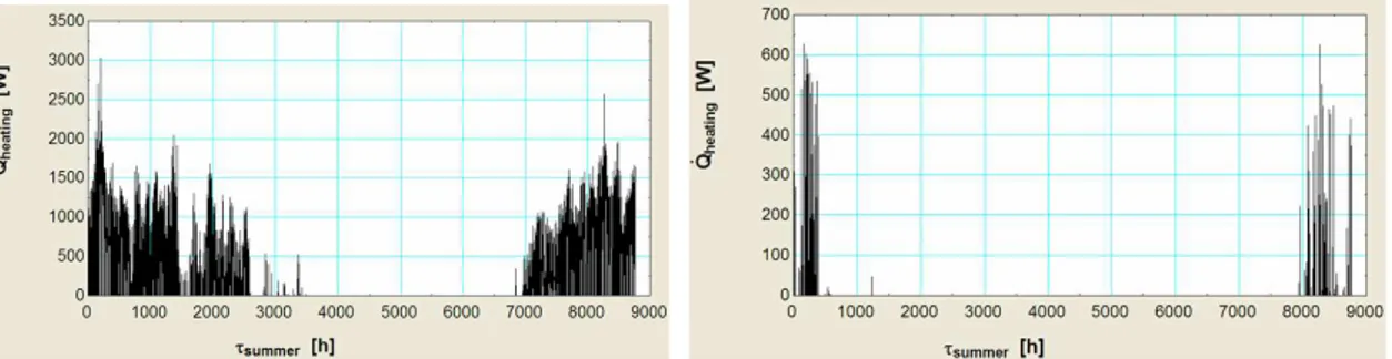
Examples of results are presented in Figure 10:
The dwelling is equipped with a mechanical ventilation system, without any heat recovery. The living room is supplied with 75 m3/h and two of the three sleeping rooms with 30 m3/h of fresh air. Only one sleeping room is occupied and all the surrounding dwellings are fully occupied. The space heating demand without any recovery is plotted on left side of Figure 9. It corresponds to 2667 kWh per year.
A (very) small heat pump is then supposed to be added inside each local ventilation system. This heat pump is acting downstream of the heat exchanger: it under-cools the exhaust air and over-heats the fresh air. The fresh air supply temperature is supposed to be raised until a maximum of 40°C.
The global contribution of these three small heat pumps is very significant, as shown on the right side of Figure 10: the remaining space heating demand to be covered by another heating source is marginal: it doesn’t overpass 600 W and corresponds to only 65 kWh per year. But such very small heat pumps are not yet available on the market and such solution will probably not be cost effective in near future…
CONCLUSIONS
The local ventilation system appears as a very promising solution. It should allow an effective control the indoor air quality, with satisfactory thermal comfort and significant energy savings.
But many experimental verifications are still necessary, mainly about the correct air diffusion inside the room. This is so whenever dealing with a new terminal unit: simulation models need always to be tuned.
The system considered is of particular interest when having to deal with a very variable building occupancy…
ACKNOWLEDGEMENTS
The support of the Walloon Region for funding the Green+ project in the framework of the “Marshall Plan” to the work related in this project is gratefully acknowledged.
REFERENCES
[1] Aparecida Silva Cl., Hannay J., Lebrun J., Prieels L. Development of an ew ventilation system with heat recovery Roomvent 2011
[2] Lebrun J., Prieels L., Vincent B., Hansen N. A model of decentralized air handling terminals (DAHT) interacting with building infiltration Roomvent 2011 [3] Masy G., Lebrun J., Gendebien S., Hansen N., Lengele M., Prieels L. Performances of DAHT conntected to building airtightness and indoor air hygrothermal climate
AIVC TIGHTVENT Conference 2011
[4] Samuel Roomvent Gendebien S., Bertagnolio St., Georges B., Lemort V. Investigation on an air-to-air heat recovery exchanger: modeling and experimental validation Roomvent 2011