HAL Id: hal-01905701
https://hal.sorbonne-universite.fr/hal-01905701
Submitted on 26 Oct 2018
HAL is a multi-disciplinary open access
archive for the deposit and dissemination of
sci-entific research documents, whether they are
pub-lished or not. The documents may come from
teaching and research institutions in France or
abroad, or from public or private research centers.
L’archive ouverte pluridisciplinaire HAL, est
destinée au dépôt et à la diffusion de documents
scientifiques de niveau recherche, publiés ou non,
émanant des établissements d’enseignement et de
recherche français ou étrangers, des laboratoires
publics ou privés.
The cumulative impacts of small reservoirs on
hydrology: A review
Florence Habets, Jérôme Molenat, Nadia Carluer, Olivier Douez, Delphine
Leenhardt
To cite this version:
Florence Habets, Jérôme Molenat, Nadia Carluer, Olivier Douez, Delphine Leenhardt. The cumulative
impacts of small reservoirs on hydrology: A review. Science of the Total Environment, Elsevier, 2018,
643, pp.850-867. �10.1016/j.scitotenv.2018.06.188�. �hal-01905701�
The cumulative impacts of small reservoirs on hydrology: a review
Highlights
• The number of small dams is still increasing and is approaching 39 dams per square kilo-metre
• Small dams lead to a decrease in annual stream discharge of 13% ± 8% • Cumulative impacts cannot be estimated using simple indicators
• Cumulative impacts are difficult to estimate and are most often quantified from modelling • The lack of information on small reservoir characteristics is a real shortcoming for properly
estimating their cumulative impacts
Email addresses: florence.habets@upmc.fr (Habets Florence ), jerome.molenat@inra.fr (Mol´enat J´erˆome )
The cumulative impacts of small reservoirs on hydrology: a review
Habets Florencea,∗, Mol´enat J´erˆomeb,∗, Carluer Nadiac, Douez Olivierd, Leenhardt DelphineeaCNRS/Sorbonne Universit´e, UMR 7619 Metis, Paris, France
bUMR LISAH, Univ Montpellier, INRA, IRD, Montpellier SupAgro, Montpellier, France cIrstea, UR RiverLy, centre de Lyon-Villeurbanne, 69625 Villeurbanne, France
dBRGM, Bordeaux, France
eToulouse Univ, INRA, INPT, INP EI PURPAN, AGIR, Castanet Tolosan, France
Abstract
The number of small reservoirs has increased due to their reduced cost, the availability of many favourable locations, and their easy access due to proximity. The cumulative impacts of such small reservoirs are not easy to estimate, even when solely considering hydrology, which is partially due to the difficulty in collecting data on the functioning of such reservoirs. However, there is evidence indicating that the cumulative impacts of such reservoirs are significant.
The aim of this article is to present a review of the studies that address the cumulative impacts of small reservoirs on hydrology, focusing on the methodology and on the way in which these impacts are assessed.
Most of the studies addressing the hydrological cumulative impacts focused on the annual stream discharge, with decreases ranging from 0.2% to 36% with a mean value of 13.4% ±8% over approximately 30 references. However, it is shown that similar densities of small reservoirs can lead to different impacts on stream discharge in different regions. This result is probably due to the hydro-climatic conditions and makes defining simple indicators to provide a first guess of the cumulative impacts difficult. The impacts also vary in time, with a more intense reduction in the river discharge during the dry years than during the wet years. This finding is certainly an important point to take into consideration in the context of climate change.
Two methods are mostly used to estimate cumulative impacts: i) exclusively data-based methods and ii) models. The assumptions, interests and shortcomings of these methods are presented. Scientific tracks are proposed to address the four main shortcomings, namely the es-timation of the associated uncertainties, the lack of knowledge on reservoir characteristics and water abstraction and the accuracy of the impact indicators.
1. Introduction
1
Large reservoirs have strong impacts on hydrology at regional to global scales. Indeed, it
2
was estimated that such large reservoirs have led to a global runoff decrease of approximately
3
2% (Biemans et al., 2011), to a sea level decrease of approximately 30 mm (Chao et al., 2008),
4
and that they store a volume equivalent to approximately 10% of the natural annual soil storage
5
capacity at the global scale (Zhou et al., 2016). However, these studies did not consider the
6
impacts of smaller reservoirs on hydrology. Downing (2010) found that small ponds and lakes
7
(smaller than 0.1km2) cover a larger area and are more numerous than large reservoirs and that
8
approximately 10% of them are constructed reservoirs.
9
When considered individually, each reservoir may modify its local and remote environment.
10
The cumulative impacts of many reservoirs in a catchment are the modifications induced by a set
11
of reservoirs (or reservoir network) taken as a whole. The cumulative impacts are not necessarily
12
the sum of individual modifications because reservoirs may be inter-dependent, such as cascading
13
reservoirs along a stream course. Cumulative impacts are not the simple addition of individual
14
impacts: they can develop via an additive or incremental process, a supra-additive process (where
15
the cumulative effect is greater than the sum of the individual effects) or an infra-additive process
16
(where the cumulative effect is less than the sum of the individual effects). The total impact is
17
therefore equal to the sum of the impacts of the developments and to interaction effects. Indeed,
18
addressing the cumulative impacts implies covering different spatial and temporal scales (Canter
19
and Kamath, 1995) and having a reference state (McCold and Saulsbury, 1996). The cumulative
20
impacts of small reservoirs on sediment transport, biochemistry, ecology and greenhouse gas
21
emissions have been studied (Berg et al., 2016; Mbaka and Wanjiru Mwaniki, 2015; Downing,
22
2010; Poff and Zimmerman, 2010; St. Louis et al., 2000), as have the impacts of such reservoirs
23
on hydrology (Nathan and Lowe, 2012; Fowler et al., 2015). The reported impacts are generally
24
strong but present a large variation.
25
Estimating the cumulative impacts of systems of small reservoirs on a given basin has become
26
an issue as their number increases (for instance, a 3% increase per year in the US (Berg et al.,
27
2016)). This trend may persist because these systems are often considered to be a technique to
28
∗The authors contributed equally
Email addresses: florence.habets@upmc.fr (Habets Florence ), jerome.molenat@inra.fr (Mol´enat J´erˆome )
adapt to climate change (van der Zaag and Gupta, 2008). Indeed, small reservoirs are mainly
29
used to store water during the wet season to support water use during the dry season, particularly
30
for irrigation and livestock in rural areas (Wisser et al., 2010; Nathan and Lowe, 2012); to store
31
water during storms to prevent flooding; or to store sediments in check dams to reduce erosion
32
and muddy flood risks. Because the part of the global population that will experience water
33
scarcity is projected to increase with climate change and because the intensity of storm events is
34
also projected to simultaneously increase (Pachauri et al., 2014), there is increasing pressure to
35
construct small reservoirs (van der Zaag and Gupta, 2008; Thomas et al., 2011).
36
However, an uncontrolled development of such small reservoirs may increase the water
re-37
source problem in both quantitative and qualitative ways. Thus, water managers are seeking some
38
indicators that would help to determine optimal networks of small reservoirs in terms of storage
39
capacities and in terms of locations and management. Consequently, in France, the Ministry of
40
the Environment requested a joint scientific assessment to collect useful information/knowledge
41
and tools to provide local stakeholders with such indicators and methods to assess the cumulative
42
impacts of small reservoirs. This request led to a review covering biochemistry, ecology,
hydrol-43
ogy and hydromorphology (Carluer et al., 2016). In this paper, a full review of the cumulative
44
impacts of small reservoirs on hydrology is presented because the hydrological impact will affect
45
the other impacts. Although there is no accepted definition of small reservoirs, it is commonly
46
accepted that the storage capacities of such reservoirs are below 1 million m3, as stated by Ayalew
47
et al. (2017) and Thomas et al. (2011). This review does not extend to the very small reservoirs
48
of few hundreds of m3that can be used for water harvesting (Lasage and Verburg, 2015).
49
First, a synthesis of the quantification of the impacts at the basin scale is presented, and the
50
ability of some conventional descriptors to be used as indicators is studied. Then, the various
51
ways in which small reservoirs can impact the water cycle are presented, along with the methods
52
that are used in the literature to estimate the cumulative impacts of such numerous and not always
53
well-known structures. These results are then discussed, addressing the uncertainties, long-term
54
trends, and impacts on other biochemical, ecological and social components.
55
2. Evidence of the impacts of small reservoirs on hydrology
56
From the literature review, the cumulative impacts of small reservoirs on hydrology are most
57
often estimated from the annual discharge, low flows and floods. There is a general consensus
that sets of small reservoirs lead to a reduction in the flood peaks (Frickel, 1972; Galea et al.,
59
2005; Nathan and Lowe, 2012; Thompson, 2012; Ayalew et al., 2017) of up to 45%, particularly
60
since some reservoirs are constructed as stormwater retention ponds (Fennessey et al., 2001;
61
Del Giudice et al., 2014). However, over-topping flooding or dam failure can result in large
62
floods (Ayalew et al., 2017), which may lead to casualties including death (Tingey-Holyoak,
63
2014). Such failures can be more frequent for small dams than for larger dams due to the lack of
64
adapted policies, which may lead to a lack of maintenance and a tendency to store excess water
65
to secure production (Pisaniello, 2010; Camnasio and Becciu, 2011; Tingey-Holyoak, 2014).
66
The low flows are also frequently reported to decrease when a set of small reservoirs is
67
present in a basin (Neal et al., 2000; O’Connor, 2001; Hughes and Mantel, 2010; Nathan and
68
Lowe, 2012; Thompson, 2012) with a large spread (0.3 to 60%), although the water stored can
69
occasionally be used to sustain a low flow (Thomas et al., 2011). The majority of studies have
70
focused on the annual stream discharge, reporting a decrease in the mean annual discharge that
71
ranges from 0.2% (Hughes and Mantel, 2010) to 36% (Meigh, 1995). On average, in
approxi-72
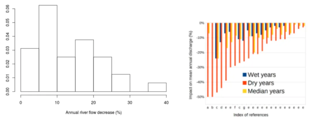
mately 30 references, the decrease in the mean annual discharge reaches 13.4% ±8% (Figure 1
73
and Appendix Table A.1).
74
Figure 1: Left: Distribution of the estimated annual stream discharge decrease attributed to reservoir networks. The distribution is established based on 20 values. Right: Impact on the annual discharge estimated during wet, median and dry years. Each bar corresponds to a different catchment. The estimations are from the following references: a: Gutteridge-Haskins-Davey (1987), b: Ockenden and Kotwicki (1982), c: Dubreuil and Girard (1973), d: Cresswell (1991), e: Teoh (2003), f: Habets et al. (2014), and g: Kennon (1966).
The right part of Figure 1 shows that the impacts on annual flows are not constant from year
75
to year but tend to be lower during the wet years and two times greater than the median impact
76
in the driest years. This result is very important because it indicates that even without changing
77
the small reservoir network, its impacts will change in the context of climate change: it may
78
decrease in areas that will become wetter but may increase in areas that will become drier.
79
One key issue in estimating the cumulative impacts is understanding how such impacts are
80
related to the reservoir network, i.e., the level at which the basin is equipped with small dams
81
to avoid over-equipping the basin, with consequences in terms of economy and ecology. Having
82
a single indicator or a set of indicators capable of estimating the cumulative impacts of small
83
reservoirs on the mean annual discharge would be helpful to most water management agencies.
84
Based on the estimated values collected in the literature, a preliminary analysis was performed
85
to determine whether some easy-to-access properties of the reservoir network could be used as
86
indicators. For this purpose, we collected the main characteristics of the basins and of their small
87
reservoir network from the available studies and attempted to connect them to the impacts on the
88
mean annual discharge. We used the reservoir’s density, expressed as the number of reservoirs
89
per square kilometre or as the volume stored per square kilometre, and the mean precipitation
90
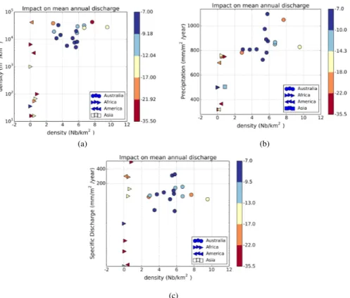
or the mean discharge in the basin. The results presented in Figure 2 show that none of these
91
characteristics are able to be used as indicators for such contrasted basins as the ones found in
92
the literature. Indeed, within a narrow range of specific discharge or precipitation, the decrease
93
of the annual discharge varies a lot and can not be correlated to the density of reservoir network.
94
A more regional-scale view could be useful to attempt to disentangle different types of
cli-95
mate or use. However, according to the sample of available studies, only a continental-scale
anal-96
ysis was possible. It appears from these figures that the general characteristics present a wider
97
spread between continents than within a given continent, even if the results are from different
98
studies. For instance, the specific discharge is low in Australia, the density is low in Africa, and
99
the storage volume tends to be important in America. However, even within a continent, these
100
characteristics are not sufficiently well linked to the impacts to be reliably used as indicators.
101
This result occurs because the cumulative impacts of reservoir networks rely on a large
num-102
ber of factors: the hydrological processes occurring in each reservoir, the water management
103
(water abstraction rate and timing, water uptakes from and releases to the river), the reservoir
104
characteristics, the reservoir network geometry, and the connectivity of each reservoir to the
105
stream drainage network. These points are detailed below.
(a) (b)
(c)
Figure 2: Cumulative impacts of the small reservoirs on the mean annual discharge (colour scale on the right), estimated from studies reported in Appendix Table A.1, as a function of possible indicators: reservoir density expressed as the number of dams per square kilometre and as storage capacity in cubic meter per square kilometre, annual precipitation expressed in mm/m2/year, or specific discharge expressed in mm/m2/year. Each point represents a catchment, and the
symbol corresponds to different regions: Africa, America, Asia, and Australia.
3. How do small reservoirs impact hydrology?
107
Small reservoirs have an impact on hydrology because they affect the natural water cycle that
108
would occur without reservoirs. To understand how networks of small reservoirs impact river
109
flow at the basin scale, it is necessary to understand the functioning of a single reservoir, how it
110
can have an impact on the river flow and why the impact varies in time and from one reservoir to
111
another.
112
3.1. Water balance of a small reservoir
113
Figure 3 presents the various terms of the water balance of the reservoir. From a general
114
perspective, the reservoir water balance can be expressed by the following equation:
115
Figure 3: Water balance of a small reservoir and its main drivers. The components of the water balance are indicated by large arrows: inputs can be inflows, such as upstream runoff, lateral surface runoff, and direct precipitation; outputs can be outflows, abstraction, seepage and evaporation.
dV
dt = Qin+ P + GWin− Qout− E − S − Qabs (1)
Here, dV is the water volume variation [m3] over the period dt [s], Qinis the stream inflow
116
to the reservoir [m3/s], Q
out is the outflow from the reservoir [m3/s], E is the evaporation rate
117
[m3/s], P is the precipitation rate [m3/s], S is the seepage rate [m3/s], GW
inis the groundwater
118
inflow [m3/s] and Q
absis the water abstraction [m3/s].
119
Inflow can have 4 sources: i) the upstream flow, which depends on the way in which the
120
reservoir is connected to the river (Section 3.3); ii) the surface runoff from the area directly
121
drained by the reservoir along its bank; iii) the intercepted precipitation; and iv) a groundwater
122
inflow, although none was reported in the literature review.
123
Outflux includes outflow (downstream flow) and water abstraction, as well as evaporation and
124
seepage losses from the reservoir. Outflow is defined as the downstream flow due to reservoir
125
release. Abstraction corresponds to the water uptake, often by pumping, for human use
(irriga-126
tion, livestock watering, and so forth). Seepage flow may occur as water infiltration through the
127
reservoir bed or through or below the dam.
128
All these fluxes can vary considerably from one reservoir to another. For instance, abstraction
can be the main output, especially for farm reservoirs. However, it can also be null, such as in
130
storm water or check dam reservoirs. Section 6.3 discusses how abstraction can be estimated at
131
the basin scale.
132
Water losses are present for every type of reservoir, but with a large spread of intensity,
133
ranging from the main outflux to negligible ones. The next section focuses on these losses and
134
on how they can be estimated.
135
3.2. Losses from small reservoirs
136
3.2.1. Seepage
137
Seepage (also called percolation flux) may be particularly important to consider for small
138
reservoirs because most of these reservoirs are built with earthen dams. The seepage rate depends
139
on the hydraulic head gradient between the reservoir and the underlying aquifer (or unsaturated
140
zone) or dam wall, as well as on the hydraulic conductivities of the aquifer and reservoir bed
141
material.
142
Although seepage is a loss at the reservoir scale, the water is not lost and is mostly diverted.
143
Indeed, infiltration tanks, encountered especially in Asia, are built to favour infiltration through
144
the reservoir bed to increase the groundwater recharge. In this way, a larger part of the monsoon
145
flow is stored in the groundwater while avoiding the evaporation loss from reservoirs during the
146
dry season (Glendenning et al., 2012). However, when dams are intended to store water over
147
the long term, seepage is considered as a loss. In such cases, impervious layers of clay or
ge-148
omembrane (Alonso et al., 1990; Yiasoumi and Wales, 2004) are used to reduce seepage, but
149
their efficiency decreases with age. Thus, irrespective of the intended function of the reservoir,
150
it is rather important to estimate the seepage rate from the reservoir because it determines its
ef-151
ficiency for storing water (then, a low seepage rate is expected) or within the groundwater (then,
152
a high seepage rate is expected). In the literature, estimations of the seepage rate were based on
153
water balance approaches constrained by local observations of the precipitation, potential
evapo-154
ration and reservoir’s water level (Culler, 1961; Kennon, 1966; Sukhija et al., 1997; Singh et al.,
155
2004; Bouteffeha et al., 2015), as well as on additional observations of the soil moisture and
156
piezometric heads (Shinogi et al., 1998; Antonino et al., 2005; Massuel et al., 2014),
environ-157
mental tracers (Sukhija et al., 1997), or more frequently on modelling approaches (Zammouri
158
and Feki, 2005; Boisson et al., 2014; Jain and Roy, 2017).
159
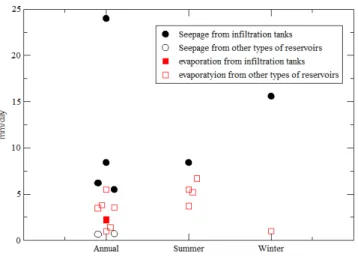
Figure 4 presents some estimations of the seepage and evaporation losses from the literature
160
under different hydroclimatic contexts and for reservoirs built for various purposes. Most
esti-161
mated seepage values are greater than 5mm/day on average in the studied periods, and thus, the
162
seepage rate appears to be higher than the evaporation rate. However, most of the values found
163
in the literature are from percolation tanks, i.e. from dams built to promote a rapid infiltration
164
of the runoff during the wet season to recharge the water table. For the other types of dams, the
165
estimations can be lower: less than 1mm/day for Culler (1961) in the US and up to 6.2mm/day
166
for Shinogi et al. (1998) over a 6-month period in a basin in Brazil. Fowler et al. (2012, 2015)
167
consider that hillslope dams in Australia are not efficient for storing water if the seepage rate is
168
greater than 5mm/day.
169
When the cumulative impacts are considered, both the seepage rate and the seepage fate are
170
important. In the case of infiltration into the dam wall, the seepage water might flow downstream
171
in the river, and thus, the seepage flux might not be lost at the scale of the river basin. An
illustra-172
tion of such a process was provided by Kennon (1966), who observed that ephemeral rivers have
173
become permanent after the implementation of dams built to prevent erosion (see Section 4.1.1),
174
and by those studies that include groundwater recharge from dam seepage (Ramireddygari et al.,
175
2000; Barber et al., 2009; Smout et al., 2010; Shinde et al., 2010; Perrin et al., 2012). Therefore,
176
seepage fluxes from each reservoir should not be aggregated to estimate the loss at the basin scale
177
and thus for the estimation of the cumulative impacts of small dams on hydrology.
178
3.2.2. Evaporation
179
Unlike seepage, evaporation fluxes from each reservoir should be aggregated at the basin
180
scale. The impact of the reservoirs on the evaporation losses is then the difference between the
181
evaporation from the land cover that was present prior to the dams being built and the
evap-182
oration from the reservoirs. Such estimations are not straightforward, particularly because the
183
heat storage of the water body affects the surface energy flux (Assouline et al., 2008;
McMa-184
hon et al., 2013). This storage partly depends on the temperature of the water columns, which
185
is impacted by the depth of the dams (although in opposite ways depending on the references
186
(Girard, 1966; Mart´ınez Alvarez et al., 2007; Magliano et al., 2015) due to the associated change
187
in the free water area); on the water circulation within the reservoir (which is also impacted by
188
the reservoir’s management); and on the interaction with the edges, which can be rather close
189
for small reservoirs and that affects the wind velocity and the advection of air humidity
(Fig-190
ure 3). Several methods were used to provide estimations of the evaporation from small
Figure 4: Estimation of the seepage loss and the evaporation flux of small reservoirs on a seasonal to annual basis. Two types of reservoirs are distinguished: infiltration reservoirs and other types of reservoirs. The values are taken from the articles cited in this section.
voirs based on observations: energy balance approaches (Anderson, 1954; Culler, 1961;
Ken-192
non, 1966; Gallego-Elvira et al., 2010), eddy-covariance measurements (Rosenberry et al., 2007;
193
Tanny et al., 2008; Mengistu and Savage, 2010; Nordbo et al., 2011; McJannet et al., 2013),
scin-194
tillometers (McJannet et al., 2013; McGloin et al., 2014), and water balance approaches (Girard,
195
1966; Mart´ınez Alvarez et al., 2007). Figure 4 presents the estimations found in the literature.
196
The mean annual estimations range from 1.4 to 5.5mm/day, and the reported summer values are
197
all above 3mm/day.
198
Mart´ınez Alvarez et al. (2007) proposed a relationship between the small reservoir
evapora-199
tion loss and the Class A pan evaporation that varies according to the reservoir’s depth and area
200
and that varies in time (from 86 to 94%).
201
Several estimations of the small reservoir evaporation loss based on meteorological data were
202
proposed (de Bruin, 1978; Mart´ınez Alvarez et al., 2007; McJannet et al., 2013; McMahon et al.,
203
2013; Morton, 1983). Benzaghta and Mohamad (2009), Mart´ınez Alvarez et al. (2008) and Craig
204
(2008) found that the evaporation losses from reservoirs can be very important at the regional
205
scale and have an important economic impact.
206
Several techniques might help reduce evaporation from reservoirs: casual chemical treatment
207
to modify the albedo or form a monolayer film, completely or partially covering the reservoirs,
208
managing the reservoir edges to reduce wind speed, and optimizing the use of the water in
reser-209
voir networks based on the temperature of the water in the reservoirs (Barnes, 2008; Lund, 2006;
210
Assouline et al., 2011; Mart´ınez-Alvarez and Maestre-Valero, 2015; Gallego-Elvira et al., 2011;
211
Carvajal et al., 2014; Reca et al., 2015). However, such techniques are not yet widely used and
212
are not considered in the existing cumulative impact studies.
213
3.3. Connection to the stream
214
By itself, the connection of the reservoir to the stream is key to understanding the impacts
215
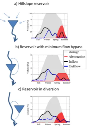
of the reservoir on the river flow. Indeed, this connection will impact both the inflow and the
216
outflow. Small reservoirs can collect all the upstream flow (Figure 5-a for a hillslope reservoir
217
or dam situated on the stream with no minimum flow) or only a part of the flow (reservoir
218
with minimum flow by-pass, Figure 5-b, which allows maintaining a minimum flow, or dam
219
situated in diversion Figure 5-c since in this case, the reservoir can not fill as long as inflow
220
does not exceed some thresholds). In the case that all the upstream flows are collected, the
221
downstream outflow will primarily depend on the level of the spill and on the reservoir water
222
storage. Following ”fill-and-spill” (Deitch et al., 2013), downstream discharge occurs only when
223
the reservoir is fully filled; conversely, as long as the reservoir has not reached its capacity,
224
downstream discharge is null. Therefore, it is possible to have periods with no downstream flow
225
while upstream flow exists, such as for hillslope reservoirs and check dams. Such reservoirs have
226
strong impacts on the intensity and the duration of low flows. In particular, the resumption of
227
flow in the fall can be significantly delayed. In the case of diversion or a minimum flow bypass
228
reservoir, a downstream flow is ensured when the upstream flow is non-zero. If the reservoir is
229
located in diversion, then the filling period of the reservoir can be managed such that the reservoir
230
may have no impact on the river flow during parts of the year, which may allow preserving
231
the ecological function of the river. This management can also be adapted to the hydrological
232
situation of each year. The reservoirs built mainly to favour groundwater recharge can have
233
all types of connections with the river; however, it appears that most of them are built directly
234
in the river stream, thus collecting all the upstream flows (Shinogi et al., 1998; Siderius et al.,
235
2015). Depending on the respective inflow and abstraction dynamics, cumulative abstraction
236
may exceed the reservoir storage capacity, as illustrated in Figure 5 for example, for which the
237
abstractions from the reservoirs reach 105 to 120% of the maximum storage capacity.
Figure 5: Illustration of 3 different connections between the river and the reservoir and its consequences in terms of river flow. Inflow, outflow and abstraction are accumulated weekly values, whereas storage is a weekly value. They are all expressed as a fraction of the maximum storage. Abstractions in the reservoirs reached 105 to 120% of the maximum storage capacity. a) Hillslope reservoir is managed as a fill and spill, with a weak and irregular inflow. b) The minimum flow bypass ensures that a minimum outflow occurs as long as inflow is present. c) The reservoir in diversion is expected to fill up as soon as the inflow reaches a given minimum flow or depending on management practices.
4. Methods to estimate the cumulative impacts of small reservoirs on hydrology
239
Quantifying the cumulative impacts of small reservoirs has been conducted using a variety
240
of methods, all of them requiring data and observations. Two classes of methods can be
distin-241
guished: i) the methods exclusively based on the analysis of observed data and ii) the methods
242
based on hydrological modelling.
243
4.1. Exclusively data-based methods
244
4.1.1. From observation of selected reservoirs to estimation of cumulative impacts
245
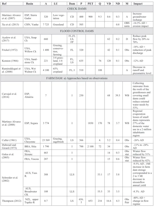
This approach was mainly used in early works performed from the 50s to the early 70s in the
246
US (Kennon, 1966; Culler, 1961; Frickel, 1972) and in Brazil (Dubreuil et al., 1968; Dubreuil
247
and Girard, 1973; Molle, 1991). In light of these pioneering works, it can be observed that the
248
cumulative impacts on hydrology have been a scientific and water management issue for a long
249
time.
250
Despite some differences in the methodology among these studies, they all aimed at
quantify-251
ing single reservoir hydrologic functioning from the monitoring of a sample of reservoirs. Losses
252
were estimated using a mass balance of the sampled representative reservoirs based at least on
253
the monitoring of the water level, inflows and outflows of the reservoirs. These early studies
254
initially made the assumption that cumulative reservoir impacts were the sum of the impact of
255
each reservoir following an aggregation process. However, the main outcome of these studies
256
was to show that this assumption was not valid. Indeed, Culler (1961) and Kennon (1966) found
257
that the seepage was a significant loss for the sampled reservoirs but contributed to downstream
258
flow. Therefore, interactions between reservoirs and hydrologic compartments, especially the
259
stream, were identified very early as processes to be taken into consideration to reliably estimate
260
the cumulative impacts.
261
4.1.2. Statistical analyses of the observed discharge
262
The idea is to connect the detected changes in the statistical properties of river discharge time
263
series with the evolution of the reservoir network within the basin. In doing so, the details of
264
each reservoir functioning are not taken into consideration. To our knowledge, this type of study
265
based solely on observations was only performed by Galea et al. (2005). A study based on a
266
30-year river discharge time series of two French catchments showed no stationarity break in
267
summer, while a break was shown in winter, i.e., during the filling period (Galea et al., 2005).
268
One difficulty of such statistical analyses is discriminating the specific impact of small
reser-269
voirs from those of land use and land cover (LULC) evolution or of climate change (CC).
Reser-270
voir development occurred over decades, a sufficiently long period to be sensitive to LULC
mod-271
ifications (such as agricultural intensification or crop modification) and CC. To overcome this
272
issue, Schreider et al. (2002) compared the observed river flows with simulated ones obtained
273
using the observed atmospheric forcing, but without any explicit representation of the small
274
dams in the models. The IHACRES rainfall-runoff model, a dynamic, lumped parameter model,
275
was used to simulate stream flow with parameters calibrated considering periods before the
de-276
velopment of reservoirs. They found significant decreasing trends in the observed discharge of
277
basins that had a development of farm dam capacity, and they were able to attribute these trends
278
to non-climatic stressors since such trends were not simulated with a reservoir-free basin.
4.1.3. Paired-catchment experiment
280
A paired-catchment experiment is an approach already used in hydrology for quantifying
281
the impact of LULC changes from a comparative analysis of stream flows monitored in two
282
contrasted catchments (see, for instance, Brown et al. (2005) for a review in forest hydrology).
283
Thompson (2012) is, to our knowledge, the only study using this approach to compare stream
284
flows from two adjacent and similar catchments, one without a reservoir and the second with
285
three small reservoirs. From an 18-month monitoring, annual stream flow was estimated to be
286
lower by 40% in the catchment with 3 reservoirs than in the ”no-reservoir” catchment
(Thomp-287
son, 2012). Although the experiment found differences in the specific discharge, the full
com-288
parison of the water balance remained difficult. The main shortcoming of Thompson’s approach
289
is that catchment properties (soils, lithology, land cover, topography, and so forth) were spatially
290
heterogeneous over a short distance, making deciphering the stream flow differences difficult.
291
Furthermore, indirect reservoir impacts on land use, such as the cattle grazing around the
reser-292
voir in Thompson’s case study, can also modify stream flow. The study would have benefited
293
from following the classic approach used in paired-catchment experiments, implying a
calibra-294
tion period where both catchments are monitored, followed by a period when one of the
catch-295
ments is subjected to land use change (reservoir building) and the other remains as a control.
296
However, building a reservoir network over a large area is generally difficult for practical and
297
financial reasons. Consequently, such an approach has never been utilized to our knowledge.
298
4.2. Modelling approaches
299
Modelling is the most widely used approach for studying and quantifying the cumulative
300
impacts of small reservoirs. Although various modelling approaches have been developed, all
301
are based on the coupling of the small reservoir water balance model with a quantitative method
302
to estimate stream inflow into the small reservoirs. Three of the main model components are
303
detailed below: i) the small reservoir water balance model, ii) the quantitative method used to
304
quantify inflow to reservoirs, and iii) the spatial representation of the reservoir network. The
305
inflow quantification method and the spatial representation of the reservoir have to be consistent
306
and are thus intrinsically dependent. A spatially distributed representation of reservoirs requires
307
being able to estimate the spatial distribution of stream flow to estimate the upstream inflow to
308
each reservoir. Conversely, an aggregated estimation of stream flow over a sub-basin or over
309
the full catchment leads to the reservoir network representation being aggregated on the same
310
domain.
311
Most of the reviewed studies focused on assessing the impacts of reservoirs used for irrigation
312
or livestock watering on stream flow. In such cases, the impacts are quantified by comparing the
313
catchment stream flow simulation with and without reservoirs, except for the TEDI model, as
314
we will see in Section 4.2.2. The exceptions to modelling approaches dedicated to stream flow
315
impacts are those aiming at assessing the impacts on groundwater. These approaches mostly
316
focus on infiltration tanks, for which part of the stored volume recharges the aquifer. In such
317
cases, only the impacts on the aquifer due to the loss from the reservoirs are represented, either
318
without simulation of the groundwater (Mart´ın-Rosales et al., 2007; Hughes and Mantel, 2010),
319
with a simplified representation of the aquifer (Smout et al., 2010; Shinde et al., 2010; Perrin
320
et al., 2012), or even more seldom, with a 2-D hydrogeological model (Ramireddygari et al.,
321
2000; Barber et al., 2009).
322
4.2.1. Reservoir water balance model
323
Reservoir water balance models rely on equation (1). Most small reservoir water balance
324
models take into account the evaporation and abstraction, for which temporal estimation is rarely
325
well known and is often an important point (see Section 5.3) (Table 1). When seepage is taken
326
into account, it is considered only as infiltration to groundwater. Ignoring seepage is justified
327
by the small expected rates (Hughes and Mantel, 2010) or by the lack of information on the
328
process (rate, timing, and driving factor G¨untner et al. (2004)) and by the fact that seepage flux
329
can contribute to downstream flow. To simulate the reservoir water mass balance, downstream
330
discharge is simulated considering that reservoirs operate with the technique of ”fill-and-spill”
331
(Section 3.3, unless a conservation flow is taken into account (Table 1). Reservoir inflow is
332
simulated by different approaches, as presented in the next section.
333
4.2.2. Reservoir inflow quantification
334
In most modelling approaches, upstream inflow is provided by a catchment hydrological
335
model simulating the water balance (WB), or the energy and water balance (EWB), in the
up-336
stream catchment and the routing of the flow downstream (Table 1). Existing catchment
hy-337
drological models are used in the modellings, reflecting the diversity of current hydrological
338
models. Such models need atmospheric forcing and some information on the land cover, soil and
339
topography, unless the model parameters are calibrated without any data on the physiographic
340
characteristics. Two models, TEDI and Deitch (Table 1), developed an alternative and pragmatic
method based on using observed discharge time series as input to the model. In doing so, the
342
TEDI and Deitch models do not belong to any current modelling approaches. Using observed
343
discharge at available river gauges implies being able to successively i) disentangle the natural
344
flow from the anthropogenic flow and ii) distribute the observed discharge along the reservoir
345
networks. To achieve the first step, Deitch et al. (2013) used historical gauged discharge
mea-346
sured prior to the reservoir pre-development period. The discharge was then spatially distributed
347
according to the drainage area of each reservoir and the spatial distribution of the average annual
348
rainfall. The propagation of stream water was then operated from the most upstream reach to the
349
catchment outlet by considering the water volume intercepted in each reservoir. The cumulative
350
impact of reservoirs is then classically the difference between simulated discharge and the gauged
351
discharge. In TEDI, Nathan et al. (2005) used the observed discharge of the period of interest.
352
The inflow in each reservoir is calculated from the observed catchment discharge assuming a
353
proportionality with the reservoir catchment area. The outflow from every reservoir is transfered
354
directly to the outlet. It is then considered that the obtained cumulative impact corresponds to
355
twice the simulated impact of the reservoir network because the gauge discharge already includes
356
the impacts of existing reservoirs.
357
4.2.3. Reservoir spatial representation
358
How the reservoir network is represented from a spatial perspective varies from one model to
359
another. The spatial representation of the reservoir network can be classified into the following
360
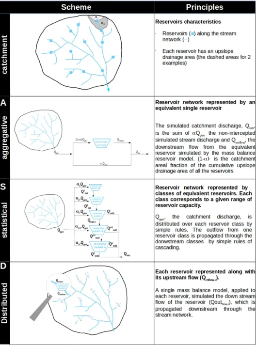
three types (see Figure 6, Table 1).
361
• In the spatially aggregate approach, all the reservoirs in a catchment (in Table 1, A for
362
aggregation on sub-catchments and A* for aggregation on a grid cell) are represented in
363
the form of a single equivalent, or composite, reservoir.
364
• The statistical representation constitutes a refinement of the aggregate representation
(Fig-365
ure 6-B). The reservoir network is represented in the model in an aggregated way by
group-366
ing reservoirs into a finite number of classes. Some hydrological connections between
367
several of these classes may be represented (S in Table 1).
368
• The spatially explicit representation consists of representing every reservoir (Figure 6-C).
369
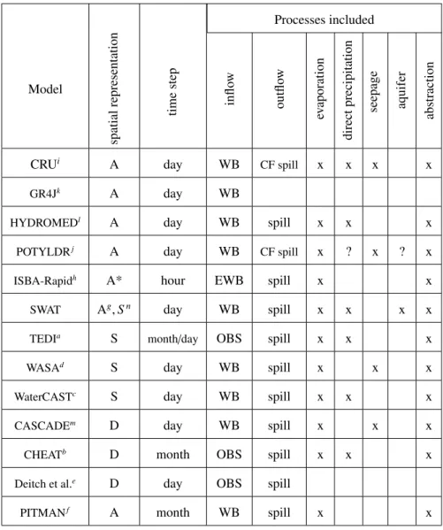
Processes included Model spatial representation time step inflo w outflo w ev aporation direct
precipitation seepage aquifer
abstraction
CRUi A day WB CF spill x x x x
GR4Jk A day WB
HYDROMEDl A day WB spill x x x
POTYLDRj A day WB CF spill x ? x ? x
ISBA-Rapidh A* hour EWB spill x x
SWAT Ag, Sn day WB spill x x x x
TEDIa S month/day OBS spill x x x
WASAd S day WB spill x x x
WaterCASTc S day WB spill x x x
CASCADEm D day WB spill x x x
CHEATb D month OBS spill x x x
Deitch et al.e D day OBS spill
PITMANf A month WB spill x x
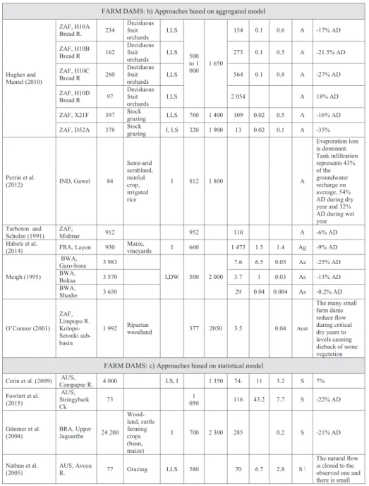
Table 1: Main processes in reservoir water balance model, as well as temporal and spatial representations of reservoirs in numerical models. Spatial representation can be the following (see Figure 6): A: aggregate representation by catchment (or A* by grid in grid-based models), S: statistical representation, or D: distributed representation. Inflow to the reservoirs can be derived from OBS: observations, WB: water balance, or EWB: energy and water balance. Outflow is computed either based on spill (above a water level or volume in the reservoir) and/or taking into account a conservation flow (CF).a: Nathan et al. (2005),b: Nathan et al. (2005),c: Cetin et al. (2009),d: G¨untner et al. (2004),e: Deitch et al.
(2013),f: Hughes and Mantel (2010),g: Perrin et al. (2012),h: (Habets et al., 2014),i: Tarboton and Schulze (1991),
j: Ramireddygari et al. (2000),k: Payan et al. (2008),l: Ragab et al. (2001),m: Shinogi et al. (1998); Jayatilaka et al.
Figure 6: Spatial representation of reservoir network in models used to quantify cumulative reservoir hydrologic impacts.
Aggregate representation
370
In the aggregate representation (Figure 6-A), the characteristics of the equivalent reservoir
371
(capacity and surface area) are obtained by aggregating single reservoir characteristics. The main
372
interest of the aggregate representation is to require only global information about the reservoirs
373
and their characteristics. In fact, the spatial density of reservoirs within a catchment can be large,
374
greater than 10 reservoirs/km2in some cases (Nathan et al., 2005), and an exhaustive inventory
375
of all reservoirs along with their characteristics is out of reach. Rather, a global estimation of
376
reservoirs and their characteristics may be approximated from simple rules of spatial
extrapola-377
tion (cf. Habets et al. (2014)). For instance, to estimate the inflow into the equivalent reservoir,
378
it is necessary to determine the contributive catchment. It can be a fraction of the catchment area
379
(Tarboton and Schulze, 1991; Hughes and Mantel, 2010) that can be estimated from the sum of
380
the drainage area of all reservoirs or depending on the cumulative reservoir area (Habets et al.,
381
2014).
382
The aggregate representation leads to obtaining a simulation of the hydrological
cumula-383
tive impacts of reservoirs at the catchment, grid-cell or sub-catchment outlet but intrinsically
384
does not allow simulating the cumulative impacts along the river network from the head to the
385
outlet, unless the sub-catchments are small, which is often not the case because the size of the
386
sub-catchment is often determined by the availability of river gauges. Furthermore, this
represen-387
tation may not reflect the different responses of the various reservoirs in terms of key processes
388
(evaporation, infiltration, operations, and so forth (Zhang et al., 2012)).
389
Statistical representation
390
The statistical representation is a trade-off between the other two representations. It
consid-391
ers that information about the location and characteristics of reservoirs, particularly of
small-392
and medium-sized reservoirs, cannot be exhaustively available. It also relies on the assumption
393
that reservoir connectivity may play a role in the cumulative impacts. The reservoir network
394
is represented by classes of reservoirs determined following reservoir water capacity (G¨untner
395
et al., 2004; Nathan et al., 2005; Lowe et al., 2005)) and also reservoir drainage area (Zhang et al.,
396
2012). Each class is represented as a single equivalent reservoir. G¨untner et al. (2004) and Zhang
397
et al. (2012) used a coupled sequential and parallel scheme to represent the upstream-downstream
398
connectivity of different water reservoir classes in the catchment.
399
As a main advantage, the statistical representation has to consider the diversity of key
voir processes, which can be variable from one reservoir to another but quite homogeneous in
401
reservoirs of similar sizes. In this way, it overcomes one of the main shortcomings of the
ag-402
gregate representation. Evaporation, for example, depends on the water column height and
cir-403
culation within the reservoir, which is expected to depend on reservoir size (cf. Section 3.2).
404
Connectivity to the network –reservoirs and rivers– and operation rules may also be different
405
depending on the reservoir function, which also depends on the reservoir size. Another
advan-406
tage of the statistical representation is being computationally faster than the fully distributed one
407
because fewer reservoir mass balances have to be computed and water transfers between
reser-408
voirs are simplified. The main shortcoming is that it does not obtain distributed simulations of
409
the hydrological impacts of reservoirs; particularly, the cumulative impacts along the full river
410
network cannot be simulated.
411
Distributed representation
412
A distributed representation of the reservoir is the only way to explicitly represent the
in-413
teractions between reservoirs by considering the outflow from one reservoir as a contribution to
414
the inflow of the downstream one and the interactions between reservoirs and hydrological
com-415
partments (river, soil, and aquifer) by estimating the impacts of each reservoir on its connected
416
river reach or/and aquifer. Indeed, two dams with similar characteristics may have different
im-417
pacts according to their location along the stream network, mostly because the inflow is not the
418
same. The interest in a spatially explicit representation is in quantifying and understanding the
419
local hydrologic impact at a river reach scale and the cumulative impacts along the river network
420
(Deitch et al., 2013). Quantifying local hydrologic impacts may be particularly relevant to water
421
quality, ecological disturbance or morphogenesis evolution. In a spatially explicit representation,
422
water inflow into every single reservoir as stream discharge and lateral surface runoff has to be
423
known or estimated. To our knowledge, only Shinogi et al. (1998) and Smout et al. (2010) have
424
performed catchment hydrologic modelling to obtain these estimations, with an application to
425
relatively simple case studies characterized by few reservoirs. Other reported case studies using
426
spatially explicit representations used observed-stream-discharge-based models (Nathan et al.,
427
2005; Cetin et al., 2009; Deitch et al., 2013).
428
A spatially explicit representation relies on the availability of exhaustive information about
429
reservoir location, characteristics, water uses and topology, which are rarely available over large
430
areas. This point constitutes a main shortcoming of the approach, as addressed in Section 4.1.1.
431
Furthermore, it can be expected that uncertainties in the local information, added to the
uncer-432
tainty in estimated spatial discharge and individual reservoir water balances, can skew the local
433
simulated impacts, and by propagation, the cumulative impacts. This could alleviate the
theoret-434
ical interest in the spatially explicit representation. Acknowledging the lack of information and
435
the difficulty to obtain it exhaustively, statistical representations and aggregate representations
436
are considered as pragmatical solutions and used in most modelling studies.
437
5. How to obtain access to the information needed on small reservoirs?
438
5.1. What type of data?
439
Stream discharge time series, at one or several points in the catchment, are required data
440
in statistical analyses (Section 4.1.2) and in the TEDI and Deitch models (Nathan et al., 2005;
441
Deitch et al., 2013, section 4.2.1), and such data are also used by the other types of models to
442
calibrate or assess the modelling. Such data are expected to be found in existing databases.
Sta-443
tistical analyses require rather long observation periods for both the discharge and the temporal
444
evolution of the reservoir network to cover contrasted periods. The modelling approaches
gen-445
erally need to collect more data, even if focusing on a shorter time period. These data include
446
atmospheric and physiographic data, as well as the characteristics of each reservoir (or of the
447
aggregated ones), the connection between the reservoirs, and the management of the reservoirs,
448
particularly in terms of abstraction. Table 2 presents some of the most commonly required data
449
on the reservoirs used for such studies.
450
5.2. Physical and topographical characteristics of small reservoirs
451
Data on small reservoir characteristics may be collected and stored in databases by
stake-452
holders or state or regional agencies. Although they are often a first base to initiate a study and
453
may prove very useful, such databases are generally incomplete, even for the census of the
reser-454
voirs, either because the survey did not include all the existing reservoirs or because the database
455
is not up to date. Moreover, all the needed data are not available. Therefore, to fill the gaps,
456
several methods can be used: i) additional field surveys, ii) remote sensing data (either satellite
457
or aerial images) and related image analysis techniques and iii) empirical relationships to recover
458
one variable according to other properties. In most studies, several methods are combined.
459
Here, only some indications on the available methods are presented because it is beyond
460
the scope of the present review to fully describe such techniques. Some details can be found
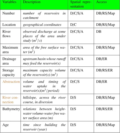
Variables Description Spatial repre-sentation
Access
Number number of reservoirs in
catchment
D/C/S/A DB/RS/Map
Location geographical coordinates D/C DB/RS/Map
River flows
observed discharge at some places of the area under study(m3/s)
D/C/S/A DB
Maximum area
area of the free surface wa-ter (m2)
D/C/S/A DB/RS/Map
Drainage area
upstream basin whose runoff may feed the reservoir(s)
D/C/S/A DB/ER
Storage capacity
maximum capacity volume of the reservoir(s) (m3)
D/C/S/A DB/RS/ER
Abstraction volume and timing of
water uptake in the
reservoir(s)(m3/period)
D/C/S DB/ER
River con-nection
hillslope, across the river course, in diversion
D/S DB/RS/Map
Bathymetry relations between height-water volume-height-water free wa-ter surface area (m)
D/S DB/RS/ER
Age time since building the
reservoir (year)
D/S DB/RS/Map
Table 2: Key variables needed to conduct a cumulative impact study of small reservoirs from the most common (top) to the less used (bottom). Spatialization can be either D: distributed, S: statistical, C: catchment or A: aggregated (see Figure 6). Access to the variables can be from DB: databases, RS: remote sensing (satellite data, aerial images, lidar and so forth), Map: mapping, or ER: empirical relationships (see subsection below). Variables in brown are associated with the management of the reservoir discussed in Section 5.2, whereas the other ones are discussed in Section 5.3.
in Nathan et al. (2005); Lowe et al. (2005); Hughes and Mantel (2010); Malveira et al. (2012);
462
Nathan and Lowe (2012); Bartout et al. (2015); Fowler et al. (2015).
463
Field surveys are not often described in the literature because they are quite basic. However,
464
field surveys represent a guaranteed method to locate all the reservoirs on a catchment and to
465
ensure their type of connection to the river. However, this method is time consuming and cannot
466
be used on large areas. The detection of reservoirs is efficient with remote sensing methods based
467
on aerial or satellite images, which allows retrieving both the number and areas of the reservoirs
468
(Chao et al., 2008; Messager et al., 2016). However, very small reservoirs (approximately 100m2)
469
are still difficult to detect, even with high-resolution aerial images (Carvajal et al., 2014).
470
Storage volume and bathymetry are more difficult to assess by remote sensing (Gal et al.,
471
2016), whereas uncertainty in the storage volume can lead to important error in impact studies
472
(Hughes and Mantel, 2010; Fowler et al., 2015). Thus, some empirical relationships are most
473
often used. Based on a geometrical analysis of a variety of reservoir shapes, Molle (1991) showed
474
that the relations between the reservoir surface and volume correspond to power laws. The
475
parameters of the laws vary in space, depending on the geomorphological context, but remain
476
generally constant within a given region (Thompson, 2012). Consequently, a common approach
477
is to fit the law parameters from a set of reference reservoirs. The law can then be applied to all
478
reservoirs in the catchment (Malveira et al., 2012; Hughes and Mantel, 2010).
479
The drainage area of the reservoirs can be derived from digital terrain models. However, this
480
requires having a precise position of the reservoirs to be able to connect them with the correct
481
river reaches to avoid error in the estimation of the upstream drainage area (Hughes and Mantel,
482
2010). Moreover, the determination of the type of connection between the reservoir and the river
483
is a key point for assessing how the reservoir is filled. For modelling approaches that are not
484
fully distributed, it is possible to use some relationship between the free surface water area (or
485
volume) and the drainage area of the reservoir. Linear (Habets et al., 2014; Nathan et al., 2005)
486
or non-linear (Fowler et al., 2015) relationships have been used. However, these relationships are
487
again often specific to the studied catchment and cannot be generalised to very different contexts.
488
5.3. Water reservoir management characteristics
489
Water reservoir management operations refer to how the volume is stored in the reservoir
490
and released from the reservoir either downstream, outflow, or withdrawn for some usage (most
491
often, agricultural use). The type of reservoir-stream connection is an important driver for such
management, as shown in Section 3.3. Information on the connection can be included in some
493
databases managed by stakeholders or regional agencies, particularly where legal regulations
ex-494
ist, for instance, to maintain a conservation flow. However, as stated previously, such databases
495
are often incomplete. Hughes and Mantel (2010) show that it is difficult to obtain this
informa-496
tion from remote sensing. Covering all the small reservoirs with a field survey is also difficult;
497
such information is thus likely to be incomplete. This is perhaps the reason why most existing
498
studies do not consider the ability to disconnect the small reservoirs from the stream network
499
or to maintain some minimum flow by some type of diversion canal or low-flow bypass. Some
500
exceptions are the works of Fowler et al. (2009) and Thompson (2012) that considered low-flow
501
bypasses and of Habets et al. (2014) that considered the possibility to disconnect the reservoirs
502
during part of the year (as if they were in diversion) to manage a filling period as required by
503
the regional regulation. However, a limitation is that in these cases, the management operations
504
were supposed to be homogeneous within the basin.
505
Water abstraction is the most sensitive information needed to infer the cumulative impacts
506
of small reservoirs on hydrology (Hughes and Mantel, 2010; Fowler et al., 2015). However, the
507
abstraction is rarely known, and at best, only an annual estimation of the abstracted water volume
508
is known. To retrieve the temporal evolution of the water abstraction, which of course varies from
509
year to year, several methods are used in the literature, either based on the estimation of the water
510
demand or on the water offer (i.e. the available water volume stored in the reservoirs).
511
Water demand approaches attempt to quantify the needs associated with irrigating crops and
512
watering livestock. Consumption for watering livestock is considered to be constant
through-513
out the year (Fowe et al., 2015), whereas irrigation is estimated according to the sub-seasonal
514
climate conditions. The water demand of the crop is often calculated on the basis of the crop
515
coefficient Kc, which varies over time, and potential evapotranspiration (PET) (Fern´andez et al.,
516
2007; Wisser et al., 2010; Biemans et al., 2011; Fowe et al., 2015).
517
Water offer approaches consider that the abstraction accounts for a given fraction of the total
518
reservoir capacity. This approach is mainly used in Australia (Nathan et al., 2005; Cetin et al.,
519
2009; Fowler et al., 2015). The fraction of the total storage can be obtained through surveys of
520
reservoir owners or occasionally by remote detection (Fowler et al., 2015) and is highly variable
521
depending on usage (irrigation vs. watering livestock) and region. Nathan and Lowe (2012)
522
refers to fractions ranging from 10% to 400%, which implies that the reservoir can be filled
523
several times within a year. Although rather simple, this method allows considering a seasonal
524
distribution of the abstraction according to known uses (Cetin et al., 2009). This method can
525
also be used when no information on the abstractions is available simply by assuming that the
526
abstraction volume is a given fraction of the storage capacity (Habets et al., 2014; Deitch et al.,
527
2013).
528
6. Discussion
529
6.1. The uncertainty issue
530
Regardless of the approach (exclusively data-based method or modelling approaches), stream
531
flow is a crucial variable in any reservoir impact estimation and may be a source of uncertainty
532
in cumulative impact estimation. The uncertainty arises from uncertain measurements of stream
533
flow, including the need to transpose data from neighbouring catchments, as well as from time
534
series that are too short. It can lead to incorrect conclusions in trend analysis within
statisti-535
cal analyses of time series (Section 4.1.2) and in comparisons of paired-catchment hydrology
536
(Section 4.1.3).
537
In modelling approaches, when catchment models are used to simulate inflow to reservoirs
538
and transfer of reservoir outflow to the outlet, uncertainties in cumulative impact simulations
539
derive from uncertainties classically associated with catchment hydrologic models, namely, the
540
model itself (structure and parameters) and the data used to calibrate and validate the model. An
541
extensive presentation and discussion of these sources of uncertainty are beyond the scope of
542
the present review and can be found elsewhere (see, for instance, Hingray et al. (2009)). When
543
observed discharge is used rather than hydrologic catchment models, as in Deitch’s model, in
544
TEDI or in CHEAT, the simplifications performed to spatialize observed discharge as reservoir
545
inflow may result in strong errors in reservoir dynamics, in outflow simulation and thus in
cu-546
mulative impact estimation. The assumption used to aggregate reservoir outflow may also be
547
another source of uncertainty. To our knowledge, no sensitivity and uncertainty analyses of the
548
simplifications and assumptions have been performed.
549
How the reservoirs are accounted for in the models, together with how the hydrological
550
processes are estimated, are key components of the models. Incorrect representations may lead
551
to significant uncertainty in the estimation of cumulative impacts. Indeed, processes and factors
552
that affect reservoir water balance (Section 3.1) and thus cumulative impacts (Section 4.2) are
numerous. In the approaches for quantifying cumulative impacts, choices are made irrespective
554
of the key processes and their representation; seepage, for instance, is often neglected (Table
555
1). The reservoir network representations (Table 1) in models also vary from one approach to
556
another. The physical, topographic and management characteristics of reservoirs (Table 2) may
557
also have uncertainties due to a lack of information or measurement and survey errors. The
558
uncertainty in the estimation of cumulative impacts is thus a key issue.
559
A few modelling studies have addressed this issue by conducting sensitivity analyses
(Ha-560
bets et al., 2014; Hughes and Mantel, 2010; Malveira et al., 2012; Nathan et al., 2005). Although
561
incomplete, three preliminary results can be emphasized. a) The effect of the uncertainty on the
562
estimated upstream drainage area of reservoirs on inflow is controversial. On the one hand, it
563
was shown to be a key morphological characteristic. This would have to be expected as the larger
564
the upstream drainage area is, the larger the flow intercepted by reservoirs (Habets et al., 2014;
565
Hughes and Mantel, 2010). On the other hand, the stream flow was shown to not be very
sensi-566
tive to the reservoir drainage area (Nathan et al., 2005). The hydrologic characteristics (annual
567
flow, monthly flow, and flow duration curves) taken into consideration to evaluate the cumulative
568
impacts may explain the differences between these findings. b) Water management of reservoirs
569
appears to play a dominant role in stream flow reduction. This was clearly shown by Hughes and
570
Mantel, quantifying the key role of water demand uncertainty confirmed by G¨untner et al. (2004),
571
stating that ”local experience suggests that uncertainty in human withdrawal add the largest
un-572
certainty”. c) Nathan et al. (2005) found that for the studied Australian catchments, the spatial
573
representation of reservoirs, especially the topology and the cascading between reservoirs, does
574
not exert a great role on stream flow reduction within the range of reservoir distribution.
575
From these preliminary conclusions, we highlight in the two following sections the need and
576
the ways to improve knowledge of reservoir characteristics and estimate water abstraction from
577
reservoirs. Uncertainty derived from process representations also deserves a thorough analysis,
578
particularly how reservoir evaporation is quantified and the consequence of neglecting seepage
579
in most of the approaches. It is expected that the sensitivity and uncertainty propagation may be
580
different as functions of the hydrologic characteristics used to assess the cumulative impacts.
581
6.2. Improving knowledge of small reservoir characteristics
582
Estimating the cumulative impacts of small reservoir networks requires obtaining the key
583
physical and geometrical characteristics of networks and reservoirs (Table 2). Unlike large
reser-584