Chandra View of Magnetically Confined Wind in HD 191612: Theory versus
Observations
Ya¨el Naz´e
1,2GAPHE - STAR - Institut d’Astrophysique et de G´eophysique (B5C), Universit´e de Li`ege, All´ee du 6 Aoˆut 19c, 4000-Li`ege, Belgium
Asif ud-Doula
Penn State Worthington Scranton, Dunmore, PA 18512, USA and
Svetozar A. Zhekov
Institute of Astronomy and National Astronomical Observatory, 72 Tsarigradsko Chaussee Blvd., Sofia 1784, Bulgaria
ABSTRACT
High-resolution spectra of the magnetic star HD 191612 were acquired using the Chandra X-ray ob-servatory at both maximum and minimum emission phases. We confirm the flux and hardness varia-tions previously reported with XMM-Newton, demonstrating the great repeatability of the behavior of HD 191612 over a decade. The line profiles appear typical for magnetic massive stars: no significant line shift, relatively narrow lines for high-Z elements, and formation radius at about 2R∗. Line ratios confirm the softening of the X-ray spectrum at the minimum emission phase. Shift or width variations appear of limited amplitude at most (slightly lower velocity and slightly increased broadening at minimum emission phase, but within 1–2σ of values at maximum). In addition, a fully self-consistent 3D magnetohydrody-namic (MHD) simulation of the confined wind in HD 191612 was performed. The simulation results were directlyfitted to the data leading to a remarkable agreement overall between them.
Subject headings:stars: early-type – stars: winds – X-rays: stars – stars: individual: HD 191612
1. Introduction
Classified as Of?p nearly half a century ago (Wal-born 1973), HD 191612 regained interest only a decade ago when large variations of its line profiles were identified (Walborn et al. 2003). As in HD 108, another Of?p star (Naz´e et al. 2001), strong narrow emissions, especially in H,He i lines, practically disap-pear at certain times. A photometric period of ∼537d was then identified for HD 191612, thanks to Hippar-cos photometry (Koen & Eyer 2002; Naz´e 2004), and it was readily shown to be consistent with the
spectro-1FNRS Research Associate 2naze@astro.ulg.ac.be
scopic changes (Walborn et al. 2004; Howarth et al. 2007). Moreover, variations of the X-ray flux (Naz´e et al. 2007, 2010) and UV line profiles (Marcolino et al. 2013) were detected, and found to occur in phase with those in the visible range. Finally, HD 191612 became the second O-star with a detected (strong) magnetic field (Donati et al. 2006; Wade et al. 2011). Currently, there are about a dozen known O stars with detectable global magnetic field (Fossati et al. 2015; Wade et al. 2016).
The field detection appeared as a key to understand the star’s peculiarities. Indeed, such a strong magnetic field is able to channel the stellar winds from opposite hemispheres towards the equatorial regions, forming
a disk-like feature. This slow-moving, dense material generates narrow emissions in the visible range (no-tably in H,He i lines). The variations detected at optical wavelengths could be closely reproduced with magne-tohydrodynamic (MHD) models simply by changing the angle-of-view on the confined winds (Sundqvist et al. 2012). Indeed, when the rotation and magnetic axes are not aligned, our view towards these magnetically-confined winds changes with time. This can also ex-plain the behavior in UV as confined winds seen edge-on are able to produce the larger absorptiedge-on at low ve-locities seen in the UV profiles (Marcolino et al. 2013). Finally, the collision between the wind flows is able to produce multi-million degree plasma, generating X-ray emission (Babel & Montmerle 1997a). Depending on geometry, some occultation may occur as the stellar body comes into the line-of-sight towards the confined winds at some (rotational) phases.
While improvements in our understanding of con-fined winds have been tremendous in the last decade, several aspects remain to be explained. To further gain insight on the hottest plasma in magnetospheres, high-resolution X-ray spectra with different angles-of-view on the magnetosphere are needed. Few strongly mag-netic O-stars can be studied this way, however. Most objects (e.g. NGC1624-2 Petit et al. 2015, CPD – 28◦2561 Naz´e et al. 2015, HD 57682 Naz´e et al. 2014, Tr16-22 Naz´e et al. 2014) are much too faint for such an endeavor, while others have more practical prob-lems - e.g. the long period (about 55 yrs, Naz´e et al. 2006) of HD 108 prohibits a study of its variabil-ity over the lifetime of X-ray satellite missions. Cur-rently, a high-resolution spectral analysis of confined winds is thus possible only for three stars: θ1Ori C, HD 191612, and HD 148937.
The latter object, discussed in Naz´e et al. (2012, 2014), has a constant X-ray emission, linked to a quasi unchanged view of its magnetosphere (always seen near pole-on) which limits the available information. High-resolution spectral analysis of the O star θ1Ori C is also available (e.g. Schulz et al. 2003; Gagn´e et al. 2005). In particular, Gagn´e et al. (2005) showed that ‘magnetically confined wind shock’ (MCWS) paradigm (Babel & Montmerle 1997a) was clearly at work even in an O star. However, their analysis was based on, although fully self-consistent, 2D MHD simulations which naturally impose an artificial az-imuthal symmetry. Furthermore, they compared their numerical models to the observational data only in-directly: for example, temperatures and line widths
derived from XSPEC fits were confronted to values independently estimated from simulation outputs – the numerical model itself was never directly fitted to the observational data to judge its adequacy.
Work here reflects further improvements in sev-eral aspects. A Chandra monitoring of HD 191612 at high-resolution allows us to see the hottest mag-netospheric component under different angles, lead-ing to precise observational constraints of its prop-erties. We present the first fully self-consistent 3D MHD model of HD 191612. Relying on the dynami-cal output of this numeridynami-cal model, we use a dedicated XSPEC model to make a direct comparison between the theory and observations.
In the next section, we present the observations and their reduction. This is followed by a discussion of our 3D MHD model. We then present the results, in-cluding the direct comparison between the observa-tions and our models, in §4, and we summarize our results in §5.
2. Observations and data reduction
High-resolution spectroscopy of HD 191612 was acquired with Chandra-HETG at two key phases, the maximum and minimum emission phases. These phases correspond to specific angles-of-view onto the confined winds. Indeed, Wade et al. (2011) derived β + i = 95 ± 10◦ (with i the inclination angle and β the obliquity of the magnetic axis relative to the rotation axis), while Sundqvist et al. (2012) showed that β = i yielded the best fit to the variations in the strength of Hα emission component. Thus, the maxi-mum emission phase corresponds to a pole-on view of HD 191612, with confined winds seen face-on, while minimum emission corresponds to an equatorial view, with confined winds disk-like structure seen edge-on.
The maximum was covered by four exposures in May-July 2015 totaling 142 ks, while the observation at minimum was split over 6 exposures in early 2016 totaling 196 ks (Table 1). The HEG (resp. MEG) count rates are 0.0061 (resp. 0.014) cts s−1at maximum and 0.0046 (resp. 0.0095) cts s−1at minimum: the different exposure times thus allow us to have data of similar quality (with ∼ 900 and 2000 cts for HEG and MEG, respectively) at both phases, facilitating comparisons.
The data were processed using CIAO v4.8 and CALDB v4.7.0. After the initial pipeline process-ing (task chandra repro), the high-resolution spec-tra of each set were combined using the task
com-bine grating spectra, also adding +1 and −1 orders. In addition, for each exposure, the 0th order spectrum was extracted in a circle of radius 10px (corresponding to 5”) around the Simbad position of the target while the associated background was evaluated in the sur-rounding annulus with an outer radius of 30px. Dedi-cated response matrices were calculated using the task specextract. The spectra and matrices were then com-bined using the task combine spectra to get a single spectrum for maximum and one for minimum. At the maximum emission phase, the count rate of the 0th or-der spectrum amounts to 0.014 cts s−1, whereas it is 0.0095 cts s−1 at minimum. Further spectral analysis was performed within XSPEC v12.9.0i. Note that, for broad-band fitting, all spectra were grouped to reach a minimum of 10 counts per bin.
3. 3D MHD Model
In our procedure to simulate the wind of HD 191612 fully self-consistently in 3D, we simply adopted the known stellar parameters of HD 191612 (Table 2, Sundqvist et al. 2012), in order to see how well a detailed, independent simulation of the confined wind based solely on the stellar parameters reproduces X-ray observations. There were no special adjustments to any of the parameters.
Our basic methods and formalism for MHD model-ing closely follow ud-Doula & Owocki (2002) along with Gagn´e et al. (2005) which includes a detailed energy equation with optically thin radiative cooling (MacDonald & Bailey 1981). The computational grid and boundary conditions are nearly identical to the ones presented in ud-Doula et al. (2013) for θ1Ori C except for the larger extent in radius that now goes from 1R∗ to 20R∗ to accommodate for the stronger magnetic field in HD 191612. The radiation line force is calculated within the Sobolev approximation using standard CAK (Castor et al. 1975) theory using only the radial component of the force. Since the rotation of HD 191612 is extremely slow (period of 537.2 d, Wade et al. 2011), rotational effects on the dynamics of the wind are expected to be negligible. As such, our model assumes no rotation, and equator throughout this paper will refer to magnetic equator.
Using only adopted stellar parameters, we first relax a non magnetic, spherically symmetric wind model to an asymptotic steady state. This relaxed wind model is then used to initialize density and velocity for our 3D MHD model. For the initial magnetic field, we
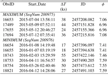
Table 1: Journal of the Chandra observations, ordered by ObsID, with their associated phase according to the ephemeris of Wade et al. (2011).
ObsID Start Date ∆T JD φ
(ks) MAXIMUM (SeqNum 200975) 16653 2015-07-04 13:58:11 38 2457208.082 7.06 17489 2015-05-09 07:52:11 44 2457151.828 6.96 17655 2015-05-12 20:46:27 24 2457155.366 6.96 17694 2015-07-12 07:35:41 36 2457215.816 7.08 MINIMUM (SeqNum 200976) 16654 2016-01-08 14:19:48 17 2457396.097 7.41 16655 2016-01-07 03:19:19 18 2457394.638 7.41 18743 2016-02-03 15:29:59 55 2457422.146 7.46 18753 2016-04-11 16:54:57 30 2457490.205 7.59 18754 2016-03-26 02:40:46 50 2457473.612 7.55 18821 2016-04-12 14:28:06 27 2457491.103 7.59
Fig. 1.— A sample view of our 3D MHD model of the star showing an iso-density surface (log(ρ)= −15, with ρ in g cm−3) colored by logarithm of temperature (in K) at an arbitrary time, t=2 Ms (end of simulation). Note clearly cool material along the pole, and mostly hot confined wind near the equatorial region. Unlike in 2D MHD models, there is no azimuthal symme-try here, and wind has a range of temperature as visi-ble in this color figure along with numerous scattered dense clouds. Outline of a semi-circle represents the full computational domain extending from 1 to 20 R∗, providing a rough scale for comparison.
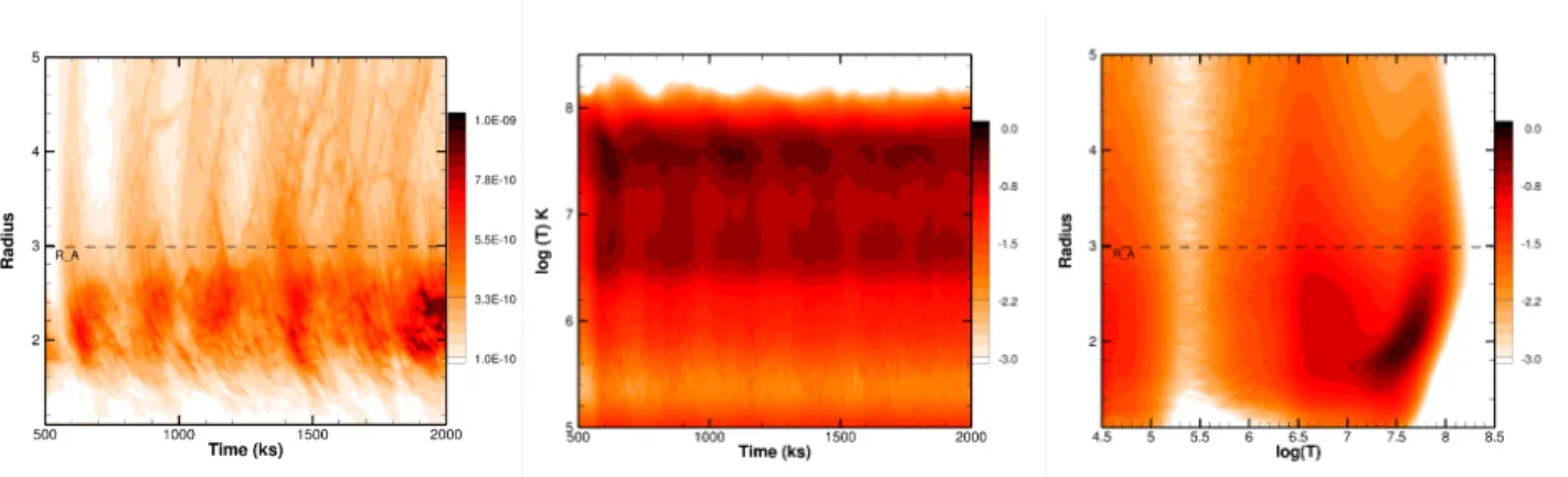
Fig. 2.— Left: The radial distribution of mass, dme/dr integrated over full azimuth, plotted versus time and radius (in units of R∗). The color bar shows dme/dr in units of M /R∗. The horizontal dashed line denotes Alfv´en radius RA. As evident by a darker band, the magnetosphere is limited within this radius, with the main plasma component located at 1.6–2.8 R∗. Middle: Distribution of emission measure, E M(t, T ), plotted with a logarithmic color scale (normalized to the peak value) versus simulation time (in ks) and logarithm of temperature log(T ) (in K). After an initial transient phase, the plasma distribution appears stable with large volume of gas in the temperature range of 106.4-107.6K. Right: Time-averaged distribution of emission measure, E M(r, T ), plotted with a logarithmic color scale (normalized to the peak value) versus radius (in units of R∗) and logarithm of temperature log(T ) (in K). It demonstrates that most of the hot and dense gas, source of X-rays, is located within 1.6–2.8 R∗.
assume an ideal dipole field with components Br = Bo(R∗/r)3cos θ, Bθ = (Bo/2)(R∗/r)3sin θ, and Bφ= 0, with Bo the polar field strength at the stellar surface. From this initial condition, the numerical model is then evolved forward in time to study the dynamical com-petition between the field and flow.
The effectiveness of field in channeling wind ma-terial depends on its relative strength to wind kinetic energy, and can be characterized by a dimensionless “wind magnetic confinement parameter” (ud-Doula & Owocki 2002), η∗≡ B2 eqR2∗ ˙ Mv∞ , (1)
where for a dipole, the equatorial field is just half the polar value, Beq = Bo/2. In the case of HD 191612, η∗ ≈ 50 >> 1 and the magnetic field dominates the wind outflow near the stellar surface up to a character-istic Alfv´en radius, set approximately by ud-Doula et al. (2008):
RA R∗
≈ 0.3+ η1/4∗ ≈ 2.95 . (2) Since the magnetic field energy falls off much more steeply than the wind kinetic energy, the wind can open the field lines above this radius.
After a short initial transient phase (<500 ks), the
simulation settles into a quasi-steady state wherein wind along the poles flow freely whereas material within magnetosphere shocks, cools and then falls back onto the stellar surface in a random fashion, very similar to what happens for the case of θ1Ori C (ud-Doula et al. 2013). Fig. 1 provides a glimpse of this dynamical interaction between the field and the wind: cool polar wind is apparent whereas hot dense mate-rial is located around the equator. The clumpiness of the hot confined winds is reminiscent of that observed for their cooler component (Sundqvist et al. 2012; ud-Doula et al. 2013); it has limited impact on the global properties (X-ray brightness, line profiles,...), as the temporal analysis of the simulations shows.
To facilitate the understanding of the time evolution of this numerical model, let us follow the approach by ud-Doula et al. (2013) wherein they define an equato-rial radial mass distribution as a function of time:
dme dr (r, t)= 1 2π Z 2π 0 Z π/2+∆θ/2 π/2−∆θ/2 ρ(r, θ, φ, t) sin θ dθ dφ (3) where∆θ = 10◦ represents a cone around the equa-tor. The left panel of Fig. 2 shows this equatorial mass distribution averaged over the azimuth. Clearly, large amount of mass is trapped within the magnetosphere limited by the Alfv´en radius, RA. Unlike in 2D
mod-els where there are clear episodes of emptying and re-filling of the magnetosphere, in 3D, on average there is a nearly constant amount of material trapped in the magnetosphere within 1.5 − 3R∗. The middle panel of the same figure shows the differential emission mea-sure (DEM) as a function of simulation time and tem-perature, demonstrating the near constancy of hot gas, while the right panel shows the DEM but this time as a function of radius and temperature, demonstrating that most of the hot gas is located within the magneto-sphere at ∼ 1.6 − 2.8R∗.
3.1. Predicted X-ray line profiles
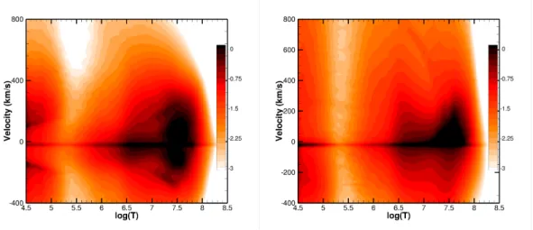
Our fully self-consistent dynamical model allows us to synthesize X-ray line profiles. First, we compute the line-of-sight velocity distribution of the plasma at both phases (pole-on for the maximum emission phase and equator-on for the minimum) as a function of tem-perature by assuming optically thin wind. To avoid any contamination from initial condition transients, the distributions were time-averaged from 500 ks to 2000 ks.
The resulting profiles are shown in Fig. 3, while Fig. 4 compares the line profiles obtained at both phases for selected plasma temperatures. The line shift of the simulated profiles is always close to zero (around −20 km s−1) and it is the same at the two phases. Because the plasma is strongly confined near the magnetic equator, the FWHMs always appear quite narrow, about 30 km s−1, but extended wings exist, reaching up to 300km s−1on each side. These wings reach larger velocities for log(T )= 7.7 or at the maxi-mum emission phase.
Table 2: Stellar parameters used for the MHD model, from Sundqvist et al. (2012).
Parameter Value Te f f 35 kK log g 3.5 R∗ 14.5 R v∞ 2700 km s−1 ˙ M 1.6 × 10⁻⁶M yr−1 Bo 2.45 kG
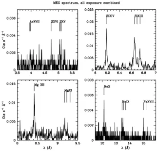
Fig. 5.— MEG spectrum combining all Chandra ex-posures, with lines labelled.
Fig. 3.— The panels show the plasma velocity (in km s−1) distribution as a function of plasma temperature, with colors representing E M(v, T ) in logarithmic units (normalized to the peak value). The left panel represents the maximum emission phase (pole-on view) while the right one corresponds to the equatorial view (minimum emission phase).
Fig. 4.— Comparison of the simulated line profiles at selected temperatures (pole-on view in black solid line, equator-on view in dashed magenta line). Note that the emissivity peaks of the Si f ir triplet and Lymanα lines occur at log(T )= 7.0 and 7.2, respectively.
4. Results
4.1. Line-by-line analysis of X-ray lines
The high-resolution HEG/MEG spectra reveal the typical lines of massive stars’ spectra: f ir triplets as-sociated to the He-Like ions of Ar (barely detectable), S, Si, Mg, and Ne, as well as Fe xvii lines near 15Å and Lymanα lines of H-like S, Si, Mg, and Ne (see Fig. 5). The H-like lines of Mg and Si appear stronger than the He-like lines of the same elements, while H-like and He-like lines of S display similar strengths. Such fea-tures are untypical for “normal” O-stars which rather show very faint or undetectable Mg xii, Si xiv, or S xvi lines, but they were already seen in HD 148937 and θ1Ori C (Naz´e et al. 2012, see in particular their Fig. 2 for a graphical comparison of X-ray spectra from nor-mal and magnetic O-stars). This underlines the pres-ence of hot plasma in magnetic stars.
Not all lines have enough counts to provide a mean-ingful fit, however. Only the strong X-ray lines in the 5–12Å range were fitted by Gaussians, using Cash statistics and unbinned spectra. Fitting was simulta-neously performed on both HEG and MEG spectra, to increase signal-to-noise. For Lymanα lines, two Gaus-sians are used: the two components were forced to share the same velocity and width, and their flux ratio was fixed to the theoretical one in ATOMDB1. For f ir triplets, four Gaussians were used, sharing the same velocity and width, and the flux ratio between the two intercombination lines was again fixed to the theoret-ical one. No background subtraction was done before fitting: a simple, flat power law being used to represent the local background around the considered lines. Ta-ble 3 yields the line properties measured for both the maximum and minimum phases, with 1σ errors deter-mined using the error command under XSPEC.
No significant line shift is detected, as expected (Figs. 3, 4) but also as seen in the XMM-Newton data of HD 191612 (Naz´e et al. 2007) or in the Chandra data of θ1Ori C (Gagn´e et al. 2005) and HD 148937 (Naz´e et al. 2012). Averaging across the five line sets yields a mean velocity of 68±44km s−1at maximum flux and 4±46km s−1at minimum flux. This slightly larger redshift at maximum, when confined winds are seen face-on, is contrary to what was observed for the average line shift of θ1Ori C (where the mean radial velocity changed from −75 to 93km s−1 at the same phases) - but the errors are large, requiring
confirma-1See e.g. http://www.atomdb.org/Webguide/webguide.php
Table 3: Properties of the X-ray lines, with 1σ errors.
Line Max Min
Lymanα lines Si xiv v(km s−1) 0±63 0±88 FWHM (km s−1) 399±300 871±231 Fx(10−6ph cm−2s−1) 4.58±0.39 2.78±0.34 Mg xii v(km s−1) 79±90 33±68 FWHM (km s−1) 351±224 557±170 Fx(10−6ph cm−2s−1) 3.05±0.59 1.88±0.34 Ne x v(km s−1) 68±123 −47±44 FWHM (km s−1) 776±327 52±233 Fx(10−6ph cm−2s−1) 5.25±1.28 4.25±0.91 He-like triplets S xv v(km s−1) 95±133 181±158 FWHM (km s−1) 780±338 unconstrained Fx( f ) (10−6ph cm−2s−1) 2.06±0.60 0.41±0.30 Fx(i) (10−6ph cm−2s−1) 0.15±0.42 0.51±0.34 Fx(r) (10−6ph cm−2s−1) 2.66±0.63 0.90±0.39 f/i 13.9±39.3 0.80±0.80 f+ i/r 0.83±0.34 1.02±0.67 Si xiii v(km s−1) 100±67 −148±112 FWHM (km s−1) 524±161 1239±203 Fx( f ) (10−6ph cm−2s−1) 1.45±0.33 1.75±0.34 Fx(i) (10−6ph cm−2s−1) 1.45±0.37 0.79±0.42 Fx(r) (10−6ph cm−2s−1) 3.91±0.50 3.09±0.47 f/i 1.00±0.34 2.22±1.25 ( f + i)/r 0.74±0.16 0.49±0.09
tion. If this occurs, then it would constitute another difference in behavior between HD 191612 (and more largely Of?p stars) and θ1Ori C, along with the known differences in X-ray hardness and in its variations (the very hard X-rays of θ1Ori C somewhat soften while brightening, opposite to the behavior of the softer X-ray emission of HD 191612 Naz´e et al. 2007, 2014), as well as in UV lines (opposite behavior in C iv and N v, see e.g. Marcolino et al. 2013; Naz´e et al. 2015): it might help us understand the physical origin of this (still unexplained) difference.
The X-ray lines detected in HETG generally appear resolved, with FWHMs of 400–1200km s−1. The ob-served profiles indicate broader FWHMs than simula-tions (Figs. 3, 4), a problem already encountered for θ1Ori C (Gagn´e et al. 2005) though with a lesser am-plitude. Observed lines also appear slightly broader at the minimum phase (changing from 566±124km s−1to 680±105km s−1 on average between the two phases) while the predicted wings of the simulated profiles in-stead appeared broader at maximum phase, but the difference only amounts to 1–2σ and is thus only marginal. We however come back to this issue in the direct comparison section. It must finally be noted that, in the XMM-Newton-RGS data of HD 191612, signifi-cantly larger FWHMs ∼2000km s−1were found for the lower-Z lines. As in HD 148937 and θ1Ori C, we thus find both narrow and broad lines in the X-ray spec-trum, pointing to a mixed origin of the X-ray emitting plasma.
Of course, line fluxes change between the maxi-mum and minimaxi-mum emission phase: when the overall flux change is about 40% (see next section), the line fluxes accordingly vary by 20–60%. Furthermore, the ( f + i)/r ratios slightly increase at minimum emission phase while the H-to-He like flux ratio of Si slightly decrease in parallel: this marks a slight decrease in plasma temperature at minimum flux, in agreement with the overall softening of the broad-band spectra already reported by Naz´e et al. (2007, 2014, see also next subsection). On the other hand, no clear, signifi-cant variation of the f /i ratios can be detected, but they are affected by large errors prohibiting detection of all but extremely large changes.
To reach more quantitative results, we focus on the Si lines as they have the lowest uncertainties. As-suming the f /i ratio does not change much, we then combine all high-resolution spectra, i.e. minimum and maximum phases together, and perform a simi-lar line analysis as just described, deriving a value of
1.46±0.39 for this f /i ratio. Correcting for the inter-stellar absorption of 3.2 × 1021cm−2is unnecessary for ratios involving the closely-spaced f ir lines, but such a correction (by a factor 0.96) needs to be performed for the H-to-He like flux ratios since the lines are more distant in this case. Following the method in Naz´e et al. (2012) considering the stellar parameters from Ta-ble 2 (Te f f=35kK and log(g)=3.5, see also Wade et al. 2011), we then draw the following conclusions.
First, the plasma temperature log(T ) amounts to 7.1±0.3 at maximum and 6.96±0.26 at minimum fol-lowing the triplet ratios, or 7.12±0.02 and 7.08±0.03, respectively, considering the H-to-He like flux ratios. This corresponds to a temperature of ∼1 keV with a small decrease (by 25%, which is about 1σ) between maximum and minimum. This agrees well with results derived from global fits (see temperature and hardness ratios in next subsection) but it is lower than the typi-cal plasma temperature in the model (see middle panel of Fig. 2).
Second, the initial formation radius, derived from the spectra combining all exposures, is at 2.4±0.7 R∗ (it is at 1.7±0.4 R∗ considering the maximum spectra only). This value is similar to the formation radius de-rived for θ1Ori C (1.6–2.1 R
∗, see Gagn´e et al. 2005, erratum) and HD 148937 (1.9±0.4 R∗, see Naz´e et al. 2012). It also correlates well with the position of the hot plasma in our 3D MHD simulation (Fig. 2).
4.2. Observational characterization of the low-resolution spectra
The 0th order spectra of HD 191612 can be well fit-ted with two absorbed thermal components. Beyond the interstellar absorption (3.2 × 1021cm−2, Naz´e et al. 2014), an additional absorption can be allowed, con-sidering the presence of circumstellar material. This absorption can be either added to each thermal compo-nent (as in Naz´e et al. 2007) or be of a global nature (as in Naz´e et al. 2014). In this paper, we choose the lat-ter option as there is no need for an additional degree-of-freedom when fitting the Chandra 0th spectra. Be-sides, the usual trade-off between a hot plasma with lit-tle additional absorption and a warm plasma with more absorption is again found: as they represent equally well the data and no prior knowledge favors one pos-sibility over the other, both solutions are provided in Table 4. Note that, as the additional absorption or the temperature did not significantly change across the fits, we fixed them and it is the results of these constrained
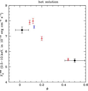
Fig. 6.— Evolution of the observed X-ray flux with phase, from the “hot”solution of the fits (see Table 4). The Chandra values are presented using black dots, the horizontal error bar corresponding to the phase span of the observations (Table 1); the four XMM-Newton datasets from 2005 are shown with open red triangles and that from 2008 with a blue cross. The agreement between both observatories is remarkable, considering the remaining differences in instrumental calibrations. It demonstrates the repetitive behavior of HD 191612 at high energies.
fits which are shown in the table. These fits were per-formed assuming the solar abundance of Asplund et al. (2009), which is why we also provide new fits for the XMM-Newton spectra previously presented in Naz´e et al. (2007, 2014). HD 191612, as other Of?p stars, ap-pears slightly enriched in nitrogen and depleted in car-bon and oxygen (Martins et al. 2015). However, con-sidering non-solar abundances (either by fixing them to the Martins et al. values or letting them vary freely) does not significantly improve the quality of the fits, nor does it change the conclusions, so we kept them solar.
The new Chandra data confirm the results derived previously on XMM-Newton observations: the flux of HD 191612 increase by ∼40% at maximum emission phase, and the X-ray emission appears harder when brighter. This strong agreement (see also Fig. 6) demonstrates the great stability in the X-ray proper-ties of HD 191612 over a decade (i.e. 7 periods of HD 191612).
4.3. Direct comparison with model predictions
In order to make a direct comparison between the MHD model and observations, we developed a new spectral model for XSPEC. We note that the X-ray emission from the confined winds is thermal and due to the high plasma densities the non-equilibrium ion-ization effects can be neglected. We thus consider thermal plasma in collisional ionization equilibrium. The model reads in the DEM as provided by the 3D MHD simulations averaged over 1.5 Ms of simulation time (from 0.5 to 2.0 Ms) and over all azimuthal angles (Fig. 7). To calculate the theoretical spectrum associ-ated with it, we make use of the optically thin plasma model (apec) for each plasma temperature of the input DEM. As free parameter, the model scaling factor sc indicates whether the total amount of hot plasma as de-rived in the hydrodynamic simulations (emission mea-sure= 2.7 × 1056cm−3over log(T ) = 6 to 8) matches that required by observation. For example, a sc= 1 in-dicates a perfect correspondence, while sc < 1 or > 1 means that the MHD model correspondingly predicts higher or smaller amount of hot plasma than required by the data, respectively. Note that abundances of the hot plasma are additional possible free parameters of this model. Finally, our new XSPEC model is able to take into account the kinematic information provided from the 3D MHD simulations as well. Thus, it is able to model the realistic line profiles (more on that further below).
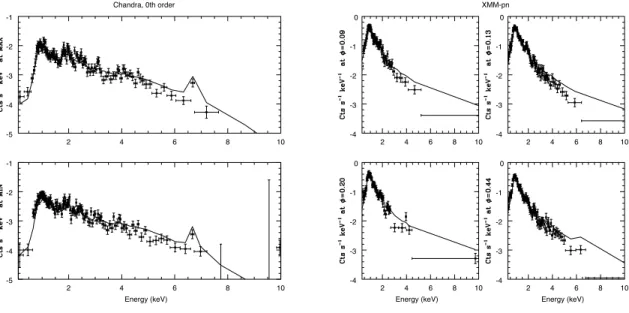
Chandra, 0th order 2 4 6 8 10 -5 -4 -3 -2 -1 2 4 6 8 10 -5 -4 -3 -2 -1 Energy (keV) XMM-pn 2 4 6 8 10 -4 -3 -2 -1 0 2 4 6 8 10 -4 -3 -2 -1 0 2 4 6 8 10 -4 -3 -2 -1 0 Energy (keV) 2 4 6 8 10 -4 -3 -2 -1 0 Energy (keV)
Fig. 8.— Comparison of the best-fit model using the simulated DEM (black line) with Chandra 0th order spectra (left, for maximum and minimum emission phases) and with XMM-Newton-EPIC pn spectra (right, for four different phases). Note the good fit up to 2–4 keV, and the slight excess of hard flux at larger energies.
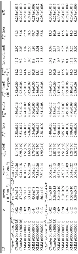
T able 4: Best-fit spectral parameters for a model of the type wab s × phab s × P 2 a1 pec . The columns F unab s X pro vide flux es corrected for the interstellar absorbing column (3 .2 × 10 21 cm − 2) only , while F int X yield the flux es corrected for the full absorbing columns The hardness ratios H R are defined as F unab s X (hard) /F unab s X (soft), with “tot”, “soft”, and “hard” corresponding to the 0.5–10. k eV , 0.5–2. k eV , and 2.–10. k eV ener gy bands, respecti v ely . The 1 σ errors were calculated in XSPEC using the err or command for parameters and the flux err command for observ ed flux es (the errors on H R s were calculated assuming the relati v e errors on observ ed and absorption-corrected flux es are equal). If asymmetric errors were found, the lar gest v alue is sho wn here. ID φ nor m1 nor m2 χ 2 red (dof) F ob s X (tot) F ob s X (soft) F ob s X (hard) F unab s X (tot, soft,hard) F int X (tot) H R (10 − 4cm − 5) (10 − 4cm − 5) (10 − 13 er g cm − 2s − 1) “W arm” solution: N ad d H = 5 × 10 21 cm − 2, k T = 0.24 and 1.8 keV Chandr a 0th (200975) 0.02 54.0 ± 3.2 7.66 ± 0.26 1.14(140) 7.38 ± 0.19 4.56 ± 0.16 2.82 ± 0.09 14.2 11.2 2.97 61.3 0.265 ± 0.013 Chandr a 0th (200976) 0.50 47.2 ± 2.6 5.21 ± 0.18 0.98(149) 5.53 ± 0.17 3.61 ± 0.12 1.92 ± 0.06 11.2 9.2 2.03 51.6 0.221 ± 0.010 XMM (0300600201) 0.09 55.9 ± 1.5 8.01 ± 0.23 1.51(169) 7.66 ± 0.13 4.74 ± 0.09 2.92 ± 0.11 14.6 11.6 3.07 62.9 0.265 ± 0.011 XMM (0300600301) 0.20 53.1 ± 1.2 6.63 ± 0.20 1.66(168) 6.68 ± 0.12 4.25 ± 0.06 2.42 ± 0.09 13.1 10.6 2.55 58.5 0.241 ± 0.010 XMM (0300600401) 0.44 45.9 ± 7.8 5.03 ± 0.11 1.76(236) 5.34 ± 0.06 3.50 ± 0.05 1.84 ± 0.06 10.8 8.9 1.93 49.7 0.217 ± 0.008 XMM (0300600501) 0.12 60.0 ± 1.5 7.85 ± 0.26 1.91(150) 7.76 ± 0.14 4.89 ± 0.06 2.86 ± 0.13 15.1 12.1 3.01 66.6 0.249 ± 0.012 XMM (0500680201) 0.13 56.4 ± 1.0 7.50 ± 0.14 1.90(241) 7.38 ± 0.09 4.64 ± 0.08 2.73 ± 0.08 14.3 11.5 2.88 62.8 0.250 ± 0.008 “Hot” solution: N ad d H = 0 , k T = 0.75 and 2.4 keV Chandr a 0th (200975) 0.02 3.14 ± 0.19 5.06 ± 0.21 1.12(140) 7.40 ± 0.20 4.46 ± 0.12 2.94 ± 0.10 13.3 10.2 3.09 13.3 0.303 ± 0.013 Chandr a 0th (200975) 0.50 2.56 ± 0.15 3.43 ± 0.15 1.05(149) 5.41 ± 0.12 3.38 ± 0.11 2.03 ± 0.09 10.0 7.8 2.13 10.0 0.273 ± 0.015 XMM (0300600201) 0.09 3.24 ± 0.10 5.52 ± 0.20 1.41(169) 7.90 ± 0.14 4.72 ± 0.10 3.17 ± 0.11 14.1 10.8 3.33 14.1 0.308 ± 0.013 XMM (0300600301) 0.20 3.10 ± 0.09 4.50 ± 0.17 1.51(168) 6.85 ± 0.13 4.23 ± 0.07 2.62 ± 0.10 12.5 9.7 2.75 12.5 0.284 ± 0.012 XMM (0300600401) 0.44 2.71 ± 0.05 3.37 ± 0.09 1.66(236) 5.48 ± 0.08 3.49 ± 0.05 1.99 ± 0.06 10.2 8.1 2.09 10.2 0.258 ± 0.009 XMM (0300600501) 0.12 3.53 ± 0.10 5.34 ± 0.22 1.28(150) 7.99 ± 0.17 4.90 ± 0.09 3.10 ± 0.13 14.5 11.2 3.25 14.5 0.290 ± 0.013 XMM (0500680201) 0.13 3.39 ± 0.68 5.04 ± 0.12 1.38(241) 7.60 ± 0.09 4.67 ± 0.06 2.93 ± 0.08 13.8 10.7 3.07 13.8 0.287 ± 0.009 Simulated DEM -1 -0.5 0 0.5 1 0 0.2 0.4 0.6 0.8 1 log(Energy in keV)
Fig. 7.— The time-averaged DEM per log(E)= 0.1 (in keV) as derived from 3D MHD simulation, normalized to its peak. The total E M= 2.7 × 1056cm−3when in-tegrated over log(T ) =6 to 8, is comparable to what was found in simulations of θ1Ori C (∼ 9 × 1055cm−3 integrated over the same temperature range) though it is somewhat larger as it corresponds to a larger mag-netosphere.
6.14 6.16 6.18 6.2 6.22 6.24 0.01 0.02 0.03 Pole-on Equator-on no broad. Gaussian broad. 6.14 6.16 6.18 6.2 6.22 6.24 0.005 0.01 0.015 Pole-on Equator-on no broad. Gaussian broad.
Fig. 9.— The Si xiv Lymanα line profile observed in unbinned MEG spectra at maximum (top) and mini-mum (bottom) emission phases, compared to results of different fits (see Table 6): simulated DEM without broadening (green dashed line), with Gaussian broad-ening (blue long-dashed line), or with the line profile found in simulations (either for a pole-on situation, black solid line, or an equatorial view, dotted red line).
We began by fitting this model to the low-resolution spectra (both 0th order Chandra and XMM-Newton spectra). First, we allowed the possibility of ab-sorption in addition to the interstellar column (3.2 × 1021cm−2, see above), but this results in a 1σ upper limit on Nadd
H of 2 × 10
19cm−2, indicating that the in-terstellar absorption is sufficient to fit the spectra. We therefore consider only the (fixed) interstellar absorb-ing column in what follows. The results of the fits are provided in Table 5 and shown in Fig. 8. Again, a very good agreement is found between XMM-Newton and Chandra results. The spectra appear very well fitted up to 3 keV, but the model slightly overpredicts the flux at higher energies. This is reflected in the hard-enss ratio HR, which is about 0.45 (fixed value, since the DEM shape is fixed) when simpler fits favor values of ∼0.25–0.3 (Table 4). This can be explained by the presence of plasma at high temperatures in the MHD model (see previous sections, in particular Fig. 2).
The scaling factors also indicate an overprediction of the X-ray output by a factor ∼ 5. The added third dimension is a bit less efficient than 2D, but one other suggestion to explain this difference is the cho-sen value of the mass-loss rate. Indeed, considering the dense wind of HD 191612, cooling should be ef-ficient, hence LX ∼ ˙M−2, and it is known that mass-loss rates of massive stars are overestimated by a fac-tor ∼ 3 because of clumping within the stellar wind (e.g. Bouret et al. 2005). In addition, such a reduction of mass loss rate would lead to an effect called ‘shock retreat’ (ud-Doula et al. 2014), wherein shocked gas retreats towards the stellar surface along the field lines where the velocities are lower, leading to lower shock speeds hence possibly to softer X-rays - though the effect needs to be quantified exactly for a star like HD 191612. However, we should keep in mind that even the dynamical model presented here has its own shortcomings, e.g. it only uses the radial component of the radiative force and it ignores cooling due to inverse Compton scattering which, although having a relatively minor effect for O stars (ud-Doula et al. 2014), does slightly reduce the amount of hard X-rays. Future models should indeed address these shortcom-ings.
As the simulated DEM is an average value, it is not made to reproduce the flux variations recorded for HD 191612. Such variations are usually considered to be due to occultation of the hot plasma by the stellar body, when confined winds are seen edge-on. How-ever, such a simple occultation cannot match the
ob-served decrease in flux considering the hot plasma lo-cation (about 1.6–2.8 R∗ for HD 191612, see previous sections): at this position, occultation effects would lead to flux changes of about 15%. To get the observed 40% would require an improbably close location for the confined winds (r < 1.2R∗, see ud-Doula & Naz´e 2016). Therefore, an additional mechanism is needed. A plausible scenario is the presence of asymmetries in the confined wind structure, which would enhance occultation effects. They could be linked e.g. to an off-center magnetic dipole or to multipolar components to the magnetic field. Current spectropolarimetric ob-servations only sample the dipolar component of the magnetic field, yielding no constraint yet on such fea-tures. More precise knowledge of the magnetic ge-ometry, and its consequences on the wind confinement through a new modeling, is thus needed before the in-creased flux variability can be understood.
As a second step, we fitted the Chandra high-resolution spectra, allowing for non-solar abundance in the elements whose lines are clearly seen in the HEG/MEG spectra (i.e., Ne, Mg, Si, S, Fe). Note that, for this exercise, the high-resolution spectra were binned in a similar way as the lower-resolution ones (see end of §2). Furthermore, to avoid the UV-depopulating effects modifying the f /i ratios which are not considered in apec, the f and i lines of He-like triplets were grouped in a single bin. As the instrumen-tal broadening of HEG/MEG spectra is much smaller than for low-resolution data, an intrinsic broadening can be more easily detected. Therefore, we tested several hypotheses: (1) no intrinsic broadening, (2) Gaussian broadening (whose amplitude was let free to vary), and (3) simulated line profiles (Fig. 3). The latter scenario allows us to perform a fully coherent comparison between data and 3D MHD simulations, as it uses the complete physical picture (simulated dis-tribution of emissivity as a function of temperature and velocity) provided by the model.
Results of these fits are provided in Table 5 and shown for the best lines in Fig. 9. The scaling factors are similar to those found on lower-resolution spectra (indeed, a global fit to all Chandra spectra also yields similar results). Derived abundances are quasi solar: indeed, the solar abundance is within 1–2σ of the fitted value for Ne, Mg, Si, and S or within 3σ for Fe. Be-sides, letting them freely vary only allows to (slightly) improve the χ2 (e.g. from 0.36 to 0.29 for the Gaus-sian broadening case). The fitting results thus show no clear and definitive evidence for non-solar abundances
for these elements. A comparison between the di ffer-ent broadening hypotheses is more interesting. Even if the differences are marginal, note that the worst χ2is obtained for no broadening, and the best one for Gaus-sian broadening. The FWHMs in this case are twice smaller than found on individual line analysis (but this remains within the errors, see Sect. 4.1) and, as in that analysis, the derived Gaussian broadening is again slightly larger at minimum emission phase, though the difference is marginal (within 2σ). The best-fit Gaus-sian broadening has a larger value than measured in the simulated profiles (see end of §. 4.1 and Fig. 4). This certainly indicates that the observed X-ray lines are broader than expected, as already derived from the line-by-line analysis. Yet, the very good agreement be-tween observations and model predictions and the very limited improvement when considering a larger broad-ening are remarkable, showing that only further refine-ments of the model are still needed.
5. Conclusion
We have obtained Chandra data of the magnetic Of?p star HD 191612 at two crucial phases (maximum and minimum emissions, when confined winds are seen face-on and edge-on, respectively). These new data show great similarities with XMM-Newton-EPIC spectra (i.e. 40% flux decrease and spectrum softening at minimum), demonstrating the quasi-perfect repeata-bility of the X-ray behavior over a decade. The high-resolution data further reveal more detail, with many similarities with HD 148937 and θ1Ori C, the only two other magnetic O-stars observed at high-resolution: small (but non-zero) line broadenings for high-Z el-ements, negligible line shifts, hot plasma located at a few stellar radii from the star. In addition, compar-ing spectra of HD 191612 at the two phases yields no significant change except for flux - the slightly larger broadening and slightly lower line shift found at min-imum phase are only marginal, 1σ changes, thus re-quiring confirmation with future X-ray facilities such as Athena-XIFU.
We further compared the observational results with predictions from a dedicated 3D MHD simulation of confined winds in HD 191612. To this aim the sim-ulated DEM was directly fitted to the observed spec-tra. The low-resolution data appear well fitted up to ∼3 keV, a slight overprediction is seen at higher en-ergies which can possibly be mitigated by including inverse Compton cooling in future models. At
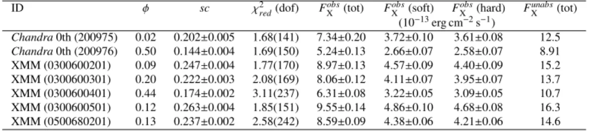
high-Table 5: Best-fit parameters for the dedicated confined wind model for low-resolution spectra.
ID φ sc χ2red(dof) FobsX (tot) FobsX (soft) FobsX (hard) FunabsX (tot)
(10−13erg cm−2s−1) Chandra0th (200975) 0.02 0.202±0.005 1.68(141) 7.34±0.20 3.72±0.10 3.61±0.08 12.5 Chandra0th (200976) 0.50 0.144±0.004 1.69(150) 5.24±0.13 2.66±0.07 2.58±0.07 8.91 XMM (0300600201) 0.09 0.247±0.004 1.77(170) 8.97±0.13 4.57±0.09 4.40±0.09 15.2 XMM (0300600301) 0.20 0.222±0.003 2.08(169) 8.06±0.12 4.11±0.07 3.95±0.07 13.7 XMM (0300600401) 0.44 0.174±0.002 3.11(237) 6.31±0.08 3.22±0.05 3.09±0.05 10.7 XMM (0300600501) 0.12 0.263±0.004 1.85(151) 9.55±0.14 4.86±0.10 4.68±0.08 16.3 XMM (0500680201) 0.13 0.237±0.002 2.58(242) 8.59±0.09 4.38±0.06 4.21±0.06 14.6
Table 6: Best-fit parameters for the dedicated confined wind model for high-resolution Chandra spectra. Abundances are in number, relative to Hydrogen and with respect to solar abundance ratios
.
Model sc(MAX) sc(MIN) χ2
red(dof) a Ne Mg Si S Fe Funabs X (tot, MIN–MAX) (10−13erg cm−2s−1) no broadening 0.280±0.017 0.176±0.011 0.37(500) 1.37±0.33 0.71±0.08 1.12±0.10 1.30±0.46 0.60±0.14 15.5–9.79 Gaussian broad.b 0.260±0.015 0.164±0.011 0.29(498) 2.20±0.54 1.22±0.19 1.50±0.15 1.50±0.50 0.69±0.16 15.4–9.81 Pole-on model 0.275±0.017 0.173±0.011 0.33(500) 1.50±0.36 0.84±0.10 1.24±0.11 1.37±0.48 0.63±0.14 15.4–9.71 Equ.-on model 0.279±0.017 0.175±0.012 0.33(500) 1.56±0.37 0.85±0.10 1.26±0.12 1.37±0.48 0.64±0.15 15.4–9.69
aChandradata of maximum and minimum phases were fitted simultaneously, allowing for different scaling factors but forcing abundances to be the
same: a single χ2is thus provided for both phases.
b
For the gaussian broadening (gsmooth model within XSPEC), the FWHMs were found to be 248±45 km s−1and 306±58 km s−1for maximum and minimum emission phases, respectively.
resolution, the X-rays lines also appear quite well fit-ted by the model, though a larger broadening yields slightly better results. A scaling of the total predicted flux by a factor of ∼5 is needed but this can be ad-dressed by some reduction of the mass-loss rates, prob-ably due to clumping of the wind.
Refinements in the modeling are certainly needed, but the remarkable agreement between data and model certainly shows that the basic picture is promising. One avenue to investigate may be linked to asymme-tries. Indeed, occultation of an axisymmetric equato-rial structure located at the position of the X-ray emit-ting plasma cannot explain the observed flux variation of 40%, while an asymmetric distribution, linked e.g. to a magnetic geometry more complicated than a sim-ple centered dipole, may well do so.
YN acknowledges support from the Fonds National de la Recherche Scientifique (Belgium), the Commu-naut´e Franc¸aise de Belgique, the XMM PRODEX contract (Belspo), and an ARC grant for concerted research actions financed by the French community of Belgium (Wallonia-Brussels federation). AuD acknowledges support by NASA through Chandra Award numbers GO5-16005X, AR6-17002C and G06-17007B issued by the Chandra X-ray Observatory
Center which is operated by the Smithsonian Astro-physical Observatory for and behalf of NASA under contract NAS8-03060. ADS and CDS were used for preparing this document.
REFERENCES
Asplund, M., Grevesse, N., Sauval, A. J., & Scott, P. 2009, ARA&A, 47, 481
Babel, J., & Montmerle, T. 1997a, A&A, 323, 121
Bouret, J.-C., Lanz, T., & Hillier, D. J. 2005, A&A, 438, 301
Castor, J. I., Abbott, D. C., & Klein, R. I. 1975, ApJ, 195, 157
Donati, J.-F., Howarth, I. D., Bouret, J.-C., et al. 2006, MNRAS, 365, L6
Fossati, L., Castro, N., Sch¨oller, M., et al. 2015, A&A, 582, A45
Gagn´e, M., Oksala, M. E., Cohen, D. H., et al. 2005, ApJ, 628, 986 (erratum in ApJ, 634, 712)
Howarth, I. D., Walborn, N. R., Lennon, D. J., et al. 2007, MNRAS, 381, 433
Koen, C., & Eyer, L. 2002, MNRAS, 331, 45
MacDonald, J., & Bailey, M. E. 1981, MNRAS, 197, 995
Marcolino, W. L. F., Bouret, J.-C., Sundqvist, J. O., et al. 2013, MNRAS, 431, 2253
Martins, F., Herv´e, A., Bouret, J.-C., et al. 2015, A&A, 575, A34
Naz´e, Y., Vreux, J.-M., & Rauw, G. 2001, A&A, 372, 195
Naz´e, Y. 2004, Ph.D. Thesis, University of Li`ege
Naz´e, Y., Barbieri, C., Segafredo, A., Rauw, G., & De Becker, M. 2006, Information Bulletin on Variable Stars, 5693, 1
Naz´e, Y., Rauw, G., Pollock, A. M. T., Walborn, N. R., & Howarth, I. D. 2007, MNRAS, 375, 145
Naz´e, Y., ud-Doula, A., Spano, M., et al. 2010, A&A, 520, A59
Naz´e, Y., Zhekov, S. A., & Walborn, N. R. 2012, ApJ, 746, 142
Naz´e, Y., Petit, V., Rinbrand, M., et al. 2014, ApJS, 215, 10 (erratum 2006, ApJS, 224, 13)
Naz´e, Y., Wade, G. A., & Petit, V. 2014, A&A, 569, A70
Naz´e, Y., Sundqvist, J. O., Fullerton, A. W., et al. 2015, MNRAS, 452, 2641
Petit, V., Cohen, D. H., Wade, G. A., et al. 2015, MN-RAS, 453, 3288
Schulz, N. S., Canizares, C., Huenemoerder, D., & Tibbets, K. 2003, ApJ, 595, 365
Sundqvist, J. O., ud-Doula, A., Owocki, S. P., et al. 2012, MNRAS, 423, L21
ud-Doula, A., & Owocki, S. P. 2002, ApJ, 576, 413
ud-Doula, A., Owocki, S. P., & Townsend, R. H. D. 2008, MNRAS, 385, 97
ud-Doula, A., Sundqvist, J. O., Owocki, S. P., Petit, V., & Townsend, R. H. D. 2013, MNRAS, 428, 2723
ud-Doula, A., Owocki, S., Townsend, R., Petit, V., & Cohen, D. 2014, MNRAS, 441, 3600
ud-Doula, A., & Naz´e, Y. 2016, Advances in Space Research, 58, 680
Wade, G. A., Howarth, I. D., Townsend, R. H. D., et al. 2011, MNRAS, 416, 3160
Wade, G. A., Neiner, C., Alecian, E., et al. 2016, MN-RAS, 456, 2
Walborn, N. R. 1973, AJ, 78, 1067
Walborn, N. R., Howarth, I. D., Herrero, A., & Lennon, D. J. 2003, ApJ, 588, 1025
Walborn, N. R., Howarth, I. D., Rauw, G., et al. 2004, ApJ, 617, L61
This 2-column preprint was prepared with the AAS LATEX macros