Computer model of a nuclear reactor primary coolant pump

COMPUTER MODEL OF A NUCLEAR REACTOR PRIMARY COOLANT PUMP

by

KEAN WONG

B.S., Cornell University

(1980)

Submitted to the Department of Nuclear Engineering

in Partial Fulfillment of the Requirements of the Degree of

MASTER OF SCIENCE IN NUCLEAR ENGINEERING at the

MASSACHUSETTS INSTITUTE OF TECHNOLOGY

August, 1982

@

Signature of Author

Certified by

Accepted by

Department

f

U

Allan F. Henry Chairman, Departmental Graduate Committee

Archives

MASSACHUSETTS INSTITUTE OF TECHNOLOGY

'AN 181 7

I

COMPUTER MODEL OF A NUCLEAR REACTOR PRIMARY COOLANT PUMP

by

KEAN WONG

Submitted to the Department of Nuclear Engineering in August, 1982 in partial fulfillment of the requirements for the Degree of Master of Science in

Nuclear Engineering

ABSTRACT

The performance of a reactor coolant pump should be modeled accurately so that it made be used in a reactor plant

computer to provide information for the operator.

This study develops techniques to represent the gross performance of a coolant pump. Dimensionless quantities are used to describe the characteristic curves of a pump.

Also, in order to calculate flow transients, the hydraulic characteristics of the various flow paths are also modeled.

To test these models,a computer program is used to incorporate the pump model and the flow model to predict the reactor vessel flow during transients. Two specific applications of the computer.program are shown at the end of the report.

Thesis Supervisor: John E. Meyer

ACKNOWLEDGEMENTS

The author is indebted to Prof. John E. Meyer, who as thesis adviser gave much assistance, encouragement, and guidance. I would also like to thank Paul Bergeron and Ken Rousseau of Yankee Atomic Electric Company, for information concerning the Maine Yankee Reactor during flow coastdown. The information in this thesis cited as deriving from "Maine Yankee", however, should not be considered as representing

that actual system in its current or projected operating configuration, but as an idealization thereof. In particular, the results so identified in this report have not been either reviewed or approved by the Yankee organization. Final thanks are to Charles Stark Draper Laboratory for providing funds for the computer work.

TABLE OF CONTENTS Page TITLE PAGE 1 ABSTRACT 2 ACKNOWLEDGEMENTS 3 TABLE OF CONTENTS 1.INTRODUCTION 7 2.PUMP BEHAVIOR 8 2.1.General Description 8 2.2.Dimensional Analysis 9 2.3.Head-Capacity Curve 10

2.4.Brake Horsepower Curve and Motor Torques 12 2.5.Net Positive Suction Head Curve 19

2.6.Mechanical Seals 19

3.LOOP FLOW BEHAVIOR 24

3.1.Mass Flow Equation and Resistances 24

4.COMPUTATIONAL METHOD 28

4.1.Finite Difference Equations 28

5.SENSOR FAILURE DETECTION AND IDENTIFICATION 29

5.1.Idealized Cases 29

5.2.Actual Cases 30

6.APPLICATIONS

6.1.Example from Fuls' Report ₃₃

6.1.1.Rated Conditions 37

6.1.2.Flow Geometries ,

6.1.3.Head-Capacity Curve ₃₄

6.1.4.Brake Horsepower Torque 36

6.1.5.Mass Flow Equation ₃₇

6.1.6.Pump Speed Equation 39

6.1.7.Calculations ₄₀

6.1.8.Conclusions ₄₀

6.2.Maine Yankee Reactor 43

6.2.1.Maine Yankee Head-Capacity Curve 43 6.2.2.Maine Yankee Brake Horsepower Curve 47

6.2.3.Maine Yankee Net Positive Suction Head Curve 51

6.2.4.Mass Flow Equation 54

6.2.5.Pump Speed Equation 63

6.2.6.One Pump Failure Transient ₆₄

6.2.7.Complete Loss-of-Flow Accident 68

6.2.8.Conclusions ₇₁

7.CONCLUSIONS AND RECOMMENDATIONS 72

APPENDIX A: COMPUTER PROGRAM USED FOR THE

EXAMPLE FROM FULS' REPORT ₇₃

A.1.Nomenclature ₇₃

A.2.Program Listing ₇₄

APPENDIX B: COMPUTER PROGRAM USED FOR

MAINE YANKEE REACTOR 78

B.1.Nomenclature ₇₈

B.2.Program Listing 79

1.INTRODUCTION

This study develops techniques to represent the gross performance of a coolant pump. Many existing works on pumps do not give detailed information on how the pump can be modeled. Valid pump models can be used in many ways to predict flow values during a plant flow transient.

One of these ways is to use the model on a plant computer. Computed output can supplement sensor measurements and provide better information for the operator(e.g. in the manner of Ray(1)).

To represent the performance of a pump, dimensionless quantities are used to describe characteristic curves of the pump. These curves are the head-capacity curve, the brake horsepower curve, and the net positive suction head curve. An equation that represents each curve is developed for one

or more typical cases.

There is one more group of features that must be modeled in order to calculate flow transients. The hydraulic characteristics (friction, shock, and inertia) of the various flow paths must be described.

To test these models, a computer program is used to incorporate the pump model and the flow model to predict the mass flow through the reactor during transients. The transient considered is loss of power to the pump motor with a consequent loss of coolant flow through the core. Two specific applications of the computer program are shown at the end of the report(Chapter 6).

2.PUMP BEHAVIOR

2.1.General Description

A nuclear reactor primary coolant pump provides the means for _{forced circulation of coolant. In this case, the} pump is connected to the primary loop of a pressurized water reactor (PWR). _{The water coolant is transferred from the} reactor core to the steam generator and returned.

The pump's main components are an electric motor, a pump impeller, and a mechanical seals region. The electric motor is located at the top of the pump. Electrical current is supplied to the motor at high voltage and three phases. The motor converts this electrical power into the rotation of the pump impeller. The _{impeller rotation causes coolant flow} through the coolant loop and a pressure rise across the pump. The mechanical _{power associated with the impeller} rotation _{is described by the brake horsepower (BHP) curve.} The BHP curve describes the amount of torque and consequently the power needed to keep the impeller rotating at a specified speed. The power (pressure drop/flow) imparted to the fluid is described by the head-capacity (h-c) curve. The h-c curve shows how much pressure _{drop and consequently the power} imparted to the fluid at a certain mass flow through the pump . _{The difference between the BHP and the h-c curve largely} represents losses in the fluid flow through the pump.

There are two requirements on the pump during normal operation. The first _{is that the pump must provide enough} pressure drop/flow to overcome all losses in one complete

9

trip around the loop. These losses are due to friction and

shock effects when the fluid moves through each component of

the loop.

The second requirement is that pump pressure

entering the pump impeller must never be less than the

fluid

vapor pressure.

If this occurs, some of the fluid will

vaporize in the pump

-

is called cavitation. Cavitation can

cause a decrease in the head supplied at a given flow and the

bubble collapse can cause damage to the pump

impeller.

2.2 .Dimensional

Analysis

There are only a few reports, Fuls(2) and Tong(3), that

describe in detail how to represent the performance of a

pump. Most reports, Burgreen(4) and Boyd(5), describe the

performance of the pump using affinity laws but they do not

give much detail about the derivation of these laws.

The main reference used in this section is the report by

Fuls(2).

In his report he describes the use of dimensionless

quantities to represent the characteristic curves of the

pump. Three of these quantities are:

pw

P

T

=

where

(kg/m 3)

10

W = mass flow (kg/s) u = viscosity (Pa-s)

D = pump impeller diameter (m)

&p = pressure rise through the pump (densityxhead) (Pa)

w = pump speed (rad/s)

For this case the principles of dimensional analysis can be stated:

a)consider a class of pumps for which all geometrical features - lengths, radii, etc., - are scaled to be directly proportional to the impeller diameter;

b)for these pumps assume that only the quantities listed after equation 2.2a need be specified to completely define pump operation; and

c)if this assumption is valid, then for its range of validity and for all the pumps in this class,

TT

unique function of TT1 and 7 .

This is a very useful result and gives the so called affinity laws, Fuls(2), of pump performance. Furthermore for many fluids (excluding tars, etc.) the effect of variation in

(Reynolds number)-T₁lis unimportant. This is a good approximation for liquid water and is adopted.

2.3.Head - Capacity Curve

To represent the head-capacity curve we use the two remaining dimensionless quantities (after dropping Reynolds number dependence):

11

w

e1p = pressure rise through the pump D = pump impeller diameter

S= density

(Note - when we talk about head-flow we mean pressure rise-flow)

An additional simplification is employed when we consider the operation of many states of a single pump (one pump diameter). Consider one of these states to be a "rated condition" (subscript R). Also note that multipling each -7 quantity by a constant does not change the dimensional analysis conclusions.

Therefore dividing TT772 by TT2R and 773 by TT3R

where R is _{the rated value of the mass flow, density, pump} speed, and pressure rise, we arrive at:

-T 2R =

2

T WRD

3R =R

R

12

The resulting variables are Y and x, where:

-73

Y

-P TT3R

TT2R

The relationship betwee

(,p)(R) (WR)

(W)( R)(R)

(WR)(

)(w)

Y and x is

Y = g(x)

where g(x) is determined by the given head-capacity (obtained by a pump test).

(2.3c)

curve

2.4.Brake Horsepower Curve and Motor Torques

To represent the brake horsepower (BHP) curve, we developed a dimensionless quantity not mentioned in Fuls'(2) report. This term is:

P

75

where

P = power input to the pump(commonly called brake horsepower)(W)

= density w = pump speed

D = pump impeller diameter

(2.3a)

(Note: when we talk about brake horsepower we use Watts to represent it).

Power divided by pump speed is equal to torque. Therefore T75 is equivalent to:

Tb (2.4b)

I75

2

(2.4b)

where

T_b = brake horsepower torque (N m)

We divideF 5 by its rated valuerr5R which is: TbR S75R 2 5 RWRD 2 7 ₅ (Tb )(WR) 2 ?R ) Y (2 .4cr) Ts5R (TbR)(w)2 )

YT is again considered to be a function of only one variable -x- where x is defined by equation (2.3b).

The relationship between YT and x is:

YT = f(x) (2.4d)

where f(x) is defined by the given BHP curve.

The brake horsepower is also used to calculate the pump efficiency. Pump efficiency describes how much of the mechanical power associated with impeller rotation (BHP) is actually imparted to the fluid. To determine pump

efficiency, first convert the value of pressure rise through the pump to power. We multiply pressure rise by the fluid mass flow through the pump and also divide by the fluid

density. This gives the power imparted to the fluid and we divide this value by the BHP value(at that mass flow) to obtain the pump efficiency at a given mass flow.

Equations (2.4a)-(2.4d) provide information on obtaining Tb (brake horsepower torque). This is the torque requirement

to cause the impeller shaft to move the current value of mass flow rate with the current pump pressure rise. Two other torques act on the rotating parts; Te - electric torque provided by the electric motor; and Tw - windage and bearing

loss torque.

The electric torque for a 3 phase induction motor is depicted in figure 2.4.1. This figure show how the electric

torque varies with pump impeller speed; from start speed to rated speed.

From Smith(6), the equation for rated electric torque for a 3 phase induction motor is:

2

T _eR - (2.4e)

swS

where

12 = electric current in rotor R2 = resistance of rotor

w = synchronous pump speed s = slip = w - w

wS

When electrical power is turned off or lost to an induction motor, magnetic flux is trapped in the rotor. As the rotor continues to turn, the trapped flux generates

Rated Pump Impeller Speed 2. 1. Electric 1. Torque (T/Tf 0. 0.0 0.5 1.0

Pump Impeller Speed

1 (w/wR) C I

I

-

-I

-.00

Figure 2.4.1 Electric Torque vs. Pump Impeller Speed (ref.-Smith( 6))

Rated Electric Torque

currents in the stator. The induced stator currents(called eddy currents) produces a retardation torque on the rotor. Therefore the rotor begins to slow down and the electric torque decays. The formula for the electric torque for loss of electric current to the pump motor, from Boyd(5), is:

S= T e(e-t/tau) 2(w) (2.4f) e eR

(w_R where

t = time (s)

tau = time decay constant of electric torque (s) From Fuls'(2) report, the electric torque is assumed to go instantaneously to zero. Therefore the value of tau is very small. _{I have also made this assumption and have used} tau equal to 10- / _{second for the examples in Chapter 6.}

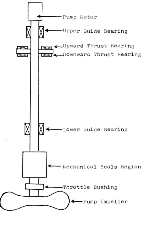
The windage and bearing loss torque are due to the bearings limiting the motion of the pump shaft. There are an upper and a lower guide bearing which limits radial shaft motion and an upward and a downward thrust bearing which limits axial shaft motion. The location of the bearings is shown in figure 2.4.2. From Fuls(2), the formula for windage and bearing loss torque is:

Tw = Tw R(W/wR)2 w>.19wR (2.4g) = .03 5TwR _O<w<.19

wR

= .1TwR w = 0

TwR = rated windage and bearing loss torque (N-m).

The torque equation describes how the pump speed varies with the electric torque, the brake horsepower torque, and the windage and bearing loss torque.

I dw = Te - Tw - Tb (2.4h)

dt

I = moment of inertia of rotating parts (kg.m w = pump speed

t = time

Te = electric torque (N.m)

T_b = brake horsepower torque (N m) T _w = windage and bearing torque (N m)

Pump iiotor

---- Upper Guide Bearing

*.-Upward Thrust Bearing : ownward Thrust Bearing

--- Lower Guide Bearing

.--i.echanical Seals Region

e Bushing

--- Pump Impeller

Figure 2.4.2 Location of Bearings (ref.-Maine Yankee(7))

2.5.Net Positive Suction Head Curve

To represent the net positive suction head (NPSH) curve, we again use Y pdefined by equation (2.3a) but /p is the pressure difference between the pressure at the suction nozzle and the fluid vapor pressure. Y p, again is only a

function of one varible -x- defined by equation (2.3b). The relationship between Y p,and x is:

Y ,= h(x) (2.5a)

where h(x) is defined by the given NPSH curve.

2.6.Mechanical Seals

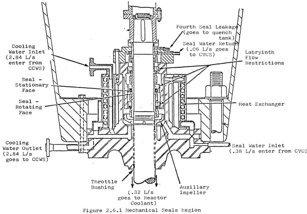
The purpose of the mechanical seals is to limit the leakage of reactor coolant along the impeller shaft to the surroundings. Each seal consists of two highly polished surfaces, positioned in parallel, one surface attached to the rotating shaft and the other surface attached to a stationary portion of the pump. Surrounding the seals is a heat exchanger which cools the seals, an auxillary impeller, a throttle bushing, and piping that sends to and removes from the seals water that acts as a coolant and lubricant for the surfaces.

There are many varieties, Karassik(8), of seal configurations. One arrangement that is used in Maine Yankee pumps(7) is now discussed for illustrative purposes. There are four mechanical face seals in each Maine Yankee pump. Three of the seals are mounted in a cartridge and they are

used to contain the reactor coolant pressure. The fourth seal is mounted on top of the cartridge.

Roughly 2.84 liters per second (L/s) from the component cooling water system (CCWS) and 0.38 L/s from the chemical and control volume system (CVCS) enter the mechanical seal area. 2.84 L/s goes to the heat exchanger and 0.32 L/s is pushed through the throttle bushing by the auxillary impeller and goes to the reactor coolant. 0.06 L/s is sent to the seals.

The 0.06 L/s sent to the seals passes through labryinth flow restrictions which bypass each of the three mechanical seals in the cartridge. The labryinth flow restrictions are designed to divide the total pressure drop across the first three seals so that each seal has the same pressure differential. The flow past the third seal region is piped back to the CVCS. Any leakage past the fourth seal is sent to the quench tank. The seals region and the flow through the region are shown in figures 2.6.1 and 2.6.2.

There are sensors that measure the pressure of the seal water after passing through the three seals in the cartridge. There is also a sensor that measures the pressure difference across the throttle bushing. If for example one of the seals fails, this will cause an increase in the seal water return flow to the CVCS. An increase in the return flow will cause a decrease in flow rate and pressure drop across the throttle bushing. An operator seeing the decrease in pressure drop across the throttle bushing will increase the flow from the

21

CVCS into the seal area to restore the pressure drop and flow

Cooling Water Inlet (2.84 L/s enter from

ccws)

SSeal Water Inlet

(.38 L/s enter from CVCS)

Bushing T v Auxi llary

(.32 L/s Impeller

goes to Reactor Coolant)

Figure 2.6.1 Mechanical Seals Region (ref-Maine Yankee(7))

Seal -Stationary. Face Seal -Rotating Face

Seal Water Flow

to Third Seal

Figure 2.6.2 General Diagram of

Second Mechanical Seal

24

3.LOOP FLOW BEHAVIOR

The pump is only a part of the operating description for the reactor coolant system(RCS). We must also describe the resistances to flow when the coolant moves through the various RCS components.

To describe the loop flow, two equations are used. The first equation deals with how the pump impeller speed changes with the torques applied within the pump, equation (2.4h). This equation is important because the performance of one of the RCS components - pump - is dependent on the pump speed.

The second equation relates changes in loop mass flow to pressure losses across each RCS components. In this equation we have assumed the fluid density remains constant even during transients. Therefore, for the case of flow coastdown, the result will be no occurence of natural

circulation.

During some loop flow transients, the flow many reverse in a loop and the mass flow equation takes this into consideration. When the flow does reverse in a loop, the pump impeller in that loop does not reverse its rotation. The pump has an anti-reverse rotation device to prevent impeller reverse rotation. In this situation, the pump does not deliver a pressure rise to the fluid but acts as a resistance to flow and causes a pressure loss.

3.1.Mass Flow Equation and Resistances

25

components is:

T- (L i) dWi (3 la)

i (Ai) dt itp

where

L.= ith component length (m)

A .- ith component cross sectional area (m 2) 1

W .= mass flow through ith component (kg/s)

t = time (s)

Ap

\,pP= pressure rise across the pump (Pa)

The formulas for friction and shock pressure drop are:

L(f l W) ( P)fr 2 (3.1b) and ( sh

Z

A = cross sectional area of flow (m2 )

D_h = hydraulic diameter (m)

f = friction pressure drop constant

Y = fluid density (kg/m3 )

26

Also, the reactor vessel has another pressure drop term. This is due to the spacers holding the fuel rods in the core. The spacer pressure drop formula is:

C 21wlw

(d),p =2 (3.id)

sp 2A29

C = modified drag coefficient

V

= ratio of projected grid cross section to undisturbed flow cross section

4 p is equal to the head capacity curve described in section(2.3). When the flow reverses in the loop the head-capacity curve is replaced with equation (3.1c). No information defining the value of K was found. It was arbitrarily set equal to -5 in all the examples in Chapter 6.

The different types of RCS components are the reactor vessel(composed of many hydraulic sub-components), the piping connecting the components, the reactor coolant pump, the stop valves, and the steam generator. There is a bypass stop valve directly connecting the two stop valves in the loop. This valve is also a RCS component but we have asssumed that

it is closed during all situations and the loop flow is through the other components.

The mass flow through the piping, the reactor coolant pump, the stop valves, and the steam generator is the same. Therefore, equation (3.1a) is:

(LRV RV i L p pi (3.1e)

(AD Rv Idt L__ (Ai) dt P4t'P

where V' i*RV itp

WRV= _{reactor vessel flow (kg/s)}

WL = loop flow (kg/s)

the first summation is taken over all components in the loop under consideration(but not the reactor vessel); and the second summation is taken over the same components and the reactor vessel.

The reactor vessel flow (WRV) is equal to the sum of the flows in all of the loop. Therefore, the flow in each loop is coupled to the flow in the other loops. If pump failure occurs in one loop, this will cause a smaller reactor vessel mass flow and a smaller pressure drop. A smaller reactor vessel pressure drop causes a smaller pressure rise delivered by the nonfailed pumps. Therefore, the flow in the loops with the nonfailed pumps will increase.

28

4.COMPUTATIONAL METHOD

4.1.Finite Difference Equations

Equations (2.4h) and (3.1a) can be cast into finite difference equations: /t j j-1 j-1 Aw= (T _e Tb _b - T _w ) (4.1a) 1 (L RV) - ₁

7-

(L

)

(ARV)

j

j

To calculate the present value or jth value of the change in pump impeller speed and the change in loop mass flow, we use the previous values or j-1 th values of the loop mass flow, the reactor vessel mass flow, and the torques.

There is a limitation imposed on these equations. The value of _{the time increment (/\t) must not be too large or} else the results become inaccurate. For the examples shown in Chapter 6, a At no greater than 0.1 second is used. Work was done on values of 0.2 and 0.5 seconds for

At.

5.SENSOR FAILURE DETECTION AND IDENTIFICATION 5.1.Idealized Cases

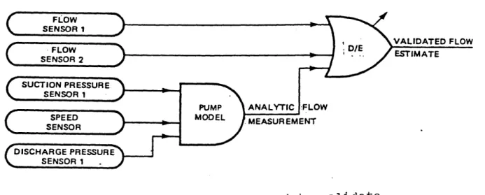
The pump model can be used to validate flow sensors. The simplest situation from Hopps( 9), is shown in figure

5.1.1.

The inputs to the pump model are sensors supplying a pump speed, a suction pressure, and a discharge pressure. In the pump model, the pressure head delivered by the pump is a function of the pump impeller speed and the mass flow through the pump. The difference between the discharge pressure and the suction pressure is equal to the pressure head. Once the pressure head and the pump speed are known, the mass flow can be determined. Two flow sensors are necessary in order to determine which flow value is correct if there is a discrepancy in flow values between one of the flow sensors and the pump model.

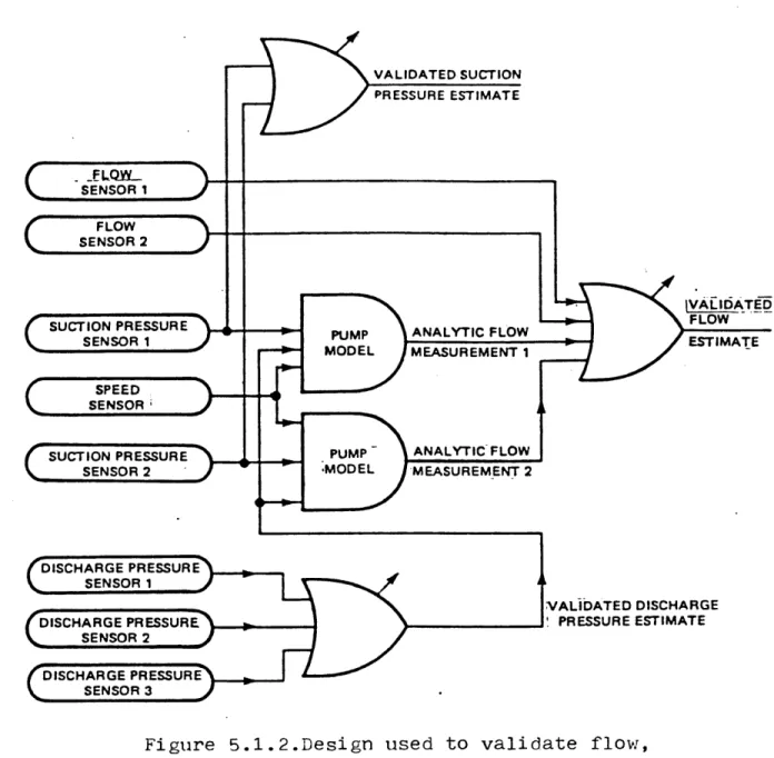
A more elaborate scheme, from Hopps(9 ), can be devised to test the other sensors besides the flow sensors. This design is shown in figure 5.1.2.

In this case, there are two pump models and redundancy in suction and discharge pressure sensors. Both the suction and discharge pressure sensors can be checked if either of the pump models gives a wrong value for the flow. The pump speed sensor can be checked if both pump models give wrong flow values.

5.2.Actual Cases

The way this pump model can be applied in any given actual case (without changing existing sensor complement) depends strongly on the strengths and weaknesses of the given sensor complement and redundancy. For example, in the Maine Yankee plant associated sensors are temperature sensors that measure the coolant temperature at various points along the loop and pressure sensors that measure the pressure drop across the steam generator and this pressure drop value in

turn is used to determine the mass flow through the loop. These do not fit in the patterns of section 5.1. The optimum way of using the pump model has not yet been established.

5.3.Supplementary Information

Certain items of information that lie outside of the main pump model are important for reliable plant operation. They should be made available to the operator for information and possible alarm. They are NPSH, interseal pressures, and pressure drop across the throttle bushing.

Figure 5.1.1.Design used to validate flow sensors (ref.-Hopps( 9 )).

Figure 5.1.2.Design used to validate flow, pressure, and speed sensors.

6.APPLICATIONS

6.1.Example from Fuls' Report

In this application from Fuls(2), the reactor is a four loop reactor (similar to Shippingport) with one pump and one steam generator in each loop. All the pumps are identical but two different types of steam generators are used. The transient occurring is the failure of one of the pumps. The objective of _{the problem is to determine the mass flow in} each loop during the transient. During the transient, there will be be three different loop flow values: one value for the loop with the failed pump and steam generator of type a; another value _{for the loop with a nonfailed pump and steam} generator of type a; and a value for the loops with a nonfailed pump and steam generator of type b. The solutions by Fuls is performed by an independent technique so that this case provides a mathematical verification.

6.1.1.Rated Conditions

WLO= normal loop flow

= 793 kg/s (loops 1 or 2)

= 810 kg/s _{(loops 3 or 4)} wR = rated pump speed

= 188.5 rad/s

PR = rated density = 759 kg/m 3

34 = 827 kPa (loops 1 or 2) = 813 kPa (loops 3 or 4) 6.1.2.Flow Geometries Reactor Vessel i)ARV = area = .97 m ii)LRV = length = 18.29 m Steam Generator i)ASG = .18 m2 (loops 1 or 2) LSG = 15.24 m ii)ASG = .18 m 2(loops 3 or 4) LSG = 9.45 m Piping i)A

ii)L

The functional relationship between Yp and x is taken

to be quadratic:

Y = C x2 _{+ C (6.1.3a)}

Two points on the head-capacity curve for the given pump are provided: W(kg/s) 1053 L4p(kPa) 590 999 527

Fuls does not give rated values for the pump. The rated values of the pump mass flow and the pump pressure rise were set equal to the average of the normal operation mass flow in the loops and the average of the normal operation pump pressure rise in the loops.

WpR = rated pump mass flow

= (793+810)/2 kg/s = 802 kg/s

Ap -p = rated pump pressure rise = (827+813)/2 kPa

= 820 kPa

Using the given points and the rated values and substituting them into equations (2.3a) and (2.3b) we have for Y and x (setting p =PR and w = w R ) :

x

y

-±-1.31 .72

.66 1.22

Therfore the values of C 1 and C 2 in equation (6.1.3a) are:

C₁ = -.39

C 2 = 1.39

Now we have an equation for Y . Knowing Yp and using equation (2.3a) the values of Ap(pressure rise through the pump) can be determined.

36

When the pump impeller stops rotating and the mass flow through the pump reverses, the impeller acts as a resistance to the flow. To represent the pump when the flow reverses, equation (3.1c) is used in place of the head-capacity curve.

(P)Wh 2 (6.1.3b)

2A 2

= 759 kg/i3 A = .11 m2

Fuls does not give a value for K, therfore it has been arbitrarily set equal to-5.

6.1.4.Brake Horsepower Torque

A BHP curve is not given but it's equivalent is. In order to represent the BHP curve two terms are used. One term represents the torque imparted to the fluid and the other term represents the hydraulic losses incurred in the

impeller.

The first term is:

wAp

Tf = (6.1.4a)

where !Ap is the pressure head delivered by the pump to the fluid.

The second term is:

(rw - ) 2

Th = Th (6.1.4b)

37

where

T hO = normal operation hydraulic loss torque

= 796 N.m

r = pump impeller radius

= .19 m

W = 876 0

determination)

kg/s (mass flow for _Tho

Therefore the hydraulic loss torque is:

Th = 1.16((.19)w - (1.198x10 -2)W)2 . (6.1.4c)

6.1.5.Mass Flow Equation

The mass flow equation is: (L ) dW_L (LRv) dWRV RV (A dt (A ) dtRV

wheRV i RV

where

- \PSGj - Lpj + ,p

WL = loop mass flow

WRV = reactor vessel mass flow

APRv= pressure drop across the reactor vessel

/ZPSGj = pressure drop across loop j steam generator

ALPpj = pressure drop across loop j piping /p = pressure head delivered by loop j pump

j = loop number

= a means loops 1 or 2 = b means loops 3 or 4

38

(w)

S _{O 2(W2}

where Ap and Wo equal the normal operation pressure drop across and the mass flow through the component.

Reactor Vessel

The reactor vessel's normal operation values are:

LP

Therefore the pressure drop across the reactor vessel

LP R= 0.0 6 2(WRv) 2 (6.i.5a)

Steam Generator

For the steam generators the normal operation values

are:

/LPSGaO = 104 kPa (loops 1 or 2)

= 793 kg/s LZPSGbO = 79 kPa

WSGbO

(loops 3 or 4)

= 810 kg/s

The pressure drop formulas for the 2

P SGa = 0.1 6 5 (WL ) (loops 1 ApSGb = 0.121(WL ) (loops 3

steam generators are:

or 2)

or (6.1.5b)

or 4)

The normal operation values of the piping are: W

SGaO

is:

sp pad= 73 kPa (loops 1 or 2) Wpa= 793 kg/s

PaO

zP 85 kPa (loops 3 or 4) WpbO= 810 kg/s

The pressure drop formulas for the piping are:

p = 0.116(W ) (loops 1 or 2)

pa _{L(6.1.5 )}

=

0)2

ppb= 0.129(W ) (loops 3 or 4 )

6.1.6.Pump Speed Equation

The pump speed equation is:

I dw = Te - - Tw , (6.1.6a)

dt

The moment of inertia (I ) for the rotating parts of the pump is:

I = 16.86 kg m 2

During normal operation (nonfailure of a pump) the sum of _{the torques is equal to zero. This equation is only used} for the pump that is incurring a transient because the nonfailed pump's speed changes only slightly during the transient. For the nonfailed pump during the transient, there _{is an increase in flow through the pump. An increase} in flow causes the brake horsepower torque to decrease. This decrease _{in brake horsepower torque causes a slight}

electric torque to decrease. Therefore the result is the sum of the torques is equal to zero again with a slight

increase in pump speed.

The electric torque (Te ) is assumed to instantaneously go to zero during loss of power transient.

The BHP torque (Tb ) has been already calculated in section 6.1.4.

The windage and bearing torque (T ) is calculated using these formulas:

T= T w/w R )2 _w>.w19

R .6

= .035T,R 0<w<.19wR

= .ITwR w=O

TwRand wR are the normal operation values of the

windage and bearing torque and pump speed. They are:

TwR= 663 N.m

= 188.5 rad/s

6.1.7.Calculations Program Input

tau = electric torque time decay constant

-7 = 10 s

dt = time increment

= .05 s (to agree with Fuls' value) limit = number of time increments

n = total number of pumps

= 4

np = total number of failed pumps =1

d = pump resistance constant

=-5

Program Output

See table 6.1.1 for an output comparison.

6.1.8.Conclusions

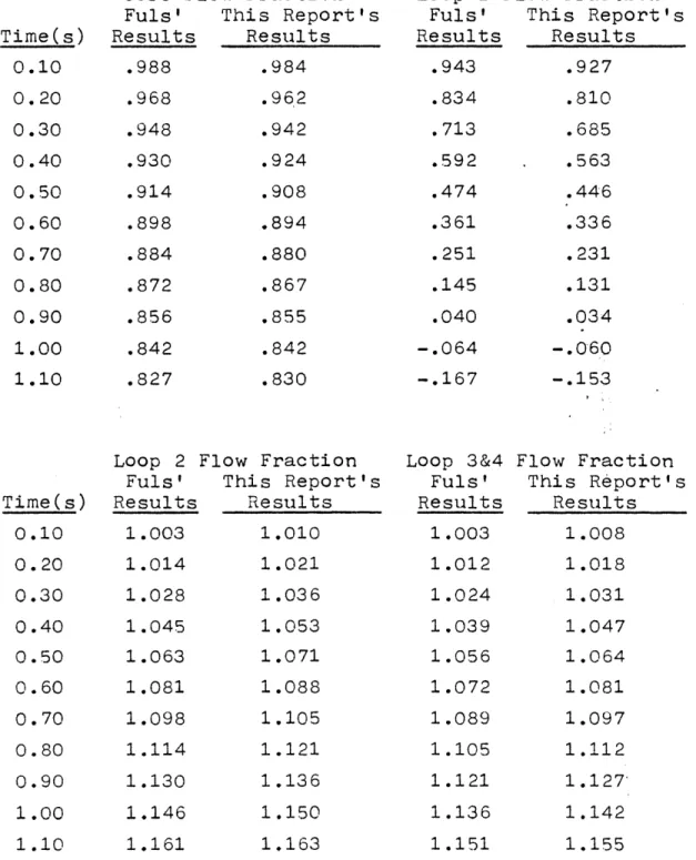
The results given in table 6.1.1 for core flow differ no more than 0.6% from those of Fuls. This seems adequately close to give one verification point for the computer program.

The derivation demonstrates an alternate way of specifying the BHP curve (by supplying the hydraulic power and impeller losses).

42

Table 6.1.1.Results for the Example from Fuls' Report

Initial Flow Values

Loops 1&2 initial flow = 793 kg/s

Loops 3&4 initial flow = 810 kg/s Core initial flow = 3206 kg/s

Time(s) 0.10 0.20 0.30 0.40 0.50 0.60 0.70 0.80 0.90 1.00 1.10 Time(s) 0.10 0.20 0.30 0.40 0.50 0.60 0.70 0.80 0.90 1.00 1.10

Core Flow Fraction

Fuls' This Report's Results Results .988 .984 .968 .962 .948 .942 .930 .924 .914 .908 .898 .894 .884 .880 .872 .867 .856 .855 .842 .842 .827 .830

Loop 2 Flow Fraction Fuls' This Report's

Results Results 1.003 1.010 1.014 1.021 1.028 1.036 1.045 1.053 1.063 1.071 1.081 1.088 1.098 1.105 1.114 1.121 1.130 1.136 1.146 1.150 1.161 1.163

Loop 1 Flow Fraction

Fuls' This Report's Results Results .943 .927 .834 .810 .713 .685 .592 .563 .474 .446 .361 .336 .251 .231 .145 .131 .040 .034 -. 064 -. 060 -. 167 -. 153

Loop 3&4 Flow Fraction Fuls' This Report's Results Results 1.003 1.008 1.012 1.018 1.024 1.031 1.039 1.047 1.056 1.064 1.072 1.081 1.089 1.097 1.105 1.112 1.121 1.127 1.136 1.142 1.151 1.155

43

6.2.Maine Yankee Reactor

The pump model and computational model has been applied to the analysis of the Maine Yankee reactor. In this example, there are two situations; one is that only one pump fails; and the second is that all the pumps fail. Information on the reactor was found in the Maine Yankee Reactor FSAR(t0) and also from information provided by the Yankee Atomic Electric Company(t).

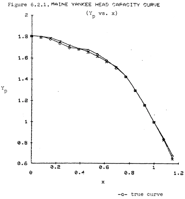
6.2.1.Maine Yankee Head-Capacity Curve

The Maine Yankee head-capacity is given in figure 6.2.1 and in table 6.2.1 .

The functional relationship between Y and x is chosen

p

to be quadratic:

2

We solve for C1 and C 2 by choosing two points on the

given Yp , x curve.

Therefore the values for C 1 and C 2are:

C Pi ,p2 1 2 and C p2x _{p 2} - Yplx₂ 1- ₂

To improve the accuracy of the head-capacity curve we divided the curve into three regions.

C1 = -1.06

C2 2.06. (x0O. 7397)

For x between 0.308 and 0.7397

For x between 0.000 C = -. 53 C = 1.77. 2 an 0.308 C = -. 53 C 2 = 1.77 (0.3085x<0.7397) ( 0. OOx<0. 308 )

but for this range we add a correction term to the Y equation. This term is:

Yp

=

6Y

(1

-

Table 6.2.1.Maine Yankee Head-Capacity Curve Rated Values

WR = rated loop flow = 6061 kg/s

ApR = rated pump pressure rise = 510 kPa

R = normal operation fluid density = 739 kg/m3

wR = rated pump speed = 125.7 rad/s (60 Hz) (Table given at y= 739 kg/m3 and w = 125.7 rad/s)

True Values Yp 1.81 1.80 1.78 1.74 1.70 1.69 1.68 1.64 1.58 1.51 1.43 1.30 1.16 1.00 0.84 0.68 Computed Values YP 1.81 1.80 1.79 1.76 1.72 1.69 1.66 1.62 1.57 1.52 1.43 1.30 1.16 1.00 0.83 0.65

(True values taken from curve provided in Maine Yankee(7))

x 0.000 0.077 0.154 0.231 0.308 0.385 0.462 0.539 0.615 0.692 0.769 0.846 0.923 1.000 1.080 1.150

46

Figure 6.2.1. MAINE YP'KEE HEAD CAPACITY CURUE

2- (Y vs. x) 1.8 1,4 1.4 I 0.8 0.8 1.2

-a- true curve -x- computed curve

47

6.2.2.Maine Yankee Brake Horsepower Curve

The Maine Yankee BHP curve is given in figure 6.2.2 and in table 6.2.2 .

Two straight lines fit between the following coordinate points (x,Y T) = (0.000,1.4), (0.367,1.0), and (1.000,1.0).

Therefore, the functional relationship between YT and x in this range is:

Y = x + C. T 3 4 For x equal to 0.00 to 0.367 C3 = -1.09 C. = 1.4 . (0 .000<xO.367)

For x between 0.367 and 1.00

C

=

0.00

C

c = 1.00

4

(0.367<x<l.000)

For x greater than 1.00, information was provided by Yankee Atomic Electric Co.(as prepared for a large break LOCA RELAP case). The functional relationship between Y Tand x for x greater than 1.00 is:

YT= C 5x + C6x2

For x greater than 1.00 but less than 2.00

C = 2.00

5

6= -1.00

48

For x greater than or equal to 2.00

C = 2.54

C = -1.40 (2.00ox)

From the information provided, there is a discontinuity occurring at x = 2.00. Work was not done on this discontinuity to determine its cause(s).

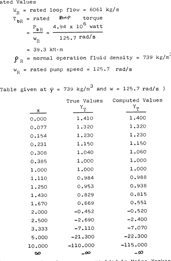
Table 6.2.2.fMaine Yankee BHP Curve Rated Values

WR = rated loop flow = 6061 kg/s T = rated 5HF torque

bR

P _DR 4.94 x 106 watt wR 125.7 rad/s

= 39.3 kN-m

PR = normal operation fluid density = 739 kg/m

3

wR = rated pump speed = 125.7 rad/s

(Table given at Y = 739 kg/m3 and w = 125.7 rad/s )

True Values Computed Values

x T T 0.000 1.410 1.400 0.077 1.320 1.320 0.154 1.230 1.230 0.231 1.150 1.150 0.308 1.040 1.060 0.385 1.000 1.000 1.000 1.000 1.000 1.110 0.984 0.988 1.250 0.953 0.938 1.430 0.829 0.815 1.670 0.669 0.551 2.000 -0.452 -0.520 2.500 -2.690 -2.400 3.333 -7.110 -7.070 5.000 -21.300 -22.300 10.000 -ii0.000 -115.000 Wo _oo -00

(True data taken from curve provided in Maine Yankee( 7) and from curve provided by Yankee Atomic Electric Co.'s

50

Figure 6.2.2.MAINE YANKEE BHP CURUE (YT vs. x)

0.8 1.2 1.6

-o- true curve

-x- computed curve 1.6 1.2 I e.6 0.4 yT -0.6

6.2.3.Maine Yankee Net Positive Suction Head Curve

The Maine Yankee NPSH curve is given in figure 6.2.3 and table 6.2.3.

The functional relationship between Y and x is chosen to be quadratic:

Yp = C₇ x2 ₊ C8 .

Solving for C7 and C8 from the graph(figure 6.2.3) the

values of the constants are:

C = 1.15

52

Table 6.2.3.14aine Yankee NPSH Curve Rated Values

WR = rated loop flow = 6061 kg/s

PR = normal operation fluid density = 739 kg/m3 wR = rated pump speed = 125.7 rad/s

p'R = rated NPSH = 438 kPa

(Table given at P = 739 kg/m3 and w = 125.7 rad/s )

True Values Computed Values

x Yp' YP'

1.040 1.09 1.09

1.140 1.33 1.33

1.25 1.64 1.64

53

Figure 6.2.3.MAINE YANKEE NPSH CURUE

(Y p'I vs. x) 1.05 1.15 1.1 1.2 1.25 1.3 -0- true curve -x- computed curve 1.6 1.5 1.4 p' 1.3-1.1 1 --i .7 T

54

The general mass flow equation (equation(3.1e)) is:

(LRV) dWRV (Li) dWL

(AR dt (A) dt _i

RVi iRV Ai ip

The pressure drop across each component in the loop can be due to friction and to shock.

friction pressure loss

The general equation for friction pressure drop (equation(3.1b)) is:

L(flWIW)

The friction factor f is determined from a Moody plot from Rust(29),figure4.1. _{First, the value of -/D is} determined for the component considered. Then the values of the friction factor f is plotted versus the Reynolds number on log-log paper. From this graph, a formula for the friction factor can be determined as a function of mass flow.

shock pressure loss

The general formula for shock pressure drop

(equation(3.1c)) is:

(P)jh

2WjW

sh= 2A2_f

To determine K, the pressure drop formula is set equal to its normal operation value.

All K values are considered constant (i.e. they do not change when flow changes).

Table 6.2.4.Maine Yankee Reactor Pressure Losses (kPa)

Full Flow, Zero Power, Average Temp. = 288 C

(ref. - Maine Yankee (I0))

component friction shock total

two stop valves 20.6 20.6

piping 15.4 48.7 64.1

steam generator 255.1

tubes 210.5 15.3

plenums 29.3

reactor vessel 170.2

inlet & 90Gturn 39.3 thermal shield 5.0 3.2

lower plenum 40.7

core 31.8 2.6

core spacer 12.3

o.utlet & nozzles 35.3

262.7 247.3 510.0

56

each component in the loop. stop valves K=Wsh L ~

#

no. of stop valves/loop = 2

(CP)sh =

(5.63x10 -4) _{W L} W L

piping friction loss

L( flWLI L (Zp)fr A 2Dh

p=

I-0.

piping shock loss - this loss is due to the two 900 turns the coolant does in going from the steam generator to the pump.

KIp)WL _{I WL of 90 turns)}

f= 739 kg/m3

A = .569 m 2 K = .32

(P)sh= (1.326x10 -3 )WL W

steam generator tube friction loss

L(fIWLI

L

E:/D = smooth tubing

f = f 4 = (4.277x10-2 )WL I -0.1 5 7

(LP)fr = (.526)f 4 IWL IWL

steam generator tube shock loss - this shock loss is due to entering and exiting the tubes. To determine the K's (one for entering and one for exiting) Q-(ratio of tube area to area at tube entrance or exit) is determined first. Then the values of the K's are determined from Rust(1L),figure 4.5.

Sp(K _{+ K C )(IVWL} 2Ap

S=

K c= entrance loss constant = .275

(Zp)sh=(4

.165x10 -4 ) _{W L} IWL

steam generator inlet and outlet plenum shock loss - this loss is due to the flow going from the inlet pipe to the

inlet plenum and from the outlet plenum to the outlet pipe.

K

fJWL

( P)sh

_2A2

reactor vessel (RV) inlet nozzle and 90 turn shock loss K LfWL ( sh _{2A 2} 2A = 739 kg/m3 A = .569 m 2 K = .51 (z p)= (1.07x10-3 _{)1W IW} sh L L

RV thermal shield shock loss - this loss is due to the coolant entering and exiting the thermal shield area. A pressure drop calculation was done indicating how the flow divides between the outer passage (reactor vessel & thermal shield) and the inner passage (thermal shield core core support barrel). Seventy-eighty percent of the total reactor vessel flow goes through the outer- passage. Also in order to

59

determine the K's, c- was calculated and the K's were determined from Rust(12.),figure 4.5.

(Ke + KClfW TSI TS ( )sh ₂₂ 2A = 739 kg/m A = 1.73 m 2 c7 - .78 K = 05 K - Sum adjusted to 0.47 x 0.15 = .071 W .78W TS = R ( p)sh = _{(2.06x10 -5) IjWR lWR}

(The value of the thermal shield shock pressure loss using this formula was higher than the normal operation value. Therefore, we multiplied the shock loss equation by .47 to equal the normal operation value)

(Ap) = (9.767x1q - 6 W IW

sh RV RV

RV thermal shield friction loss

L(fIWTIWTs) 2A _Dh = 739 kg/m A = 1.73 m2 L = 4.68 m Dh = .26 m C/D = .00017 f = f = (1.204x10-2)I I-.069 W =- .78W RV

( p)f p

(2.476x1-3 )f

w RW R

RV lower plenum loss

PIWv PWv

(Ap) = Po

₂

Apo

L(lWf WRVWRV) fr _2A2_Dh)

9-

core shock loss

(Ke + K ) IWRvI RV 2A2 = 739 kg/m 3 A = 4.95 m2 -=- .63 K = .14 e K = .15 C

(Ap = (8l1x10 - WRV WRV

core spacer loss - there are pressure loss due to the spacers supporting the fuel rods in the core. This formula for spacer pressure drop loss is from Rust(33),eq. 4.2.57. The equation for Cv was determined in the same way as the friction factors were determined.

CP E21w RVIWRV

(p)sp _2A2

3 2

= 739 kg/m,A = 4.95 m

= ratio of projected grid cross section to undisturbed flow cross section

2 D2

P - t

P = pitch = .0148 m

t = thickness of spacer walls = .77 mm

D = .0112 m & = .184

C = modified drag coefficient

= 54.86 I-.0245

(Ap) s = _{(7.481x10 -6)cvIW)}

I WR

core outlet region and nozzle shock loss

KWL IL

(p)sh ₂

S=

A = .569 m

(CaP)sh= (9.61x0-4) IWL IW_L

pump - the pressure loss is equal to the pressure head delivered by the pump. This is equal to the head-capacity curve in section (6.2.1).

Inertance Values (Maine Yankee(lO)) stop values a)L = length = 0.0 m piping a)L= 13.38 m b)A = area = .569 m2 steam aenerator a)tube length = 15.91 m tube area = 1.104 m2

b)inlet and outlet plenum length = .83 m inlet and outlet plenum area = .72 m2 pump a)L = 0.0 m reactor vessel a)90 turn L = .74 m 90 turn A = 3.42 m2 b)thermal shield L = 4.68 m thermal shield A = 1.73 m c)lower plenum L = 3.38 m lower plenum A = 6.16 m2 d)core L = 3.47 m core A = 4.95 m2

63

e)core outlet L = 1.99 m core outlet A = 4.95 m 2

6.2.5.Pump Speed Euation

The pump speed equation (equation (2.4h)) is: dw

I -= T -T - T

Pdt e b w

dt

where

I = moment of inertia of rotating parts of pump

= 4214 kg.m2

windage and bearing torques (T ,)

Equation (2.4g) is used for these torques. They are:

T = TR (w/w )2 w>.19wR

w wR

= .035TwR _O<w<.19wR

= .1TwR w = 0

T and w are the normal operation values of the

wR R

windage and bearing torques and pump speed. They are (information not available, therefore arbitrarily set to 2%):

TwR = .02 (Tb_R )

= .02(39.3 kN m)

= 787 N m

wR = 125.7 rad/s

BHP torque (Tb )

64

electric torque (TeR)

The electric torque equation (equation(2.4f)) is:

Te = TeR (e-t/ ) (w/wR )

where

T = normal operation value of electric eR

torque

= TbR + TwR

= 40.1 kN.m

tau = time decay of electric torque = it is an input into the program

-7

=

10

6.2.6.0ne Pump Failure Transient

In this situation, one pump fails. The object of the problem is to determine how the reactor vessel flow changes with time and to compare these results with results obtained

from the Maine Yankee FSAR(10).

The inputs to the program for this case is:

tau = electric torque time decay constant -10

= 10 -7 s

dt = time increment

= .1 s (see section (4.1)) limit = no. of time increments

= 80

n = total no. of pumps

np = total no. of failed pumps = 1

d = pump resistance constant

-5

The results from this report and the true values are shown in table 6.2.5 and figure 6.2.4. There is a kink occurring at a core flow fraction of 0.915. The cause of this kink could be due to the dividing of the head-capacity curve into three regions. Work was not done to determine if this was the cause of the kink.

Table 6.2.5.Results for Maine Yankee One Pump Failure Transient Time(s) 0.5 1.0 1.5 2.0 2.5 3.0 3.5 4.0 4.5 5.0 5.5 6.0 6.5 7.0 7.5 8.0

MIaine Yankee FSAR( \O) Core Flow Fraction

0.990 0.985 0.980 0.975 0.963 0.950 0. 943 0.935 0.933 0.920 0.915 0.910 0.903 0.895 0.880 0.875 Computed Values Core Flow Fraction

0.990 0.979 0.968 0.957 0.948 0.939 0.930 0.922 0.918 0.917 0.915 0.910 0.903 0.897 0.891 0.885

67

Figure 6.2.4llINE YANKEE ONE PUMP FAILURE

0.99 0.97 e 0.96s f a 0.92 c3 ₂ ± 0.91 0.88 I 1 ( 1 I i ' t 1 3 5 7 0 2 4 6 8

-o- true curve -x- computed curve

6.2.7.Complete Loss-of-Flow Accident

In this situation, all the pumps have failed. The object of the problem is to determine the reactor vessel flow versus time and to compare these results with those obtained from the Maine Yankee Start-Up report(11).

The inputs to the program are the same as in section 6.2.6 except that np equals 3.

The results from this report and the true values are shown in table 6.2.6 and figure 6.2.5. There is a kink occurring at a core flow fraction of 0.74. The cause of the kink could be due to the dividing of the head-capacity curve into three regions. Work was not done to determine if this was the cause of the kink.

69

Table 6.2.6.Results for Maine Yankee Complete Loss-of-Flow Accident Time(s) 0.0 1.0 2.0 3.0 4.0 5.0 6.0 7.0 8.0 9.0 10.0 12.0 13.0 14.0 15.0 20.0 25.0 30.0 40.0 50.0

Maine Yankee Start-Up( I ) Core Flow Fraction

1.00 0.94 0.89 0.83 0.78 0.74 0.70 0.66 0.62 0.60 0.57 0.53 0.51 0.49 0.47 0.39 0.34 0.30 0.29 0.28 Computed Values Core Flow Fraction

1.00 0.94 0.88 0.82 0.77 0.74 0.73 0.70 0.67 0.64 0.61 0.56 0.54 0.52 0.50 0.42 0.37 0.32 0.26 0.22

70

Figure 6.2.5.MAINE YANKEE COMPLETE LOSS-OF-FLOW ACCIDENT

0.9 0.8 0.7 0.6 0.5 0.4 0.3 10 15 30 35 40 45 SO time(s) -x- true curve -0- computed curve

6.2.8.Conclusions

For the one pump failure case the results in table 6.2.5 differ from the true values by no more than 2%. This seems adequately close for the pump model to be useful to model the Maine Yankee Reactor during this kind of transient.

For the complete loss-of-flow accident - the results from 0 seconds to 35 seconds are also very close (within 8%) to the true values. After 35 seconds the calculated values begin to fall under the true curve. There is no apparent explanation for this discrepancy. Natural convective processes are probably unimportant in this flow range. It does seem that the experimental curve changes slope in a manner not incorporated in the modeling.

7.CONCLUSIONS AND RECOMMENDATIONS

The performance of a reactor coolant pump has been adequately represented. By using dimensionless quantities,

equations have been developed to represent each

characteristic curve. The inertances and the pressure losses of the reactor loops have also been modeled. Using this loop model and the pump model, flow values have been predicted during plant transients.

Further work must be done on the pump model to handle cases of flow reversal in the loop. The pump resistance constant was arbitrarily set equal to-5 in all the examples in Chapter 6 and must be determined more precisely. The electric torque is generally assumed to go instantaneously to zero during pump failure. This assumption was made in all the examples but more information must be obtained to test the validity of this assumption. Thermal bouyancy features should be incorporated in the models. This will permit the calculation of portions of transients in which natural circulation becomes important. A final recommendation is to extend this single phase model to possible two phase situations. The work of Wilson(13) should be incorporated in

73

APPENDIX A COMPUTER PROGRAM USED FOR EXAMPLE FROM FULS' REPORT

A.1.Nomenclature

c

c al mass flow through each loop-initial value c a2 (L/A) values for each loop

c a3 coefficient used in change of mass flow equation

c

c d pump resistance constant - used when flow c reverses in pump

c delm change in mass flow at time tl

c dmI mass flow through the loop at time tl c dwl change in pump speed at time tl

c dt time increment

c

c flowl subroutine that determines the change in loop mass flow c and the change in pump speed in the failed pump

c flowill subroutine that determines the change in mass flow c in the loop that contains the nonfailed pump

c

c hc pressure rise delivered by pump

c

c limit number of time increments

c

c n total number of pumps

c np total number of failed pumps

c

c t absolute time after the first pump fails c tau time decay constant of electric torque

c tl absolute time after the first pump fails c twb windage and bearing torques

c

c wl pump speed at time tl c wr rated pump speed

c w4 mass flow through the reactor vessel

74

A.2.Program Listing

dimension tl (4),wl (4),dmi (4),dwl (4),delm(4) rewind 10

rewind 11 rewind 12 rewind 13 write(6,10)

10 format(lx,"enter tau,dt,limit,no. of pumps, no. of pump &failures, and pump resistance constant")

read(5,11)tau,dt ,1imit,n,np,d 11 format(v)

c initialize all the pumps-mass flow in kg/s,pump speed in s-1 do 40 l=1,n tl(l)=0.0 wI(1)=188.5 if(l.le.2)go to 20 a1=813.7187 go to 30 20 al=797.5061 go to 16 30 continue dml (1)=al dwl (1)=0.0 delm(1) =0.0 40 continue

c write headings of all the failed pumps k=1 if(np.It.l)go to 50 write(10,12) k,tl (k) ,wl (k) ,dml (k) if(np.1t.2) go to 60 write(11,12) (k+l) ,tl (k+l) ,wI (k+l) ,dml (k+l) if (np.lt.3) go to 70 write(12,12) (k+2),tl (k+2),wl (k+2),dml (k+2) if(np. lt.4) go to 80 write(13,12) (k+3),tl (k+3),wl (k+3),dml (k+3) 22 format(///,30x,"pump number",2x,12,///,20x,"failure

& at time",lx,flO.4,1Ox,"s",//,10x,"Initial pump speed",lx

,flO.4,lx,"s-1",//,lOx,"Initial mass flow",lx,flO.4, &lx,"kg/s",///, 18x,"Time", 1x," (s)",27x,"Pump Speed" &,1x,"(s-1)",22x,"Mass Flow", lx," (kg/s)")

go to 90

c write headings of all nonfailed pumps 50 write(10,14)k,wl (k),dml (k)

60 write(11,14) (k+l),wl (k+1),dml (k+l) 70 write(12, 14) (k+2) ,wl (k+2) ,dml (k+2) 80 write(13, 14) (k+3) ,wl (k+3) ,dml (k+3)

& pump speed",lx,fl0.4,lx,"s-1",//,10x,"Initial mass flow", &lx,f 10.4, lx,"kg/s",///, 18x,"Time", Ix," (s)",27x,

&"Pump Speed",lx,"(s-1)",22x,"Mass Flow",lx,"(kg/s)") continue

t=0.0

do 190 j=1,limit t=t+dt

if(np.eq.0.O)go to 110

flowl determines mass flow through and pump speed of the failed pump

do 100 k=1,np

call flowl(tau,dt,tl,wl,dml,dwl,delm,k,n,np,t,d) continue

if(n.eq.np)go to 130

flowil determines mass flow through the nonfailed pump do 120 k=l,n-np call flowll(dt,tl,wl,dmi continue ,dwl,delm,k,n,np,t,d) do 170 k=1,n do 160 l=1,n if(k.le.2)go to 140 a2=480.32 go to 150 a2=429.64 go to 150 continue if(k.ne.l)delm(k)=delm(k)-(18.86/a2)*delm(l) continue continue

update the mass flow through the do 180 k=l,n

dm I (k) =dm I (k)+de lm(k)

if (wl (k). le.O.O)wl (k)=O.O continue

failed and nonfailed pumps

write the time, pump speed, and mass flow of all the pumps write(10,13) t,wl (1),dml (1) write(11,13) t,wl (2) ,dml (2) write(12,13) t,wl (3),dml (3) write(13,13) t,wl (4),dml (4) format(15x,2(flO.4,30x) _,flO.4) wr i te (15, 15)dwl (1) format (v) continue stop end 100 110 120 130 140 150 160 170 180

c flowl determines mass flow through and pump speed c of failed pump

subroutine flowl(tau,dt,ti,wl,dml,dwl,delm,k,n,np,t,d) dimension tl (4),wl (4),dml (4),dwl (4),delm(4)

wr=188.5

c determine pressure head delivered by pump

hc=31.94*wI (k)**2-4.916E-01*dml (k)**2

if (dml (k) .le.O.O)hc=-(d*(5.45E-02)*dml (k)*abs (dml (k))) c determine windage and bearing torques

if (wi(k).ge.35.27) go to 20 if(wl (k).lIt.0.0) wl (k)=0.0 if(wl(k).eq.0.0) go to 30 twb=23.21 go to 40 20 twb=1.866E-02*wl (k)**2 go to 40 30 twb=66.315 40 continue

c determine change in pump speed

dwl (k)=(dt/16.94)*(-1.318E-03*dml (k)*hc*wl (k)/wI (k)**2

6-1.24*((.19)*wl (k)-(1.198E-02)*dml (k))**2-twb) c determine mass flow through the reactor vessel

50 w4=0.0 do 60 l=1,n w4=w4+dml (1) 60 continue

c update pump speed

c update pressure head delivered by pump w (k)=w I (k)+dwl (k)

hc=31.94*wI (k)**2-4.916E-01*dml (k)**2 c determine change in mass flow

if(k.le.2)go to 70 a 1=480.32 a2=2.51E-01 go to 80 70 al=429.64 a2=2.815E-01 go to 80 80 continue

de m (k) = (dt/al)* ( (-6.194E-02) *w4*abs (w4)

77

1 return end

c flowll determines mass flow through nonfailed pump subroutine flowll(dt,ti,wl,dml,dwl,delm,k,n,np,t,d) dimension tl (4),wl (4),dml (4),dwl (4),delm(4)

m=np+k

c determine mass flow through the reactor vessel w4=0.0

do 60 l=1,n

w4=w4+dmI (1) 60 continue

c determine pressure head delivered by pump hc=31.94wI (m)**2-4.916E-01*dml(m)**2

if (dml (m) . le.O.O)hc=-(d*(5.45E-02)*dml(m)*abs (dmi(m)))

c determine change in mass flow if(m.le.2)go to 70 a1=480.32 a2=2.51E-01 go to 80 70 al=429.64 a2=2.815E-01 go to 80 80 continue

delm (m) = (dt/al) * ((-6.194E-02) *w4*abs (w4)

&-(a2)*dml (m) *abs (dml (m))+hc)

1 return end