Design and thermal modeling of a residential building

Design and Thermal Modeling of a Residential Building

Alice Su-Chin Yeh

Submitted to the Department of Mechanical Engineering in partial fulfillment of the requirements for the degree of

Bachelor of Science in Mechanical Engineering at the

MASSACHUSETTS INSTITUTE OF TECHNOLOGY June 2009

MASSACHUSETTS INSTRUiTE OF TECHNOLOGY

SEP 16 2009

LIBRARIES

) 2009 Alice Su-Chin Yeh. All rights reserved.

The author hereby grants to MIT permission to reproduce and to distribute publicly paper and electronic copies of this thesis document in whole or in part in any medium

now known or hereafter created.

Author... ... ...

Department of

Certified by ...

Esther and Harold E. Edgerton Assistant Professor of

Mechanical Engineering May 8, 2009 Evelyn N. ang Mechanical Engineering Thesis Supervisor A ccepted by ... .. . ... i. . . . . John H. Lienhard V Collins Professor of Mechanical Engineering Chairman, Undergraduate Thesis Committee

ARCHIVES

Design and Thermal Modeling of a Residential Building

by

Alice Su-Chin Yeh

Submitted to the Department of Mechanical Engineering on May 8, 2009, in partial fulfillment of the

requirements for the degree of

Bachelor of Science in Mechanical Engineering

Abstract

Recent trends of green energy upgrade in commercial buildings show promise for ap-plication to residential houses as well, where there are potential energy-saving benefits of retrofitting the residential heating system from single-zone to multi-zone tempera-ture control. The objective of this thesis is to design a physical model to simulate the thermal profile of a residential building with a conventional single-zone central heating system. A scale model of a 2-story house was designed and constructed at 1/20 of the length scale of an average lifesize house, with an external heater and five temper-ature sensors connected to Vernier LabPro for data acquisition. Comparison between scale model prediction and experimental result shows similarity in steady state values for temperature and characteristic heating/cooling time constants. This thesis is an important first step toward designing a model house for multi-zone heating studies.

Thesis Supervisor: Evelyn N. Wang

Acknowledgments

First, sincere thanks go to the author's Orange Team members, specifically Shreya Dave, Peter Wellings, Tiffany Tseng, Rebecca Smith, Rahel Eisenberg, and Aiko Nakano, for all the highs and lows of 2.009 and for providing inspiration for this the-sis. Gratitude also goes to Jane Kokernak for teaching the author that engineering is ultimately about building relationships with other human beings.

M. Alejandra Menchaca (Ale) and Tea Zakula from the Building Technology Lab helped formulate the design process early on. Their advice was critical throughout this project. Professor Maria Yang and Justin Lai kindly agreed to provide lab space necessary for storing the equipment and running the experiment. They have saved the author an enormous amount of time.

Dr. Barbara Hughey was always so quick with dispensing tempor sensors and helping with relays. Thea Szatkowski and Michelle Lustrino provided the moral support during the intense thesis-writing time. Judy Yeh, the best sibling anyone could ask for in the world, provided wisdom and strength throughout the whole process. Thank you all for everything.

The author would not have gotten to this point without her academic advisor, Professor Dan Frey, for being a guiding light for her four years at MIT, and the academic support staff, espeically Dean James Collins.

Lastly, the author would like to thank Professor Evelyn Wang for teaching her 2.005 and 2.006, for being such a great role model, and for all the conversations in her office, whether related to academics or not. Thank you for being such an awesome thesis

Contents

2.2.1 Matching Non-Dimensional Numbers ...

2.2.2 Material and Corresponding Thickness . ...

2.2.3 Total Heat Transfer Loss & Volumetric Flow . 2.3 Assumptions Made in Design . ...

2.3.1 Radiation Effect ... ... 2.3.2

2.3.3

Natural Convection Effect Assumed to be Negligibl Well-Mixed Air . . . ... 11 ... . . 11 .. . . . 12 .. . . . 13 .. . . . 15 .. . . . 17 .. . . . 18 .. . . . 19 . . . . . 21 .. . . . 22 .. . . . 22 le . .. . . . . 22 .. . . . 22 3 Data Collection 3.1 Overview ...

7

3.2 Equipment and Software ... ... 23

3.3 Experimental Set-Up ... ... . 24

3.3.1 Transient Responses ... .. . . 25

3.3.2 Temperature Profiles Given Switching Control . ... 28

4 Analysis & Discussion 31 4.1 Overview. ... ... .. 31

4.2 Qualitative Observations ... ... 31

4.3 Steady State Temperature Comparisons. . ... 32

4.4 Time Constant Comparison ... ... 33

4.5 Discussion ... ... .. 35

4.6 Future Work ... ... ... 36

8

Chapter 1

Introduction

While more advanced commercial buildings currently have digital control of each room, residential houses have largely been ignored in terms of green energy upgrade. Most residential houses have traditional forced air heating system, with leaky rooms and inappropriately placed thermostats, and where most frequently occupied spaces rarely achieve their desired temperatures. As a result, the electricity cost and energy con-sumption are higher than necessary while human comfort is also compromised.

The inspiration for this thesis project came as a follow-up to the 2.009 (Product En-gineering Processes) course taken in Fall 2008. The Orange Team's product, Ther-moSmart, is a retro-fit smart grate system that effectively turns a single heating zone residential house into a multi heating zone home. Studies of heating systems are par-ticularly interesting because of their practical connections to thermodynamics, heat transfer, and fluids engineering. Originally conceived as a project dedicated to experi-mentally validating the hypothesis that the homeowner saves -10% in energy bill after transforming the house from single-zone to multi-zone, the project has been scaled back.

The objective of this thesis is to design and construct a scaled, physical model of a residential house as a first step toward studying multi-zone heating control.

According to Etheridege et. al. [6], there is a trend in building technology research toward using computer simulation models instead of physical models. The main ad-vantages for computer simulation include money and time, easier-to-control conditions,

and knowledge of specific points of interest. Computation fluid dynamics (CFD), one of the methods of computer modeling, replicates the system behavior with little or no equipment. Furthermore, it is not constrained by the viability of thermocouples or any sensors, and in principle, provides precise information (e.g., temperature, velocity, pressure) at every point spatially and temporarlly.

However, physical models offer advantages because computer simulations are prone to "noise," or any perturbations in initial set-up. If any given parameter is not specific precisely, the result can come out wrong and the simplest condition cannot be repli-cated. While the design of a physical model tend to be more general and the data less precise, physical data cannot be argued. Physical data directly measures the state of the system regardless of whatever models or values used. Last but not least, the in-trinsic satisfaction derived from building something by hand cannot easily be replaced by virtual models.

With the above discussion in mind, this thesis project focuses on the design and thermal modeling of a residential building and with experimental data collection.

Chapter

Design

2.1

Framework

The objective of this project is to design and construct a physical model to simulate the thermal profile of a residential building. To accurately model the thermal behavior of a building, it is important to understand what parameters are important. The following

are steps used in the design process specifically for this project.

1. Declare parameter of interest. 2. Model physical situation.

3. Extract all important parameters. 4. Find non-dimensional numbers.

5. Determine critical non-dimensional numbers. 6. Scale from life-size building to model.

The most important parameter of interest is temperature (human comfort most directly effected by temperature of the room)1.

1

According to [10], there are four environmental factors to comfort: temperature, humidity, air motion, and radiation. The focus here is on temperature.

2.1.1

Modeling

A simplified model of a house for this project is shown in Figure 2-1,

b Pair Pfair Tkb kair cp Troom Vair, in Vair, house Dh AP Lhouse T in _ir, __ Lduct

Figure 2-1: Simple Physics Modeling

where the parameters are as follows:

Tamb _{: Temperature of the ambient environment [oC]}

Troom : Temperature of the room (assumed uniform (see section 2.3)) [oC]

Tair,in _{: Temperature of the air when it enters the room [oC]}

Pair : Density of air [ k]

kair : Thermal conductivity of air [Watt] cp : Specific heat capacity of air [Watt]

Pair : Viscosity of air [Pa - s]

vair,in : Velocity of the air coming out of the grate/duct/pipe ["]

-Vair,house : Velocity of air along the wall/ceiling, here assumed to be M Vair,in

Dh : Hydraulic diameter of the tube that supplies the air to the room [m]

Lduct : Length of the duct from furnace (heater) source to room [m]

Lhouse : Characteristic length of the house [m]

AP : Pressure loss in the duct from furnace (heater) source to room [Pa]2 Note the relevant temperatures, Tamb, Tair,in, Troom.

2.1.2

Non-Dimensional Numbers

Non-dimensional numbers are inherently a comparison of the different forces at work and remain invariant regardless of the scale of the situation; therefore, non-dimensional numbers are used for scaling purposes. As will be discussed in detail later in section 2.2, it is important to design a life size house with specific dimensions and scale down to a physically manageable model. For a first order approximation, typical numbers are used to get a sense of what behavior is expected.

Given the model and associated parameters in section 2.1.1, three Pi groups3 can be extracted. The Pi groups are important because they are by design non-dimensional. The Non-Dimensional Numbers are the following:

Repipe : Reynolds Number of the pipe flow Repate : Reynolds Number of the flate plate. Pr: Prandtl Number

Tair,in-Troom _{The temperature comparison of the two gradients.}

Troom-Tamb

2

The pressure loss is the most significant loss and is a function of the major and minor losses through a pipe.

3

For a more in-depth discussion of Pi groups and the Buckingham Pi theorem please refer to [8] and [5]

The Reynolds number (Equation 2.1), by definition, compares the inertial and viscous forces in a pipe flow. Repipe a 2300 is the transitional regime where a value significantly above is considered turbulent and a value siginificantly below is considered laminar.

Replate is similar except that the geometry of the flow here is over a flat plate rather

than through a pipe. The transition number for Replate is w 6 x 104 [9]. Turbulent and laminar flows exhibit different flow patterns and have different heat transfer coefficients. Thus it is important to match this number.

vDh

Re = (2.1)

For the scaled down, physical model to exhibit approximately the same thermal be-havior, Reynolds numbers and temperature ratio need to be the same. For Reynolds numbers, it is important to have values on the same order of magnitude but the exact match is not essential4. Table 2.1 summarizes the parameters used in calculating the Reynolds numbers.

The Prandtl number, as defined in Equation 2.2, is a comparion of momentum diffu-sivity (kinematic viscosity) and thermal diffudiffu-sivity. It depends solely on the properties of the fluid. Therefore, since air is used in both life-size model and scale model, by design this dimensionless number is already matched.

Pr =1 (2.2)

a k

a is the thermal diffusivity of the air. Note that v is the kinematic viscosity of the liquid and equivalent to *

p

When Figure 2-1 is examined in more detail, it is reasonable to assume that Repipe is not as important given that what happens in the duct leading to each room is secondary to what happens in the room, thermally-speaking. The main point gathered from this discussion is that the small model needs to be scaled such that its Replate is on the

order of - 10' and that the temperature ratio Tair,in-Troom needs to remain the same. Troom-Tamb

4

Exact matching is not essential and in fact, a reasonable approximation can be made to match

Replate to 104.

Table 2.1: Expected Reynolds Numbers

Parameter Value

Pair

[-]

Pair [Pa -s] 1.8 x 10 same vair [- 2] 1.3 x 10 -5 same Dh [m] 0.14 -Lhouse [m] - 10 Vair,in [7-] 0.5 Vair,hosue [] - 0.5 Repipe " 5 x 103 Replate - 4 x 10s

2.1.3

Heat Transfer Processes Modeling

As mentioned before, it is important to design for the same turbulent or laminar flows because the heat transfer coefficients are significantly different. The heat transfer coefficient in laminar flows is rather low compared to that of the turbulent flows because turbulent flows have a thinner boundary layer on the heat transfer surface.

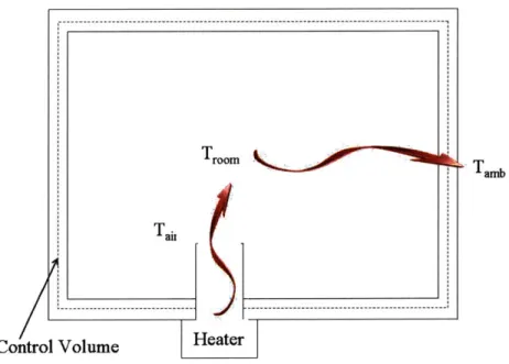
To design a simplified life size house, we start with the simplest case available, as shown in Figure 2-2: a room at a certain temperature Troom with warm air flowing in at a temperature Tair,in. By defining the control volume to be the boundary of the room, the energy equations can be applied to the system. The outside temperature is given by Tamb. The room loses

Q

out = UA(Troom - Tamb) (2.3)

where UA is the effective heat transfer coefficient (scaled by the flux area) in [Wt] and the temperature difference is Troom - Tamb. The effective heat transfer coefficient

U is the inverse of the effective resistance Ref [MWa,

-1

U = (2.4)

Figure 2-2: Heat Transfer Modeling

where the higher the material conductivity or heat transfer capability, the lower the resistance value. (R values will be used throughout in the design calculations later.) Comparatively, the furnace (given by "Heater" Figure 2-2) supplies air at a heat trans-fer rate of

Q.

Qin = ricW(Tair,in - Troom),

(2.5)

where rh [ ] is the mass flow rate from the heater, c, [ c] the specific heat capacity of air, and Tair,in. The mass flow rate, ri, is also the density of air p [ ] multiplied by volumetric flow rate V [

],

(2.6)

rm

=

pV

Qin=

The substitution of 1V for rh is done because 1V is an easier parameter to measure and work with later on in the design calculations.

For the room to remain at a desired temperature, the amount of heat transfer into the room must be equal to the heat transfer out of the room. Assuming no energy storage, Equation 2.3 is equal to Equation 2.5, or

Qout

Qin.

UAATout = pVcpAT (2.8)

There are many insights that can be gained from studying this equation, which will be discussed later in the section.

2.2

Life Size House and Scale Model House

In order to examine comparable quantities, it is necessary to first design a life-size house and then scale down to a physical model. A typical US residential house is about -2300 sq. feet [1], which translates to - 200 m2_{. If a typical house is assumed}

to have two floors (with each floor having a standard height of 10 feet or -3 meters, then each floor would have - 100 m2 of space. This is convenient number suggests a

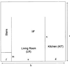
house with a 10 m x 10 m floorplan can be designed. Figure 2-3 shows the full house with all of the interior partitions. It is important to note that this diagram is not only the layout of the proposed life size house, but also is the layout of the scale model built for this project. Figure 2-4 and Figure 2-5 show the same information but with the function of each partition labeled5. All of the dimensional values and labeled with alphabetical letters and given in Table 2.2. Note that the scale factor used is 0.05. In other words, the scale model is 20 times smaller in length. Correspondingly, if the length is 20 times smaller, the area is 400 times smaller and the volume is 8000 times smaller.

5

The figures are not drawn to scale.

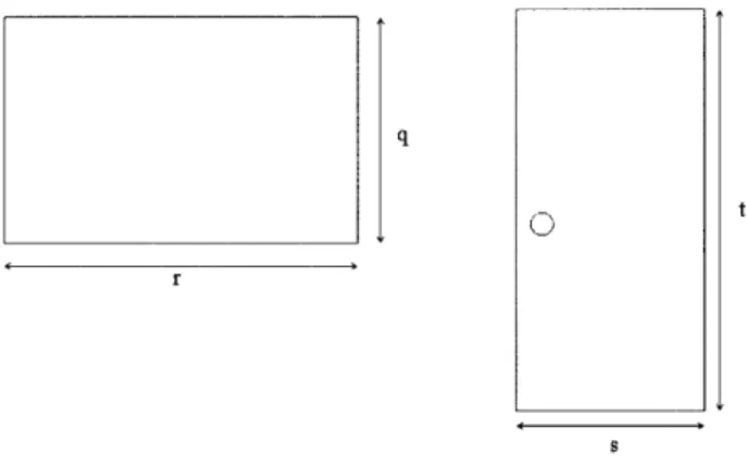
Although Figure 2-4 and Figure 2-5 do not show the windows and doors for the sake of clarity, there are a total of 10 windows, 1 main door, and 1 door for each bedroom and bathroom. The specific dimensions are labeled and also given in Table 2.2.

f

1F n a

f e

Front Door

Figure 2-3: House in 3D with Relevant Dimensions

2.2.1

Matching Non-Dimensional Numbers

As mentioned in section 2.1.2, the following non-dimensional numbers need to be matched in the design process: Tairn-Troom and Replate.

For a life size house, Tair,in - Troom is typically 10

"C

"C for a ratio of - 0.5. Therefore, this ratio will be the same for the model house. For a life size house, Repate 104, so for a model house with a characteristic length of 0.5 m, the velocity at which air enters the room should be 0.26m.

1F

cn

Living Room Kitchen (KIT) (LR) f e d b Figure 2-4: IF Floorplan g 2F

E Bedroom 1 Bed Room 2

(BR1) (BR2)

f h

b

Figure 2-5: 2F Floorplan

2.2.2

Material and Corresponding Thickness

To ensure the condition in Equation 2.8 is achieved, UA must be the same for both the life size and model size houses. In other words, the equivalent "resistance" (which combines all the conduction interfaces) through the wall, roof, and ceiling must be the

0

Figure 2-6: Window and Door Table 2.2: Dimensions

Label Life-Size House [m] Scale Model House [m] (scale factor 0.05x) a,b c,d e f,j ,m g,p h i k 1 n o q,s r t 10 3.0

5.5

1.5

8.5

4.5

7.0

Therefore, Tables 2.3 and 2.4 summarize the materials and thicknesses used with the approximate equivalent resistance for each section6

6

Values calculated and taken from [10].

Table 2.3: Req values of a Typical House Section Req [- -] Wall 2.0 Roof 0.7 Ground 3.3 Window 0.7

Table 2.4: Materials and Designed Thicknesses Used in Scale Model Material Thickness[m] Calculated Req

2.1 Wall Cardboard 0.003 Insulation 0.052 0.67 Cardboard 0.015 Insulation 0.015 Ground Cardboard 0.065 Insulation 0.065 0.68 Window Cardboard 0.017 Insulation 0.017

2.2.3

Total Heat Transfer Loss & Volumetric Flow

The total heat loss of the life size house is calculated to be 5000 kilowatts given the dimensions mentioned previously. Given this heat loss, the volumetric flow is then calculated to be about e 0.8 m . According to Bell [4], a typical house needs an additional 0.3 _ to account for leakages, bringing the total to 1.1 . The volumetric

ow for house, the model then, should be 400 times smaller, or

flow for the model house, then, should be 400 times smaller, or e 0.00275 M 3

2.3

Assumptions Made in Design

2.3.1

Radiation Effect

Radition losses can be safely assumed to be negligible because while its fourth power

temperature dependence is significant at high temperatures, for the temperature values

used here, radiation heat transfer is relatively small. In fact, according to [7], the heat

transfer coefficient is around 5

K for room temperature. The heat transfer coefficient

for forced convection (which is heavily prevalent in building heat transfer) is about 1-2

orders of magnitude larger.

2.3.2

Natural Convection Effect Assumed to be Negligible

Natural convection heat transfer coefficients are not easily predicted and involve

it-erations through correlations such as the Nussult number and Grashof number. In

addition, the effect of air flow entering the room is considered large enough that most

heat transfer will be through forced convection rather than natural convection.

2.3.3

Well-Mixed Air

Well-mixed air or uniform temperature within a room is assumed for the design of the

model. This is important, as having a temperature gradient in the room increases the

complexity of how a home thermal system can be modeled. This suggests that the

thermal boundary layer is considered small such that there is litte effect on the bulk

room temperature. Using the thermal boundary equation given by [5], the thermal

boundary thickness for the life-size house is approximately 90 cm and for the model

house, approximately 1 cm. Therefore, the boundary layer is thin and can be safely

assumed to be negligible.

Chapter 3

Data Collection

3.1

Overview

In the following chapter, a description of the experiment is given as well as a summary of the data collected.

3.2

Equipment and Software

The following equipment and software were used to carry out the experiments:

* Heater

Honeywell Air Heater (HZ-338) 120V A.C., 60Hz., 12.5A., 1500W

The heater supplies hot air to the model house. * Fan

Honeywell Three-Speed Fan (HTF-100 Series) 120V A.C., 60 Hz., 0.80A

The fan, placed in front of the heater, accelerates the hot air so that a higher air velocity can be supplied to the model house.

* Anemometer

Extech CFM Thermo Anemometer (Model 407114) Sampling rate: 1 reading per second approx.

Sensors: Air velocity/flow sensor: conventional angled vane arms with low-friction ball bearing

Range Specifications: in meters per second, range is 0.40-25.00 m/s with resolu-tion 0.01 m/s and accuracy ± 2% + 0.2 m/s)

* Temperature Sensor

Vernier Stainless Steel Temperature Probe (TMP-BTA) Temperature range: -40 to 135 'C

12-bit resolution(LabPro): 0.03 'C for 0 to 40 'C Temperature sensor: 20 kQ NTC Thermistor Accuracy: ± 0.2 'C at 0 °C Response time: 95% of full reading: 11 s 98% of full reading: 18 s 100% of full reading: 30 s * Data Acquistion

Vernier LabPro Hardware and LoggerPro 3.6.1 Software Logs data every 0.5 s

* Model

For more information on the design of the model, refer to the previous chapter.

3.3

Experimental Set-Up

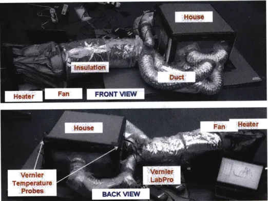
The experiment set-up is shown in Figure 3-1, with a Vernier temperature probe in each room(Bedroom 1, Bedroom 2, Kitchen, 2F Hallway, Living Room). The temperature probes were connected to the LabPro hardware, which interfaced a laptop to monitor

---the temperature continuously. The three settings on ---the fan allowed for three different

flow settings: minimum, medium, and maximum in flow intensity to examine the effect

on temperature.

Figure 3-1: Front and Back Images of Model Built

Two different sets of data were obtained: steady state temperature & time constant

of the building due to one heat load cylce and temperature profile of the house using

manual-based switching control.

3.3.1

Transient Responses

To find the transient response of the building, the heater is turned on until a steady

state temperature is reached. The heater is then turned off, allowing the temperature

of the house to fall until it reaches equilibrium, which is the ambient temperature. The

temperature changes as a function of time, each with a different flow setting, are shown

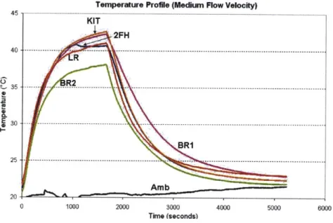
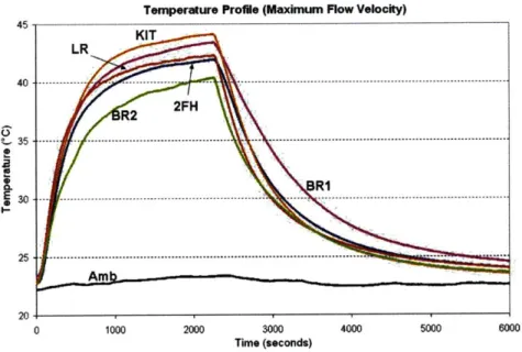
in Figures 3-2, 3-3, and 3-4.

Temperature Profile (Minimum Flow Velocity)

1000 2000 3000

Time (seconds)

4000 5000 6000

Figure 3-2: Temperature Profile (Minimum Flow Velocity)

Temperature Profile (Medium Flow Velocity)

0 1000 2000 3000

Time (seconds&

Figure 3-3: Temperature Profile (Medium Flow Velocity)

The air flow conditions were summarized in Table

3.11.

1

This airflow as it entered each room was not simply a linear airflow. It was more likely that some

45 40 30 25 20 45 40 1,35 -25 20 4000 5000 6000 ~

Temperature Proile (Maximum Flow Velocity) 45 KIT LR 40 ---R2 2FH 20 0 1000 2000 3000 4000 5000 6000 Time (seconds)

Figure 3-4: Temperature Profile (Maximum Flow Velocity)

Table 3.1: Measurement of Temp. and Room Velocity Entrance

Min. Flow Med. Flow Max. Flow

Location Tair,in(0C) vair,in Tairin(oC) Vair,inm Tair,inO Vair,in

Heater 58 1.46 53 2.49 55 2.67 BR1 44 1.46 44 0.68 44 0.87 BR2 48 1.46 45 0.55 47 0.78 LR 53 0.34 48 0.41 48 0.75 KIT 55 0.22 49 1 50 1 2FH 50 0.86 44 1.03 47 1.06

Referencing back to section 2.2.1, velocity needs to be at least vair,in " 0.24 in order for the Reynolds number to match. Table 3.1 shows that the velocities are in the range of and above that value. This suggests that the model has flow patterns also in the turbulent regime and therefore should have comparable heat transfer coefficients. The

temperature ratio, Tairn-Toomn is also comparable.

random flow motion, perhaps caused by the interior duct roughness, was present. This observation was from repeated attempts at getting an accurate reading on the anemometer. Many times, a reading can be obtained only by tilting the anemometer at various angles. Therefore, the velocity values given in Table 3.1 are only approximate values.

3.3.2

Temperature Profiles Given Switching Control

To observe how a scale model might behave with typical forced hot air heating system,

a room was chosen as the standard. Here, the 2F Hallway was chosen, analogous to

where the thermostat in a typical residential house would be placed.

When all rooms were at e 20 "C, the heater and fan were turned on. When 2F Hallway

reached 42 "C the heater and fan were turned off. When 2F Hallway reached 38 "C,

the heater and fan were turned on again. These steps were repeated for 4-5 cycles and

the rooms were allowed to come back to equilibrium.

In typical heating systems, switching control is used where a range is given. If the

system were to be controlled with only a set temperature, the furnace would be

con-stantly turning on and off, reducing its life expectancy. Instead,

and To", are

given as an offset from Tdesired so that the temperature will oscillate between the two

at a relatively low frequency.

For the experiment, Tdesired = 40 °C, Thigh was chosen to be 42 "C, and To,, was 38 "C.

The data collected are summarized in Figures 3-5, 3-6, and 3-7.

45 40 35 -. 25 20 15

Temperature Profile Based on 2F Hallway (Minimum Flow Velocky)

0 1000 2000 3000 4000

Time (seconds) 5000 8000 7000

Temperature Profile Based on 2F Hallway (Medium Flow Velocity) 45 2FH 40 BR1 BR2 LR KIT Amb 20 0 1000 2000 3000 4000 5000 6000 7000 Time (seconds)

Figure 3-6: Temperature Profile based on 2F Hallway (Medium Flow Velocity)

Temperature Profile Based on 2F Hallway (Maximum Flow Velocity)

0 1000 2000 3000 4000

Time (seconds)

5000 6000 7000

Figure 3-7: Temperature Profile based on 2F Hallway (Maximum Flow Velocity)

45 40 9- 35 0 I-25 20

~-II

-Chapter 4

Analysis & Discussion

4.1

Overview

A summary of the experimental set-up and data collected is given in Chapter 3(Fig-ures 3-2, 3-3, 3-4, and Table 3.1). The fig3(Fig-ures are the focus of analysis and discussion in this section.

4.2

Qualitative Observations

* Figures 3-2, 3-3, and 3-4 show exponential trends in temperature, where the time constants and steady state values1 can be analyzed. Time constants and steady state temperatures are the topic of further analysis in the next sections. * The different flow settings do not appear to make a difference in temperature

profile, rise time, or settling time.

* All monitored rooms exhibit same exponential trends with peak values of ± 5 'C difference. It is possible that the flow conditions are too close, and for significantly

different results, Tair,in, vair,in, and relative dimensions need to be at least one

order of magnitude different.

1_{the definition of time constant used here is the rise or settling time characterizing the response of}

a first-order linear time-invariant (LTI) system -i -;;- ;- ---- "

-* The control graphs (with the control of the furnace of one room only) show that the other rooms almost never reach the desired temperature ranges.

4.3

Steady State Temperature Comparisons

Predicted T,,

In finding the steady state temperature of the room, energy flow rates in and out of the system are connected (i.e., heat transfer into the house from the heater is equal to the heat transfer out of the house). In other words, in a steady state condition, the system is at equilibrium with the same amount of energy going in as energy going out. This is the model used in our design in Figure 2-1 and corresponding Equation 2.8. While the room temperature, Troom, is determined a priori in designing the scale model house,

Ts, is left as a value to be determined in this case.

Therefore, by using Equation 2.8 and rearranging it appropriately,

pVTair,in + UATamb

Troom,steadystate = (4.1)

pV + UA

If the whole house is considered as the system, the following values are substituted, as summarized in Table 4.1:

Table 4.1: Values for Ts8 Calculations Parameter Life Size House Model House

p [,]

1.15

1.15

30

45

For the life size house, T18 is calculated to be 26 "C. For the model house, T,, is calculated to be - 41 "C.

__-Experimentally measured Ts8

From Figures 3-2, 3-3, and 3-4, the steady state temperature (when average out all the temperatures looks to be 41 C, which is almost exactly the same as the expected value.

4.4

Time Constant Comparison

Predicted T

Applying conservation of energy to a control volume yields Equation 4.2 where Ein is the energy going into the system, E,,out is the energy going out of the system, and Ess is the steady state, internal energy. In the case of home heating system, the energy is in the form of heat transfer, which is shown in Equation 4.3. This is a lumped-parameter modeling, essentially looking at the heat transfer process as if it is a RC-circuit.

Ein - Eout - dE = ES, (4.2)

dt

dQs

din

- =out = QS (4.3)

When heat is applied, the system can be modeled as a thermal "circuit," shown in Equation 4.4, where T = Troom - Tamb is the equivalent resistance, and

Qst

equivalent "resistance" (to heat flow) through the walls. The mcp value is essentially the "capacitance" of the house, but quantifying mc (e.g. just that of the air mass or that of the air mass + walls) involves more complication.

dT

mcp- d + UAT = Q,, (4.4)

2

Like the circuit equation V = IR, here T = QR

i,

dT

7d + T = T (4.5)

dt

Equation 4.5 is an ordinary differential equation (ODE), and the solution is given in Equation 4.6

Troom - Tamb - Tss(1 - e- ) (4.6)

When supplied heat is stopped and system allowed to cool (analogous to turning off the heater), the system has the same modeling with a temperature decay instead of growth, but the same time constant.

Tabel 4.23 summarizes the time constant values calculated assuming different modeling conditions. Note that the first condition (Air Mass only) assumes house is a "lump" of air only with negligible wall + ceiling capacitance. All other conditions assume that insulation takes up significant value relative to house, so the volume of air is reduced to 50% of the volume of the house.

Table 4.2: Time Consant T Calculations with Different Modeling Assumptions Condition Description Model House T (s)

Air Mass Only 2770 140

Air+Wall - 40

Air+Wall+Insulation - 40

Air+Insulation - 40

Wall+Insulation - 500

Experimentally measured 7

From Figures 3-2, 3-3, and 3-4, the time constants differ significantly for the growth and decay portions. The growth time constant is . 370 seconds, and the decay time constant is - 740 seconds. Both values are on the same order of magnitude as the predicted time constant with the wall+insulation combination.

3

The wall+ceiling materials and thicknesses were chosen so that the model would have the equiv-alent "conductance" as that of the life size house. However, equivequiv-alent "conductance" does not mean equivalent specific heat capacitance, and so the values for life size house are not calculated.

-4.5

Discussion

As the objective of this thesis project is to design an experimental model as a first step

toward designing a model house to study multi-zone heating control, it is important

to see how close the scale model data compares to the predicted values. In comparing

the steady steady values, the scale model predicted temperature and experimentally

collected values are remarkably similar, with both saying that it would be about

41

C for the model house, which translates to about a 26 C for a life size house. This

is significant in that the scale model is accurate in showing how much heat should be

supplied to a house in order to maintain a steady state temperature. In comparing

the time constant, the experimentally collected values are in the range of the predicted

value if assuming that the capacitance of the wall + insulation is most significant

(rather than just the air mass). While this assumption is not true for a real house,

it is reasonable for the model house designed for this project. Given the scale and

the need to match equivalent conductance, the wall + insulation thicknesses are large

compared to the size of the size. As a result, the actual air mass is about 50% of

the volume of the house. Table 4.2 shows that when the air is taken into account,

the time constant is very small; in other words, that particular model predicts that

the house's characteristic heating/cooling time is less than 1 minute. However, if one

considers the capacitance of the wall+insulation combinations to be most significant,

then the time constant is somewhat reasonable, at around 8 minutes for the model

house. This prediction matches up reasonably well when compared to experimental

data. In addition, the model assumes that heating and cooling time constants would

be the same whereas experimental data shows that cooling time is significantly longer.

An explanation for this observation of the experiment is that in heating, the heater is

actively pouring hot air into the house whereas in cooling, the heat transfer relies on

dissipation only.

By comparing experimental and predicted values, the thesis achieves the stated goal

of taking a first step toward designing a model house suitable for multi-zone heating

studies.

4.6

Future Work

There are many possibilities for future work. First, for further comparison and match-ing, an experiment could be set up in which a complete heating cycle of a one-zone heating (comparable to a typical forced hot air heating system), is observed. Second, for ease of building and experimental set-up, instead of keeping the equivalent resis-tance value constant and varying the volumetric flow, it would be interesting to explore with scaling the equivalent resistance value as well. Third, to bring everything together and reconnect back to the original inspiration of this thesis project, a project dedicated to focusing on data analysis of a control algorithm developed for the multi-zone retrofit heating system for residential buildings would be interesting to do.

Bibliography

[1] Margot Adler. Behind the ever-expanding american dream house, July 2004. http://www.npr. org/templates/story/story .php?storyld=5525283.

[2] American Society of Heating, Regrigerating and Air-Conditioning Engineers, Inc., Atlanta, GA. ASHRAE Handbook, Fundamentals Volume, 2001.

[3] American Society of Heating, Regrigerating and Air-Conditioning Engineers, Inc., Atlanta, GA. ASHRAE Handbook, HVAC Applications Volume, 2003.

[4] Arthur A. Bell. HVAC: equations, data, and rules of thum. McGraw-Hill, 2000. [5] E Cravalho and John G. Brisson. 2.006 thermal-fluids engineering ii, 2008. Course

Reader for 2.006, Spring 2008.

[6] David Etheridge and Mats Sandberg. Building Ventilation: Theory and

Measure-ment. John Wiley & Sons, 'West Sussex, England, 1996.

[7] Leon R. Glicksman and John H. Lienhard V. Modelling and approximation in heat transfer. Course Reader for MIT Subject 2.52, September 2007, 2006. [8] Frank P. Incropera and David P. DeWitt. Fundamentals of Heat and Mass

Trans-fer. John Wiley & Sons, New Jersey, fifth edition, 2002.

[9] W.M. Kays and M.E. Crawford. Convective Heat and Mass Transfer. McGraw-Hill, 1980.

[10] Faye C. McQuiston, Jerald D. Parker, and Jeffrey D. Spitler. Heating, Ventilating,

and Air Condition Analysis and Design. John Wiley & Sons, New Jersey, sixth

edition, 2005.