Science Arts & Métiers (SAM)
is an open access repository that collects the work of Arts et Métiers Institute of
Technology researchers and makes it freely available over the web where possible.
This is an author-deposited version published in:
https://sam.ensam.eu
Handle ID: .
http://hdl.handle.net/10985/17990
To cite this version :
R PAIN, P-E WEISS, S DECK, Jean-Christophe ROBINET - Large scale dynamics of a high
Reynolds number axisymmetric separating/reattaching flow - Physics of Fluids - Vol. 31, p.125119
- 2019
Any correspondence concerning this service should be sent to the repository
Administrator :
archiveouverte@ensam.eu
Large scale dynamics of a high Reynolds number
axisymmetric separating/reattaching flow
R. Pain,1 P.-E. Weiss,1,a) S. Deck,1 and J.-C. Robinet2 AFFILIATIONS
1ONERA - The French Aerospace Lab, F-92190 Meudon, France 2DynFluid, Arts et Métiers, ParisTech, 75013 Paris, France
ABSTRACT
A numerical study is conducted to unveil the large scale dynamics of a high Reynolds number axisymmetric separating/reattaching flow at M∞= 0.7. The numerical simulation allows us to acquire a high rate sampled unsteady volumetric dataset. This huge amount of spatial and
temporal information is exploited in the Fourier space to visualize for the first time in physical space and at such a high Reynolds number (ReD= 1.2 × 10⁶) the statistical signature of the helical structure related to the antisymmetric mode (m = 1) at StD= 0.18. The main
hydrody-namic mechanisms are identified through the spatial distribution of the most energetic frequencies, i.e.,StD= 0.18 andStD≥3.0 corresponding to the vortex-shedding and Kelvin-Helmholtz instability phenomena, respectively. In particular, the dynamics related to the dimensionless shedding frequency is shown to become dominant for 0.35 ≤x/D ≤ 0.75 in the whole radial direction as it passes through the shear layer. The spatial distribution of the coherence function for the most significant modes as well as a three-dimensional Fourier decomposition suggests the global features of the flow mechanisms. More specifically, the novelty of this study lies in the evidence of the flow dynamics through the use of cross-correlation maps plotted with a frequency selection guided by the characteristic Strouhal number formerly identified in a local manner in the flow field or at the wall. Moreover and for the first time, the understanding of the scales at stake is supported both by a Fourier analysis and a dynamic mode decomposition in the complete three-dimensional space surrounding the afterbody zone.
I. INTRODUCTION
The study of axisymmetric afterbody flows is mainly motivated by aerospace problems.1–4Indeed, this geometry is a very simplified prototype of the main stage of a space launcher’s after-body. The understanding of the structure of turbulent shear flows with separa-tion and reattachment is of major importance for many engineering applications. In some configurations, the flow is the seat of pres-sure fluctuations resulting in large nonaxisymmetric aerodynamic forces on the structure. The aim of this work is to better understand the physical mechanisms responsible for these pressure fluctuations. Eventually, the knowledge of the spatial organization of the fluc-tuating flow field permits us to guide the design of flow control devices.
Separating/reattaching flows are characterized by the presence of a recirculation region, which is governed by a complex dynam-ics.5,6As it is often accompanied by a highly unsteady fluctuating pressure field, it is usually preferable to avoid such unsteadiness as
it may induce interfering vibrations on the geometry. Among the wide variety of separation/reattachment scenarios, flow separation induced by a leading edge has been well documented in the last decades. For instance, Armalyet al.7 carried out an experimental investigation of a 3D backward facing step flow and evidenced that the length of the recirculation bubble increases with the Reynolds number in the laminar regime, while it decays in the fully turbulent stage. Furthermore, the authors have put forward the limitations of 2D modeling of such flow atRe > 400 for the fact that the recir-culation region becomes three-dimensional. By extension to bluff body cases, axisymmetric backward facing step flows are of partic-ular interest since the fluctuations in the recirculation zone interact with the wall of the emerging cylinder and expose the geometry to unsteady loads. Deck and Thorigny8showed that there exist some
similarities between the subsonic two-dimensional backward facing step flow and its axisymmetric counterpart mainly in terms of the shear layer properties. They also performed a spectral analysis of the fluctuating pressure field for a few sensors located in the vicinity
of the recirculation zone. The authors derived some main frequen-cies whose energetic contribution evolves spatially. In particular, the pressure fluctuations at a normalized frequency based on the largest diameter of the geometryStD = 0.2 were shown to be associated
with the antisymmetric azimuthal modem = 1. Later, Weiss et al.9 extended the fluctuating pressure spectral analysis to the wall, which unveiled a highly energetic area forStD= 0.2 fluctuations related to
thevortex-shedding. Such an area was located approximately in the middle of the recirculation zone (0.35 <x/D < 0.75). A linear stability analysis conducted by the authors showed in addition the absolutely unstable nature of them = 1 azimuthal mode. This result corrobo-rates the investigations on a supersonic axisymmetric wake behind a bluff body by Sandberg and Fasel10who suggested the coexistence of both absolutely unstable global modes and convectively unstable shear-layer modes.
From the experimental point of view, Deprés, Reijasse, and Dussauge11 characterized the axisymmetric backward facing step flow at the transonic regime both in terms of statistics (mean and root mean square wall pressure coefficients) and of the spectral con-tent of the wall pressure signal. The flow conditions of this exper-iment are used in this paper. These authors revealed two main Strouhal numbers. The first one corresponds to the vortex shedding StD≃0.2, which they associated with an antisymmetric large scale formation by means of a two-point correlation. The second one is related to the convection of turbulent eddies in the shear layer at StD≃0.6. On top ofStD≃0.2, Deck and Thorigny8outlined the con-tribution of an extra low frequency phenomenon associated with the flapping motion of the mixing layer atStD≃0.07 observed by Driver, Seegmiller, and Marvin12 for a planar case. Although the overall unsteady flow phenomena have been addressed in the past, their spatial organization as well as their time evolution remains not fully understood. Indeed, the identification of characteristic mechanisms of highly turbulent flows is still a great challenge for experimentalists and numerists due to the wide variety of scales to deal with.
The wake developing downstream of a sphere, a disk, or more generally a bluff-body develops coherent energetic and compact hairpin type structures. This characteristic is particularly observed when the flow is incompressible or in a low subsonic regime. When the Reynolds number increases but remains at a moderate Mach number (subsonic), the wake initially dominated by hairpin struc-tures type (or double hairpin) disappears gradually giving way to structures such as vortex rings. In this regime, the large scales are rel-atively axisymmetric and intermediate scales developed from shear instabilities and nonlinearly in the form of vortex structures of the chevron or hairpin type (but much smaller than the previous ones). However, for higher Reynolds numbers ReD ≥ 104, several arti-cles have shown including the work of Yun, Kim, and Choi29 or Weickgenannt and Monkewitz19that the flow develops an antisym-metric dynamics with an azimuthal wave numberm = ±1. The recent work of Statnikov, Meinke, and Schröder30does not contradict these conclusions. Then, Seidel et al.31 and Cannon32 also showed the existence of this dynamics of the antisymmetric (helical) type.
A common feature of axisymmetric wakes with or without an interaction with a solid wall concerns the dominant characteris-tic large-scale structure identified as a single or double helix cor-responding to a shedding-type instability. Such a correspondence results from an analogy made on the classical frequency range observed in planar base flows.Table Ilists studies investigating the
helical mode in axisymmetric separating/reattaching flows. One can note that the vortex spiral has mainly been observed experimen-tally at low to high Reynolds numbers based on the diameterD of the axisymmetric body of interest [namely,O(100) ⩽ ReD⩽O(106)] on spheres (see Refs.14and17), disks (see Refs.18and17), jets and wakes (see Ref.15), or base flows with reattachment occurring at a wall (see Refs.11and33), denoted by “solid,” or without (see Refs.19,20, and34–41), denoted by “fluid.” In the aforementioned studies, a predominant dimensionless Strouhal number based on D has been returned through single-point spectral analyses in the range [0.1, 0.25]. Such a frequency range was confirmed analytically, thanks to linear stability studies as in Refs.16and10on subsonic and supersonic base flows, respectively, Ref.25on axisymmetric wakes, Ref.22on a sphere, and Ref.9on an axisymmetric backward facing step. The characteristic properties of the helix forReD⩽104can be clearly distinguished due to the fact that the spectral content intrin-sic to the flow is not as broad as for high Reynolds number flows, i.e., ReD⩾106. Indeed, a direct observation or a phase-locked visualiza-tion performed on the streamwise velocity (see Ref.19) allows us to evidence the helical mode.
However, at higher Reynolds numbers, a deep signal analy-sis becomes mandatory due to the wide variety of scales involved. Hence, for afterbody flows atReD=O(106), Simonet al.,23Deck and
Thorigny,8Weiss and Deck,42and Weisset al.9have realized various spectral analyses based on numerical studies using Zonal Detached Eddy Simulation (ZDES) (see Refs.43and44). Single-point spectra have permitted us to reveal the predominant frequencies in the flow (StD= 0.08, 0.2, and 0.6 corresponding to the flapping, shedding, and
breathing of the recirculation bubble that is enclosed by an imping-ing shear layer, respectively). Two-point correlations evidenced the modal organization of the flow in the azimuthal direction. Spec-tral maps allowed us to access to the signature of the fluctuating pressure at the wall. This has permitted us to identify a potential area of receptiveness of the separated flow related to an absolute instability. Similar results regarding the frequencies leading the flow dynamics are reported by Mariéet al.2 with a proper orthogonal decomposition (POD) analysis applied to the flow surrounding a simplified generic launcher configuration. Finally, Pain, Weiss, and Deck26presented a methodology based on either 3D Fourier analysis or Dynamic Mode Decomposition (DMD) to identify the occur-rence of helical features in broadband spectrum flows, which has allowed the mapping of the most excited frequency in the sepa-rated area of a three-cylinder afterbody (see Ref.27) and, even more recently, a supersonic base flow (see Ref.28) or a generic transonic backward-facing step configuration (see Ref.45).
Thus, the evidence as well as the space-time organization of a helical mode at high Reynolds numbers on an axisymmetric base flow with a solid reattachment has only been conjectured through local analyses of the spectral content.
In this context, this study aims at drawing a detailed profile of the whole three-dimensional unsteady pressure field in axisym-metric backward facing step flows in order to uncover the helix properties at high Reynolds numbers.
First, a simulation overview is provided in Sec.IIwith a descrip-tion of the test case and salient features of the flow. Then, Sec.III
is dedicated to the analysis of the spatial organization of the fluc-tuating flow. The energy distribution in the Fourier space and the three-dimensional azimuthal coherence organization are thoroughly
TABLE I. Studies dealing with the helical mode in axisymmetric separating/reattaching flows at several Reynolds numbers. RT: reattachment type, Fl: fluid, So: solid, E:
experimental, N: numerical, LS: linear stability, D: disk, ABB: axisymmetric bluff body, ABBWE: axisymmetric bluff body with extension, TCA: three-cylinder afterbody, S: sphere, J: jets, W: wakes, HMHM: helical mode highlighting method, 1: single-point spectra, 2: two-point spectra (i.e., correlation), 3: spectral map, POD, or planar DMD, 4: volume spectra or Koopman modes (DMD), and V: visualization.
Authors Study Topology RT ReD StD HMHM
Achenbach13 E S Fl 400 ⩽ReD⩽5 × 10⁶ 0.1 ⩽StD⩽0.2 1,2,V
Taneda14 E S Fl 104⩽ReD⩽106 / V
Fuchs, Mercker, and Michel15 E J + W Fl 104⩽ReD⩽106 0.3 1,2
Monkewitz16 LS ABB Fl Re
D⩽3.3 × 10³ 0.17 ⩽StD⩽0.21 LS
Berger, Scholz, and Schumm17 E D + S Fl 1.5 × 10⁴⩽ReD⩽3 × 10⁵ 0.135 1,2,3,V
Cannon, Champagne, and Glezer18 E D Fl ReD= 1.32 × 10⁴ 0.15 1,2,V
Weickgenannt and Monkewitz19 E ABB Fl 3 × 10³⩽ReD⩽5 × 10⁴ 0.25 1,V
Sevilla and Martinez-Bazan20 E + LS ABB Fl 500 ⩽ReD⩽1.2 × 10⁴ 0.25 LS,1,V
Deprés, Reijasse, and Dussauge11 E ABBWE So ReD= 1.2 × 10⁶ 0.2 1,2
Sandberg and Fasel10 N + LS ABB Fl 5000 ⩽ReD⩽2 × 10⁵ / LS,V
Shenoy and Kleinstreuer21 N D Fl 10 ⩽ReD⩽300 0.113 1,V
Pier22 LS S Fl ReD⩽350 0.11 ⩽StD⩽0.21 LS
Simonet al.23 N ABB Fl ReD= 2.9 × 10⁶ 0.26 1,2,3
Deck and Thorigny8 N ABBWE So ReD= 1.2 × 10⁶ 0.2 1,2,3
Weisset al.9 N + LS ABBWE So ReD= 1.2 × 10⁶ 0.2 LS,1,2,3
Meliga, Sipp, and Chomaz24 N + LS ABB Fl ReD= 1.2 × 10⁶ 0.2 LS,1
Meliga, Sipp, and Chomaz25 LS ABB + S Fl ReD⩽1500 0.063 + 0.11 LS
Pain, Weiss, and Deck26 N ABBWE So ReD= 1.2 × 10⁶ 0.2 1,3,4,V
Mariéet al.2 E TCA Fl Re
D= 1.2 × 10⁶ 0.2–0.5 1,3
Pain, Weiss, and Deck27 N TCA So ReD= 1.2 × 10⁶ 0.2 1,3,4,V
Statnikovet al.28 N ABBWE Fl ReD= 1.73 × 10⁶ 0.25 ⩽StD⩽0.85 1,3,V
Present study N ABBWE So ReD= 1.2 × 10⁶ 0.2 1,2,3,4,V
analyzed in the neighborhood of the axisymmetric step. SectionIV
is devoted to the modal decomposition of the whole pressure field. Finally, results are summarized in Sec.Vtogether with a discussion about the leading flow mechanisms.
II. SIMULATION OVERVIEW
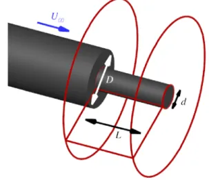
A. Test case and description of the computation The geometry studied consists of an axisymmetric backward facing step similar to the existing experimental S3Ch wind tun-nel configuration studied by Deprés, Reijasse, and Dussauge11and Meliga and Reijasse.46This configuration is composed of a cylinder extended by another cylinder of finite length and smaller diameter, as represented inFig. 1. The characteristic aspect ratios are L
D =1.2
and Dd = 0.4, withL being the length of the smallest cylinder and D and d being the diameters of the largest and smallest cylinder, respectively. This study focuses on the transonic flow regime with a free stream Mach numberM∞equal to 0.7. The Reynolds number
based onD is ReD= 1.2 × 10⁶, and the boundary layer thickness at
the edge of the largest cylinder is δ0
D =0.2. The free-stream dynamic
pressure isq∞=
γ
2M 2
∞P∞≈24, 815 Pa.
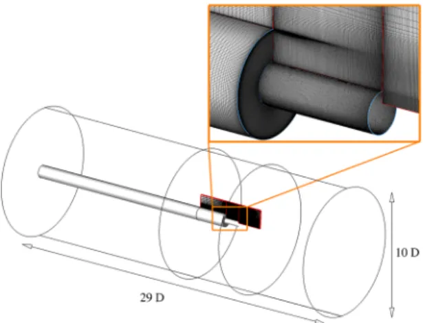
The size of the computational domain represented inFig. 2
together with a close-up of the mesh in the afterbody zone is approximately equal to 29D in the streamwise direction and 10D in the radial direction. The backward facing step beginning at the
end of the larger cylinder is located at x = 174.3D with respect to the inflow, which permits us to obtain the expected values of the integral properties of the boundary layer at the separation point.
FIG. 1. Geometry of the axisymmetric backward facing step with a downstream
cylinder of finite length. L/D = 1.2 andDd =0.4; (→) main direction of the flow with U∞corresponding to the free stream velocity. The red edges define the bounds
FIG. 2. Sizes of the computational domain and close-up view of the mesh in the
separated zone of interest.
The numerical simulation contains four types of boundary conditions:
1. At the inlet: a condition based on a uniform thermodynamic state defined using stagnation quantities.
2. At the wall: a no-slip adiabatic condition.
3. On top of the domain in the normal direction: a nonreflecting boundary condition to avoid spurious wave reflections. 4. At the outlet: a far field condition.
The present analysis is focused on the deep understanding of the flow dynamics in the separated area located in the neighbor-hood of the smallest cylinder (seeFig. 1). This volume of interest containsNi ×Nj×Nk = 171 × 112 × 240 points with a
stream-wise lengthLx = 1.2D, a radial extent Lr = 1.05D, and lθ= 0.4πD and Lθ = 2.5πD for the inner and outer perimeters, respectively. The entire computational domain for this study is made up of a multiblock structured grid containing 12 × 106cells. For the ZDES approach of such a configuration, a grid sensitivity study has already been performed by Deck and Thorigny.8 These authors used three grids containing 5.5, 7, and 8.3 × 10⁶points, showing a convergence for the first- and second-order statistics of the pressure (i.e.,Cp and Cprms). The present grid has been generated taking into account this
previous result. The azimuthal direction, which has formerly been identified as a crucial one beside the streamwise direction for the flow dynamics (see Refs.15and17), is discretized with 240 points, providing a resolution of 1.5○
cell−1. Moreover, the separated areas have been designed to follow the LES requirements in terms of the number of points and cell isotropy. As advised by Simonet al.,23the early stages of the vorticity thickness development are modeled with 15 points.
As represented inFig. 3, this resolution rapidly increases with the mixing layer growth reaching almost 60 points in the radial direction after the middle of the extension (x/D ≈ 0.6). In practice, the grid resolution is not calculated adaptively. The vorticity thick-ness δω = ΔU/ max
y (
∂U
∂y)is plotted with ΔU = U1 −U2, where U1andU2stand for the characteristic streamwise velocities on both
FIG. 3. Streamwise evolution of the number of points clustered in the vorticity
thicknessδω=ΔU/ max
y (
∂U
∂y)withΔU = U1−U2, where U1and U2stand for the characteristic streamwise velocities on both sides of the shear layer.
sides of the shear layer.U1is approximately equal to 237 m s−1, and
U2varies rapidly from −78 m s−1to 5 m s−1. Then, the selected
resolution is related to the aforementioned empirical observation performed by Simonet al.23The number of points clustered in the mixing layer grows rapidly due to the topology that has been adapted to encompass the shear layer. The time-averaged location of the shear has been determined on the basis of a preliminary Reynolds-Averaged Navier-Stokes (RANS) simulation with the same mesh. Such a grid refinement has been shown by Lele47to be sufficient to discretize the layer of fluid linking the vortices inside the mixing layer (i.e., the braids). Indeed, the author used 7 to 8 grid points to resolve the braid region, whereas in the present case, the radial dis-cretization rapidly exceeds 20 points after the separation occurring at the end of the larger cylinder.
Finally, the grid parameters in wall units for x ⩽ 0 in the region treated using ZDES mode 0 (i.e., URANS) are (Δx+, Δr+, Δs+) = (130, 4, 200). The minimum and the maximum values of Δx/D, Δr/D, and Δs/D (where s = θD/2 stands for the grid arc dis-tance) are (Δx/D,Δr/D,Δs/D)min = (0.003, 0.000 15, 0.013 09) and
(Δx/D,Δr/D,Δs/D)max= (0.2, 0.5, 0.1309), respectively. It has to be
noted that the dominant azimuthal wavelength along the streamwise direction found in the following is λθ= πD/2. As a consequence, the dimensionless wavelength of interest is λθ/D ≈ 1.57, which has to be compared to the azimuthal resolution characterized by the grid arc distance that is approximately 100 times lower (i.e., Δs/D ≈0.013) in the mixing layer region. Such a resolution allows us to simulate the upstream attached boundary layer in the RANS mode. The separation is sharp on such a configuration, which means that the integral properties of the upstream boundary layer are the most important to reproduce the flow features. The boundary layer thick-ness at the separation (δ/D = 0.2) is the one predicted by the RANS calculation based on the Spalart-Allmaras turbulence, which is well acknowledged to predict attached flows. Given that the location of the separation is prescribed by the geometry, the integral properties of the upstream boundary layer are of first importance compared to fluctuations. Such a point has been investigated experimentally by Morris and Foss.48These authors have shown that the interaction
between a separated turbulent flow and the fluctuations in an upstream boundary layer can be assumed to be negligible for high Reynolds number flows. This supports the fact that no additional synthetic fluctuations are needed in the incoming boundary layer. In practice, Holmes, Lumley, and Berkooz49suggested the existence of a communication between a mixing layer and a boundary layer for a laminar separation and argued that this is not true for high Reynolds number turbulent boundary layers. As a consequence, a slow deple-tion ofCp is indeed observed, which evidences the strong influence of the recirculation zone on the incoming boundary layer that con-cerns the properties of the mean part of the flow field and not the fluctuating one. Finally, Scharnowskiet al.50performed a numerical
simulation on a similar test case with a longer extension for the same Mach number, namely,M∞= 0.7, using synthetic turbulence
gener-ation and obtained no difference in the recompression process (i.e., the same slow depletion ofCp with the same levels).
B. General description of the numerical setup
The finite-volume solver FLU3M code developed by ONERA51 is used to solve the compressible Navier-Stokes equations on multi-block structured grids. Time integration is performed by means of a second-order accurate backward gear scheme. Spatial discretiza-tion is obtained by a modified AUSM+ scheme proposed by Liou.52 The accuracy of the solver for multiresolution calculations has been assessed in various applications including afterbody flows.8,23,53In these studies, the numerical results are thoroughly compared to the available experimental data including spectral and second-order analyses.
The approach used to model this flow is the Zonal Detached Eddy Simulation (ZDES) proposed by Deck,43,44which belongs to the RANS/LES approaches (see Ref.54for a review). Within ZDES, three different length scale formulations entering the destruction term of the eddy viscosity equation, also called modes, are opti-mized to be employed on three different flow topologies (see Refs.44
and55).
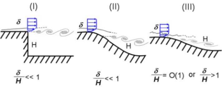
The selection process of the chosen mode is guided by the intrinsic nature of the flow separation (seeFig. 4). The separation locus can be triggered by the geometry (ZDES mode I), a pressure gradient on a smooth surface (ZDES mode II), or the dynamics of an incoming boundary layer (ZDES mode III). This latter mode can be interpreted as a Wall-Modeled Large Eddy Simulation (WMLES) (see Refs.56and57).
FIG. 4. Taxonomy of classical separated flows. I: separation fixed by the geometry,
II: separation induced by a pressure gradient on a curved surface, and III: separa-tion strongly influenced by the dynamics of the incoming boundary layer (adapted from Ref.44).
An example, where all these modes are used in the same cal-culation, is provided in Ref. 58 in the frame of a three-element airfoil.
As a consequence, the present case is treated using ZDES mode I (for x > 0), meaning the area located downstream the separation point is computed with LES, while the area upstream (forx < 0) is solved using the URANS approach (mode 0 of ZDES).
C. Salient features of the flow
As a first glimpse to the global dynamics of the axisym-metric separating/reattaching flow, an overview of the flow topol-ogy is provided in Fig. 5(a) with the visualization of an iso-surface of the normalized Q-criterion (QU2∞/D
2
= 50) colored by the streamwise velocity component coupled with a numerical pseudo-schlieren in a streamwise cut-off plane and at the wall. The dimensionlessQ-criterion is represented in order to evidence the coherent structures of the instantaneous flow.Q is a second-order invariant of the velocity gradient tensor ∇u and is defined as follows: Q =1 2(ΩijΩij−SijSij) = − 1 2 ∂ui ∂xj ∂uj ∂xi >0, (1)
where Sijand Ωijare the symmetric and antisymmetric components
of ∇u, respectively.
It is observed that the coherent structures originating from the edge of the body feature a toroidal shape and rapidly distort to become fully three-dimensional as they are convected down-stream. The numerical pseudo-schlieren allows us to visualize the wide diversity of length scales in the flow and enables us to pic-ture the unsteadiness of the position of the solid reattachment point.Figure 5(b)provides the mean and instantaneous organiza-tion of the flow in a cut-off plane. First, the visualizaorganiza-tion of the isolines ofQU∞2/D
2is coupled with the representation of four main
locations where unsteady phenomena (Kelvin-Helmholtz instability, shear layerflapping motion, impact of coherent structures on the wall, and vortex-shedding) are dominating. The mean streamlines evidence the different recirculation regions that are located around the geometry. Finally,Fig. 5(c)presents the streamwise evolution of the meanCp = p−p∞
q∞ and fluctuating
CpRMS = pqRMS
∞ wall pressure
coefficients. Three characteristic areas can be distinguished. Forx/D ≤0, a slow depletion ofCp is observed, which evidences the strong influence of the recirculation zone on the integral properties of the incoming boundary layer. After the separation,Cp values decrease due to the acceleration of the backflow forx/D ∈ [0, 0.55]. Then, a recompression process dominates the mean pressure field at the wall untilx/D ≈ 1, 2. Concerning the root mean square coefficient of the fluctuating pressureCpRMS, a steady increase is observed in
the rangex/D ∈ [0, 0.85] due to the organized shear layer struc-tures (see Ref.59). This monotonic growth ends with the occur-rence of a plateau in the areax/D ∈ [0.85, 1.1]. Such a behavior is observed for many separated flows (see Refs.60and 61among others). For both quantities, i.e., mean and rms pressure, ZDES reproduces well the experimental distribution shown in Refs. 11
and46.
One can observe fromFig. 5(b)that the present geometry and flow regime involve a solid mean reattachment point that is located at approximatelyx/D = 1.1.
FIG. 5. (a) Isosurfaces of the
normal-ized Q-criterion (QU2 ∞/D
2
= 50) col-ored by the streamwise velocity and numerical pseudo-schlieren (gray scale) in a cut-off plane and on the skin of the emerging cylinder. (b) Figure adapted from Ref.62—Mean (bottom) and instantaneous (top) organization of the flow with mean streamlines (bottom) and isolines ofQU2
∞/D 2
= 50 (top): (1) mixing layer, (2) recirculation zone, (3) mean reattachment point, (4) second recirculation zone, (5) corner flow, and (6) turbulent wake; (I) Kelvin-Helmholtz instabilities 6 ≤ StD ≤8, (II) flapping of the mixing layer 0.07 ≤ StD ≤0.1, (III) coherent structures impingement on the wall StD≈0.6, (IV) vortex-shedding StD ≈0.2. (c) Streamwise evolution of the mean (top) and RMS (bottom) pres-sure coefficient. (—) Zonal Detached Eddy Simulation (ZDES) from Ref. 9 against experimental data from (◇) Ref.11 (kulites), (△) Ref. 11 (steady tabs), and (•) Ref.46.
The literature related to axisymmetric backward facing step flows provides a background knowledge for the hereby dynamics analysis. Four normalized frequencies based on the greatest diam-eterD were identified to be responsible for the most energetic loads applied on the afterbody. The areas where each frequency is domi-nant were located and associated with coherent structure scales. For instance, Deprés, Reijasse, and Dussauge11 related the large scale
vortices in the wake region toStD= 0.2. Weisset al.9evidenced the
absolute nature of them = 1 antisymmetric mode mainly responsi-ble for the side loads and associated withStD= 0.2 by means of a
local linear stability analysis. Furthermore, these latter authors con-firmed the helical behavior of the absolute instability, as suggested by previous studies.14,17
Huerre and Rossi63 carried out a stability analysis on a free shear layer and derived an expression for the evolution of the fre-quencyf in the streamwise direction as a function of the vorticity thickness of the shear layer (denoted δω).
These authors thus put forward that the Kelvin-Helmholtz instability, which occurs in the mixing layer originating from the separation point at the edge of the cylinder of diame-ter D, is characterized by the range of normalized frequencies 6 <StD<8.
The frequency range around StD = 0.07 was linked to the
mixing layer flapping motion, as exposed by Driver, Seegmiller, and Marvin.12 Finally, it was evidenced by Deck and Thorigny8 that the reattaching point on the emerging cylinder oscillates at StD= 0.6.
III. SPATIAL ORGANIZATION OF THE FLUCTUATING PRESSURE FIELD
This section aims at characterizing the spatial organization of the fluctuating pressure field around the backward facing step of finite length (Fig. 1). For that purpose, the instantaneous static pres-sure field within the computational volume shown inFig. 1 was sampled through the ZDES numerical simulation.
The domain located behind the short cylinder in the wake is not sampled. This choice is motivated by the investigation of Deck and Thorigny,8 which concerned the same geometrical configura-tion as the present one with a major difference, namely, the inclu-sion of a supersonic jet located at the base of the short cylinder to represent the effect of a nozzle. In this case, the supersonic jet issu-ing from the nozzle is actissu-ing as a wall for the surroundissu-ing flow. Thus, in this former study, there is no secondary recirculation bub-ble in the wake downstream the short cylinder as in the present case. Comparing numerous relevant quantities for these two configura-tions (i.e., with and without jet), such as the streamwise evolution of the mean and fluctuating pressure coefficients or the character-istic frequencies resulting from spectral analyses (e.g., single-point and two-point spectra), no significant differences were observed. These results are fully in line with the experimental investigation by Deprés, Reijasse, and Dussauge11on this transonic axisymmetric step flow. Finally, this would suggest that the secondary recircula-tion is not of first importance in the flow dynamics, given thea priori weak interactions with the primary recirculation zone.
The time step of the simulation is equal to 2 μs. However, sam-pling is not performed at every time step, which would correspond tofsamp= 500 kHz. In practice, the fluctuating quantities are stored
every 5 time steps, leading to a sampling frequency of 100 kHz. This choice is supported by the fact that no energy is observed in the spec-tra anymore for frequencies higher than 100 kHz allowing us to limit the data storage. Thus, the numerical sampling time isTacqU∞/D
= 476 (i.e.,Tacq= 0.2 s), and the sampling rate isfsamp= 100 kHz in
order to avoid any aliasing problem. The resulting database is com-posed of 20 000 snapshots with Δt U∞/D = 0.024 representing 2 TB
of data storage.
As discussed in Ref.64, there is a contradictory aspect between the needs for statistics and the constraints imposed by computa-tional fluid dynamics (CFD). Indeed, to perform a statistical analysis in good conditions, the signal has to be well sampled on a suffi-cient duration because the spectral information needs to be averaged on many blocks to be statistically converged. In practice, unsteady signals issued from CFD are most often oversampled on a short duration [due to high central processing unit (CPU) cost]. Thus, a compromise has been found between the number of averaged blocks and the frequency resolution. The useful unsteady calcula-tion ofT ⋅ U∞/H = 1580, which means that 200 ms of physical time
has been simulated, is quite significant in terms of the CPU time consumed. Considering the fact that the main frequency of inter-est is hereStD= 0.2 corresponding to 474 Hz (i.e., almost 0.002 s),
we gather 100 periods of the shedding phenomenon. This sampling is already expensive. The time step was equal to 2 μs, providing a minimal frequency that can be captured of 5 Hz. Considering a res-olution for the spectrum of 60 Hz, we manage to average the spectral information over 23 blocks with a 50%-overlap using a Hamming window.
A Discrete Fourier Transform (DFT) is applied to this unsteady dataset. Then, the fluctuating pressure field distribution is investi-gated looking at the three-dimensional spectral content in the fre-quency and wavelength spaces. Another approach, namely, a two-point correlation analysis as performed by Fuchs, Mercker, and Michel,15also reveals the spatial organization of the fluctuating field. A. Energy distribution in Fourier space
First, the frequency content of the separated region is inves-tigated by means of a temporal discrete Fourier transform. The temporal discrete Fourier fransform provides Fourier modesX( f ) defined on a given frequency range. The spectral investigations are carried out on a frequency window ranging from 5 Hz to 100 kHz by steps of Δf = 60 Hz (ΔStD∼0.025). At each location in the com-putational volume (seeFig. 1), DFT is applied in order to compute the Power Spectral Density (PSD) of the local fluctuating static pres-surep′(x, y, z, t) = p(x, y, z, t) − p(x, y, z). The one-sided PSD is here
denoted byGp′(f ) and reads
σ2= ∫ ∞ 0 Gp ′(f )df =∫ ∞ −∞ f ⋅ Gp′(f )d[log( f )], (2) where σ is the standard deviation of the input signal. Gp′(f ) indicates
how power is distributed in the frequency domain. Once the PSD spectrum has been computed at each location, the local maximum value forGp′(f ) and the corresponding frequency f (max[Gp′(f )])
are extracted. Each leads to a set ofNi×Nj×Nkvalues averaged
FIG. 6. Contours of the power spectral density local maximum max[Gp′(f )] in (Pa2 Hz−1) (top, left) against contours of the local maximum normalized PSD
max[fGp′(f )/σ2] (bottom, left) in plane (x/D, z/D). Contours of the correspond-ing Strouhal numbers: (top, right) StD(max[Gp′(f )]) against StD(max[fGp′(f )/σ2]) (bottom, right).
over the azimuth, which is plotted inFig. 6. The top two plots present the contours of max[Gp′(f )] (gray scale) and StD(max[Gp′(f )])
(col-ored scale), the normalized frequencyfD/U∞based on the
diam-eterD and the free stream velocity U∞. The spectra are averaged
in the homogeneous azimuthal direction. Thus, the graphic rep-resentation is reduced to the plane (x, z). In order to combine different levels of information, the contours of max[fGp′(f )/σ2]
(gray scale) andStD(max[fGp′(f )/σ2]) (colored scale) are depicted
in Fig. 6 (bottom). While Gp′(f ) provides the energetic level of
each frequency,fGp′(f )/σ2returns the relative contribution of each
frequency with respect to the total signal characterized by σ2[see Eq.(2)].
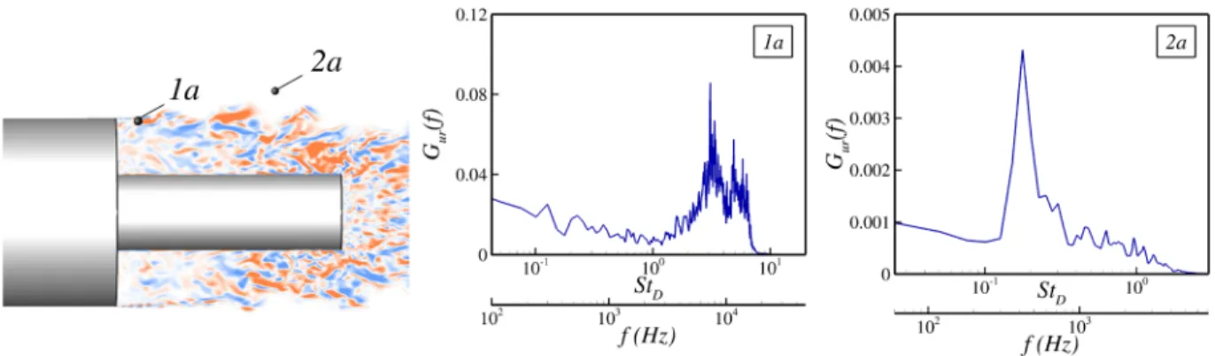
In order to illustrate the representativeness of the PSD peaks selected to plot the two-dimensional maps of the PSD maxima, single-point spectra for the radial velocity ur are shown for two
locations in Fig. 7. The definition ofGur(f ) is similar to that of
Gp′(f ) in Eq.(2). The numerical sensors are located inside and
out-side the mixing layer. Despite the two different frequency ranges that can be noted, in both cases, a broadband spectrum is observed along with a very prominent peak, allowing an unambiguous selec-tion of the maximum. The frequency content evolves a lot from point 1a to point 2a. Point 1a is located inside the mixing layer and exhibits two harmonics, namely,StD= 3 and 6 that correspond to
typical high frequencies related to the vortex pairing phenomenon. The dimensionless frequencyStD= 0.18 that is characteristic of the
vortex shedding phenomenon can be distinguished. However, the shedding at point 1a is clearly overwhelmed by the shear layer pro-cess and is far less prominent than at point 2a, which shows a clear peak atStD= 0.18. This physical interpretation is supported byFig. 6
(right).
The spectral map inFig. 6(top, left) indicates that the fluctu-ations with the highest levels are located on the second half of the emerging cylinder (0.55 ≤x/D ≤ 1.0), within the recirculation bub-ble (z/D ≤ 0.5). Besides, traces of intense fluctuations are captured
FIG. 7. Contour map of the streamwise vorticity sign (blue for negative and orange for positive) along the location of two sensors (left) used to plot single-point spectra at two
characteristic locations inside (middle) and outside the mixing layer (right).
in the area 0 ≤x/D ≤ 0.4 and z/D = 0.5. The corresponding Strouhal numbers in this latter region are of the order of those expected in an early shear layer stage (StD≥3.0), as shown inFig. 6(top, right). The most significant unsteady feature of the flow appears to be related to the dimensionless frequencyStD= 0.18. The selected locus of this
frequency is confined in a stripe-shaped area, which lies from the emerging cylinder wall up to the free stream, passing through the mixing layer. This implies a very robust and dominant local dynam-ics that seems to propagate in the radial direction. Such a result corroborates those of Weisset al.9who carried out a linear stabil-ity analysis on the present axisymmetric flow and put forward the absolutely unstable nature of the area 0.35 ≤x/D ≤ 0.75. This area is represented in gray dashed lines inFig. 6. Forx/D ≥ 1.0, the wake dynamics feedback occurring atStD= 0.18 andStD∼0.6 can be
inter-preted as the signature of the classical vortex-shedding phenomenon found in the wake region.16,65
ConsideringFig. 6(bottom, left), a beam of high max[fGp′(f )/σ2]
values is observed in the mixing layer. This area highlights that the major part of the fluctuating energy arises from the Kelvin-Helmholtz instabilities. The corresponding Strouhal number map [Fig. 6 (bottom, right)] clearly depicts a linear spreading of the most amplified frequency, which reflects the behavior of a free mixing layer. In the second part of the cylinder extension, the inner part of the impinging shear layer presents a blurred distri-bution of the spectral content. In particular, the symmetry in the shear layer beam is broken at x/D ∼ 0.3 and z/D ∼ −0.3 with a wider frequency range dominated by the Strouhal number value StD≥1.0. Such a breakdown in the symmetry may be the conse-quence of the intermittency of the reattachment point as shown by Weiss and Deck,53 resulting in an upstream and downstream convection of the impinging Kelvin-Helmholtz structures (see Ref.59).
On top of this major source of turbulence, secondary patterns whose limits are indicated by two vertical dashed lines can be dis-tinguished in the spectral map inFig. 6 (bottom, left): one close to the wall in the absolutely unstable zone and two located in the outer part of the Kelvin-Helmholtz instability. According toFig. 6
(bottom, right), those patterns correspond to the aforementioned StD= 0.18 dynamics. This suggests that the first half of the
recircu-lation region is mainly driven by mechanisms of Kelvin-Helmholtz
type, whereas the far field dynamics is led by vortex-shedding periodicity.
It is distinguished an area withStD∼0.07 close to the separa-tion point, spreading on theouter part of the shear layer. Such low frequency dynamics are ascribed to the flapping motion of the mix-ing layer.12Finally, the highStDregion in the far field (aroundz/D
∼ −1 andx/D ∼ 0.9) may be associated with turbulent noise radiating from the K-H instabilities.
B. Azimuthal coherence distribution
As previously done by Fuchs, Mercker, and Michel15 behind a circular disk, a modal decomposition in the azimuthal direction has been performed in order to quantify the correlation between two time signals in space. In the cylindrical coordinate system (r, θ, x), let ϵ1(r1, θ1,x1,t) be the signal at sensor 1, which will be considered
as the reference input. Let ϵ2(r2, θ2,x2,t) be the second signal to be
compared. Finally, a measure of the correlation between both signals by means of the coherence function is given by
C( f , r1, Δr, θ1, Δθ, x1, Δx) =
G12(f , r1, Δr, θ1, Δθ, x1, Δx)
√
G1(f , r1, θ1,x1)G2(f , r2, θ2,x2) = (Cr+jCi)(f , r1, Δr, θ1, Δθ, x1, Δx), (3)
whereG1 andG2 are the autospectrum of each signal andG12 is
the corresponding interspectrum. Δr, Δθ, and Δx define the radial, azimuthal, and axial relative positions, respectively, between the two sensors. Here, the azimuthal direction is investigated; thus, the com-putation of C reduces to pairs of sensors with r1 = r2 = r and
x1=x2=x. Larchevêque et al.66emphasized that prior to physical
interpretations, one should determine the threshold beyond which the coherence γ becomes statistically significant. Such a threshold denoted that γ99%depends on several parameters detailed in the
lit-erature.67On the basis of a Fisher law with a confidence interval of 99%, a level of γ2stands for an effective correlation if γ > γ299%with:
γ299% ≳1 − 10
(−4
ndof)according to Koopmans.67In the definition of
γ299%,ndof = 1811nbcorresponds to Welch’s degrees of freedom (see
Ref.68) withnbbeing the number of blocks over which the spectra
are averaged. For the present case, the estimation of such a threshold returns γ > γ299%∼0.40, where γ = ∥Cr+jCi∥.
FIG. 8. (Left) Evolution of the real part of the coherence
function for the first four azimuthal modes for StD= 0.18
along the streamwise direction at the wall. (Right) Spectral map (StD, x/D) of the first azimuthal pressure mode Cr,m=1
at the wall (r/R = 0.4, with R being the radius of the greatest cylinder).
At this point, it is important to be reminded of two major assumptions about the correlation function:
● Azimuthal homogeneity: C does not depend on the azimuthal position of the reference sensor (sensor 1) but only depends on the relative offset between the signals (Δθ). ● Azimuthal isotropy: statistically, the fluctuations should equally propagate in the positive and negative sense along the azimuthal direction. This assumption leads toCi= 0.
Finally, the resultingCrfunction is 2π-periodic with respect to
Δθ and can be expressed, thanks to a Fourier transform in azimuthal modes. In the present case,
Cr(f , Δθ) =
∞
∑
m=0
Cr,m(f ) cos(mΔθ), (4)
whereCr ,m(f ) denotes the relative contribution of mode m to the
fluctuating energy at frequencyf since ∑
mCr ,m= 1.
On the experimental side, Deprés, Reijasse, and Dussauge11 carried out a similar decomposition. In Ref.9, the study of the spatial organization of the energy for a given modem was performed at the wall and not in the flow field as in the present work. By performing a coherence analysis in planes normal to the flow at three stations (x/D = 0, 0.12, and 0.55) on the wall of the emerging cylinder, the authors put forward that the highest levels of coherence forStD∼0.2 occur for an interval Δθ = π between the pressure sensors. They deduced that this frequency is driven by the azimuthal modem = 1.
In the numerical simulation here, this assumption is verified inFig. 8(left) in which the first azimuthal mode clearly dominates
atStD= 0.18 along thex/D direction with a maximum value of the
coherence valueCr ,m=1= 0.8 reached atx/D = 0.5.Figure 8(right)
shows the distribution at the wall of the real part of the coherence function for the azimuthal modem = 1. The map illustrates that on the first half of the separated flow, the dynamics involving two dia-metrically opposite points (Δθ = π) is mainly governed by the shear layer flapping motion (StD∼0.07), while the second half exhibits high correlations aroundStD∼0.2. It is worth noting the coexis-tence of both frequencies in the area 0.3 ≤x/D ≤ 0.75, followed by the drop ofCr ,m=1forStD∼0.07 to the benefit ofStD= 0.18. This
suggests that the absolutely unstable zone may confine the effect of the flapping motion in the upstream region form = 1.
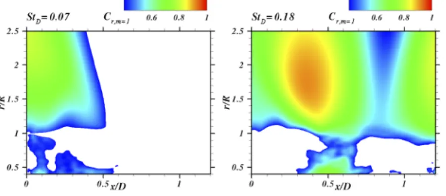
In order to elucidate the origins of theCr ,m=1distribution at
the wall, a coherence analysis in the radial direction has been per-formed for the main frequencies inFig. 9. This latter depicts the spectral map (x/D, r/R) of the first azimuthal mode for StD= 0.07 and
StD= 0.18. As inFig. 8(right), only the first half of the separated
flow features high correlation levels atStD= 0.07. Nevertheless, an
area of high correlation is found in the range 0 ≤x/D ≤ 0.5 above the mixing layer (r/R ∼ 1), where the flow dynamics is not disturbed by any turbulent fluctuations. It is also worth reporting some significant coherence areas underneath the mixing layer. This suggests that the flapping dynamics constitutes a robust feature of the turbulent shear layer and significantly affects the organization of the recirculation area.
High correlation levels in the mixing layer also occur in the interval 0.3 ≤x/D ≤ 0.8 for StD= 0.18, as shown inFig. 9(right).
One should remark that the specific positionx/D ∼ 0.3 corresponds to the locus where the Kelvin-Helmholtz fluctuations become less
FIG. 9. Spectral map of the first azimuthal pressure mode
Cr,m=1along the streamwise (x/D) and radial (r/R) directions
intense according toFig. 6(left). Finally, by the end of the emerging cylinder, the feedback of the wake vortex-shedding is captured as it was mentioned previously.
In this subsection, it has been put forward that the unsteady dynamics is governed by the first azimuthal mode m = 1, which implies that fluctuations at two diametrically opposed points are paired in time. Then, the spatial distribution of the most excited Strouhal numbers is typical of the flapping motion of the mixing layer (StD = 0.07). This dynamics dominates in the first part of
the emergence before being overwhelmed by the vortex-shedding phenomenon (StD = 0.18). The dynamics of the flow phenomena
related to these two frequencies appears to be stronger in the free stream.
More globally, the three-dimensional fluctuating field has been characterized both in the Fourier space and in terms of azimuthal coherence. This analysis provides a detailed profile of the unsteady axisymmetric backward facing step flow. Yet, a further insight is required in order to shed light on the three-dimensional spa-tial organization of each characteristic frequency of the fluctu-ating field. Practically, such an analysis is usually performed by decomposing the flow structures into modes. In this study, the Fourier mode decomposition method is used. Results are discussed in Sec.IVin which a comparison with the recent dynamic mode decomposition method is also performed to cross-check the first analysis.
IV. MODAL DECOMPOSITION
OF THE THREE-DIMENSIONAL PRESSURE FIELD A. Fourier modes
It is reminded that the temporal discrete Fourier transform provides Fourier modesX( f ) defined on a given frequency range and that the spectral investigations are carried out on a frequency window ranging from 5 Hz to 100 kHz by steps of Δf = 60 Hz (ΔStD∼0.025).
The previous analysis focused on the power spectral density Gp′(f ) of each Fourier mode, i.e., the square modulus of X( f ) over
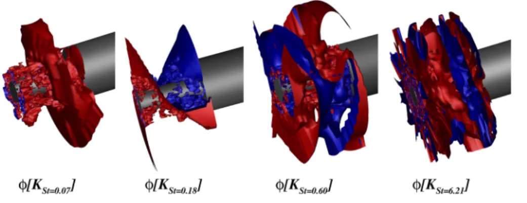
the integration period for each frequency band Δf. In this section, each Fourier mode is considered in its complex form at each point in the computational volume (shown inFig. 1). The complex Fourier modes associated with the four characteristic frequencies identified in the preliminary investigations [StD = 0.07, 0.18, 0.60, and 6.21
(±0.025)] were extracted. The specific value of the dimensionless fre-quencyStD= 6.21 has been selected to illustrate the shape of the
mode related to the characteristic frequency observed in the early stages of the shear layer. This value decreases downstream in the mixing layer far from the separation, as mentioned in Ref.53. In the early stages of the mixing layer, the characteristic high frequen-cies are ranging fromStD= 5 toStD= 8. Both the Fourier and DMD
modes have similar shapes in this range. Modes are represented for each characteristic frequency range, namely,StD= 0.07 for the
flap-ping phenomenon,StD= 0.18 for the shedding phenomenon,StD
= 0.6 for the oscillation of the reattachment point of the recirculation bubble along the extension, andStD= 6.21 for the K-H instability.
Weisset al.9 showed, thanks to a linear stability analysis, that the axisymmetric body dynamics is led by a significant unstable area centered around x/D ≈ 0.55, suggesting a global instability
mechanism. Let us be reminded that in that case, the flow can behave as an oscillator and imposes its own dynamics. Self-sustained oscil-lations are observed, which are characterized by a well-defined fre-quency f0 (or wavelength λ0). This behavior is clearly educed in
Fig. 8showing the spatial distribution of its energy, and the anti-symmetric nature of the corresponding mode has been investigated by the azimuthal Fourier transform of the interspectrum of pressure fluctuations at frequencyStD= 0.18 (Fig. 9).
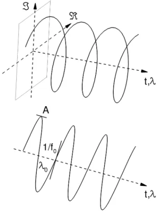
As an additional way to investigate this major property of the flow, one can also consider directly the spatial distribution of the local single-point time Fourier transform. As a preliminary exam-ple, let us consider the complex exponential mode of pure harmonic behavior, i.e., characterized by its frequencyf0(or wavelength λ0),
Ae2jπf0t(orAe2jπλ0λ) that has a constant modulusA.
Figure 10reminds that there are different ways of consider-ing such a signal by either its real R(●) and imaginary part I(●) or its amplitude and phase ϕ = A tan(R(●)I(●)). To get further insight into the spatial organization of the intrinsic dynamics of the flow, the complex Fourier transformX( f ) of the fluctuating pressure field p′(t) is analyzed.
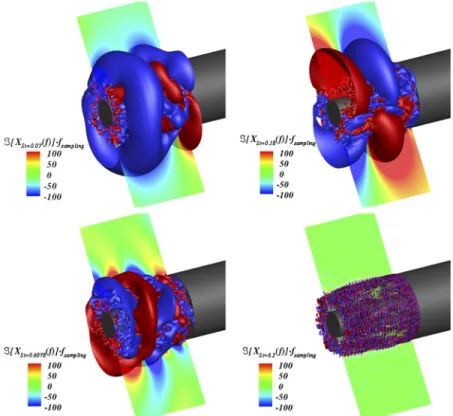
First,Fig. 11displays the imaginary part of the Fourier mode (I(XStd=cst(f ))) on each grid point for a set of selected frequencies of interest. Contours are normalized by the sampling frequencyfsamp
to directly obtain a data representation in a physical unit, i.e., Pas-cals (Pa). The selected computational volume allows us to extract
FIG. 10. Different depictions of the modelAe2jπf0t(orAe2jπ λ λ0).
FIG. 11. Contours ofI(X(f )) ⋅ fsamp(Pa) and isosurfaces I(X(f )) ⋅ fsamp=200 (red) andI(X(f )) ⋅ fsamp= −200
(blue) of the Fourier modes associated with (from top left to bottom right) StD= 0.07, StD= 0.18, StD= 0.60, and StD
= 6.21 (the flow goes from right to left).
half of a wavelength in the streamwise direction for this specific Strouhal number. As expected, considering the spatial distribution of the observed patterns, the wavelength decreases as the Strouhal number increases. Besides, contours of I[XStD=cst(f )] at StD= 0.18
clearly exhibit a sequence of diametrically opposed positive and neg-ative patterns with alternating orientation in the direction transverse to the flow. One can note that both experimentally and numeri-cally, the flow is likely to adopt one single orientation due to local perturbations (surface roughness and numerical methods).
In contrast to the fully antisymmetric behavior observed at StD= 0.18, a large axisymmetric pattern located on the second half of
the emerging cylinder is evidenced atStD= 0.07. Such a difference
is consistent with the results of Deck and Thorigny8who unveiled that the shear layer flapping motion aroundStD= 0.07 is associated
with the azimuthal modem = 0, while the vortex shedding is related to the antisymmetric modem = 1. Then, two diametrically opposed zones are observed close to the separation edge. This spatial distri-bution corroborates the results of Sec.III B. In this section, the area 0 ≤x/D < 0.55 is characterized by a high coherence level for the first azimuthal mode (seeFig. 9), which rapidly falls to low levels ofCr
forx/D ≥ 0.55.
The spatial distribution of the Fourier mode related to StD
= 0.60 is similar to that ofStD = 0.18 with a shorter streamwise
wavelength. One should note that for this frequency range, the pres-sure contours are extended in the radial direction and slightly tilted downstream. This feature may be related to the acoustic propagation and the tilting to the advection effect.66
The isosurfaces of I[X( f )] ⋅ fsamp = ±200 (Pa) at StD
= 6.21 inFig. 11(bottom, right) clearly show the presence of toroidal
structures that are convected along the direction of the shear layer and remain well organized as a sequence of alternated positive and negative high fluctuating pressure zones. Such a distribution is characteristic of the Kelvin-Helmholtz convective instabilities, as discussed by Huerre and Rossi.63
To further investigate the dynamics associated with a given fre-quencyStcs, the focus is put on the inverse Fourier Transform of the
pressure Fourier mode. Indeed, the inverse discrete Fourier trans-form states that the initial discrete pressure signalp′(t
i) (i = 1, . . ., N)
can be rebuilt from all the Fourier modes (X( fk))f
k=Nkfsamp,[k=0,...,N−1].
Due to the Hermitian symmetry of the discrete Fourier trans-formX( fk) =X∗(fN −k), the reconstructed fluctuating pressure field
p′ r(ti) is real-valued, p′ r(ti) = 1 N N−1 ∑ k=0 X( fk) ⋅e2πj k Nti. (5)
Then, following this reconstruction step, only one mode for each characteristic frequency of the flow dynamics is selected. Let Stcs be the characteristic selected frequency, andp′r(ti)∣Stk=Stcs
=X( fk)∣Stk=Stcs⋅e
2πjk
Nti∣Stk=Stcs is complex-valued, whilep′
r(ti) defined
by all modes [see Eq.(5)] is real-valued.
The physical interpretation of I(X( fk)∣Stk=Stcs⋅e
2πjk Nti∣Stk=Stcs
)is not commonly used, but, in practice, this quantity is simply related to the time derivative ofp′(t
i),69which is relevant to evidence a large
scale unsteady process.
To complete the representation of the mode, both the real and imaginary parts of the DMD modes as well as the corresponding phase are plotted (seeFigs. 12,13and14).
FIG. 12. DMD isosurfaces and contours
ofI(Kj): StD≃0.07, StD≃0.18, StD
≃0.60, and StD≃6.21 (the flow goes from right to left).
FIG. 13. DMD isosurfaces and contours
ofR(Kj): StD≃0.07, StD≃0.18, StD ≃0.60, and StD≃6.21 (the flow goes from right to left).
Figure 15shows four snapshots of the inverse Fourier mode dynamics associated with StD = 0.18 with a time interval Δt
=T/6|St =0.18between each other so that the half of a period is
repro-duced. Organization at t = T0 has been discussed above and is
consistent with the conclusion of the spectral study in the wave number space, which evidenced the dominance of λθ= πD/2. The snapshot at timeT0 +T/6|St =0.18illustrates the convection of the
large scale pairs at the extremity of the emerging cylinder toward the
FIG. 14. DMD isosurfaces and contours
ofϕ(Kj): StD≃0.07, StD≃0.18, StD
≃0.60, and StD≃6.21 (the flow goes from right to left).
FIG. 15. Visualization of the computed inverse Fourier
mode dynamics (imaginary part) associated with StD= 0.18.
The values of the two isosurfaces areI(X(f )) ⋅ fsamp
= 200 (red) andI(X(f )) ⋅ fsamp = −200 (blue). Each picture isΔt = T/6|St =0.18apart from the top left to bottom
right (the flow goes from right to left).
wake region. This is coupled with a slight convection downstream close toD/4 and a growth in size of the upstream negative fluctuat-ing pressure pattern (represented in blue). SnapshotT0+ 2T/6|St =0.18
depicts the appearance of an extra pair of structures close to the separation edge while the initial ones keep convecting downstream. The last snapshot inFig. 15exhibits a switch in the organization of the first snapshot since the exponential term in Eq.(5)provides the periodic aspect of the dynamics and bears the intrinsic pulsation of StD= 0.18.
It is remarked that the most amplified pressure patterns (snap-shotsT0and T0+T/2|St =0.18) occur at specific locations alongx.
The first one is located in the absolutely unstable area (0.35 ≤x/D ≤0.75) identified by Weisset al.,9 while the second one is located by the edge of the emergence (0.75 ≤x/D ≤ 1.2). This suggests that the dynamics in the radial direction is mostly driven by the intrin-sic pulsations of the absolutely unstable region. Periodically, large scale coherent structures emerge from that region. As they convect downstream and reach the edge of the small cylinder, they are likely to induce large scale vortices, rotating in the streamwise plane, due to the radial pressure gradients and constitute the von Kármán alley in the wake region.
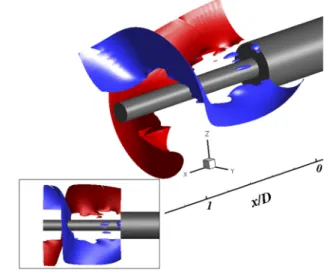
In this paragraph, the spatial distribution of the Fourier mode is investigated by considering the phase ϕ(X( f )) =atan[I(X( f ))/R(X( f ))], which, therefore, provides the location of the Fourier mode in the complex plane. The regions of positive and negative values for the phase ϕ(X( f )) exhibit a helical shape for StD = 0.18. This is emphasized in Fig. 16 with the isosurfaces
ϕ(X( f )) = ±0.02 that bound the two different areas. Direction x in the figure was stretched for graphical purposes. Such a spatial structure of the pressure fluctuations related to the vortex-shedding is consistent with the experimental observations of Taneda14and
FIG. 16. Isosurfaces ϕ(X(f )) = ±0.02 of the phase ϕ(X(f )) = atan(I(X(f ))/R(X(f ))) of the Fourier mode associated with StD
Berger, Scholz, and Schumm17who put forward the assumption that the flow past a sphere might adopt a helical organization. Monke-witz16showed that the preferred instability mode in the axisymmet-ric wake is a spiral, which was explicitly evidenced by Weickgenannt and Monkewitz19 on an axisymmetric bluff body wake atReD= 3
×104with a representation of the phase-locked velocity. To the best of the authors’ knowledge, this helical mode is highlighted for the first time in physical space, thanks to a Fourier analysis of the fully three-dimensional fluctuating field. Besides, the coexistence of abso-lute helical (m = 1) unstable global modes within the recirculation region and convectively unstable shear layer modes corroborates the results of Sandberg and Fasel10on supersonic axisymmetric wakes.
Since the large scale helical structure is captured at the early sep-aration stage of the flow, it suggests that the spiral organization exposed by Monkewitz16derives from the convergence of the helix, as it convects downstream, toward a location on the axisymmetric axis. The data provided in this study do not allow us to confirm such an assumption since the computational volume of acquisition is restricted to the recirculation area. In addition, the presence of the emerging cylinder may certainly affect the evolution of the spiral radius compared to the case of a single axisymmetric bluff-body.
For bluff-body flows, the analogy between a low-Reynolds (laminar and incompressible) configuration, such as the cylin-der plate or sphere case,6,20,70–72 and higher Reynolds number
(and high subsonicM∞ = 0.7) is hardly comparable. Indeed, the
flow around a sphere at Re = 300 is the seat of a self-sustained instability around the Strouhal number of 0.135. This dynamics generates vortex-shedding formed by coherent structures such as hairpins. The higher Reynolds number dynamics has different char-acteristics. Although a fully turbulent flow may also be the site of a global instability (dynamics temporally self-sustained), like its laminar counterpart (see Ref.9), the spatial development of these instabilities is generally very different. The reason is that there are also highly unstable convective instabilities (and sensitive to differ-ent environmdiffer-ental forcings) at high Reynolds numbers that interact and blend with the global instabilities generating complex structures formed by an aggregate of smaller structures. The helical structure described in this paper is obviously not a coherent structure as can be the hairpin at low Reynolds numbers but rather a cluster of spatiotemporally correlated structures. The pre-existence of coher-ent structures upstream can further complicate the spatiotemporal dynamics.
The rapid phase variation of the azimuthal Fourier modem = 1 observed at x/D ≈ 0.9 in Fig. 16 is indeed quite brutal because it corresponds to a sudden change in dynamics. The beginning of the emergence (x/D < 0.5) corresponds to the development of the vortex structures attached to the mean shear-layer and driven mainly by the mean local vorticity thickness δω(x). Around x/D ∼ 0.5, the structures attached to the mean shear-layer are shed-ded, the coherent structures no longer follow the mean shear-line, and this is the vortex-shedding phenomenon. The global motion is then mainly helical (with an azimuthal wave numberm = 1, see Ref. 9). On the other hand, the existence of an absolute (global) instability in the zone9 of an azimuthal wave numberm = 1 rep-resents the presence of a helical dynamics, which drives the flow downstream.
As for the validity of a linear stability analysis for a turbulent flow, it has indeed been carried out for a long time with sometimes
a real success but without real theoretical justification. Recent stud-ies are beginning to better lay the theoretical framework of such an analysis.73–75
In the study by Statnikov, Meinke, and Schröder,30 a cross-flapping motion of the shear layer is observed atStD≃0.2, triggered by antisymmetric vortex shedding. The present results first intro-duced in Ref.26show the same thing. The main differences lie in the interpretation of the dynamics of the antisymmetric character. In both simulations, there are hairpins, lambda vortices, stripes, and structures on the scales of the order of the vorticity thickness of the shear profile. These structures do not play a direct role in the anti-symmetric dynamics atStD≃0.2. A major difference lies in the jet of the nozzle, which is included in the work of Statnikov, Meinke, and Schröder30and not in the present study. Taking this jet into account can significantly alter the overall dynamics of the wake and could lead to different conclusions. However, it is important to note that the presence of the jet does not alter the existence of aStD≃0.2 dynamics that originates in an absolutely unstable zone around the extension and not in the near wake (Weisset al.9). The near wake, which is of convective (and not absolute) nature, is then forced by this temporally self-sustaining dynamics and develops convec-tively unstable instabilities. The latter are strongly influenced by the local topology of the flow and, therefore, by the presence or absence of the jet.
As it was mentioned above, the helix seems to feature an anti-clockwise oriented rotation when facing the flow. Although here the helix pitch is not constant alongx due to the stretching of the x direc-tion, it can be measured that the isosurface ϕ(X( f )) = 0.02 covers an angle π across a distance lπ∼0.9D leading to an approximated pitch α ∼ 0.29D (m rad−1). The complete rotation is thus expected to be performed for l2π ∼1.8D. This is of the order of the abso-lute wavelength λ0from Weisset al.9who derived the streamwise
evolution of λ0by means of a linear stability analysis and obtained
λ0= 2.05D in the absolutely unstable region. Even though
Weick-genannt and Monkewitz19investigated the axisymmetric bluff body wake in the Reynolds number range 3 × 10³≤ReD≤5 × 10⁴, the authors did not report the effect ofReD on the geometrical
char-acteristics of the spiral. Yet, from the downstream evolution of the phase-locked velocity ⟨Vx⟩/V∞,
19the approximated spiral pitch is
αbluff-body ∼0.64D (m rad−1) at ReD = 3 × 10⁴. This conjectures
that the higher the Reynolds number, the lower the pitch and the more spin the spiral gains. Armalyet al.7experimentally evidenced on a three-dimensional backward facing step that the length of the recirculation bubble decays as the Reynolds number increases. This would support the previous assumption that the helical dynam-ics is compressed to a smaller volume as the reattaching length decreases.
To conclude, the spatial organization associated with the main frequencies identified in Sec. III, namely, StD has been
evidenced. The analysis of the imaginary part of the Fourier modes highlighted the antisymmetric nature of the fluctuating pressure 3D distribution associated with StD = 0.18 as opposed
to axisymmetric structures for StD = 0.07. A temporal
recon-struction of the Fourier mode associated with StD = 0.18 has
been performed in order to investigate the radial dynamics of the vortex-shedding phenomenon. Finally, the visualization of the phase of X( f )|St =0.18 puts forward the helical nature of that
B. Dynamic modes
In the diversity of modal decomposition methods, the Dynamic Mode Decomposition (DMD) derived by Rowley et al.76 and Schmid77 has been used in this section with the view to support the results of Sec.IV A. This method relies on the spectral analysis of a linear operator called the Koopman operator.76Each dynamic mode is characterized by its own frequency. As such, this method is a well-adapted tool to compare with the above results. Chen, Tu, and Rowley78 have mathematically shown that DMD on mean-subtracted input data is equivalent to the temporal discrete Fourier transform. The aim of this section is to apply the dynamic mode decomposition on such an input data contest with the view to cross-check the spatial distribution that has been derived above with an alternative approach.
The main purpose of this study is to show that the nonlinear dynamics of a flow around an axisymmetric backward-facing step with a downstream cylinder has a large-scale helical structure as well as a hierarchy of structures at intermediate scales. To the best of the authors’ knowledge, the illustration of such a result by two different methods constitutes a novelty.
Concerning the equivalence between the temporal discrete Fourier transform and the DMD, there are several works giving a framework to this equivalence. Historically, Rowleyet al.76and Schmid77 proposed the DMD that has the advantage to be a fre-quency modal decomposition easily accessible. SeeAppendixfor a detailed description of this method. The advantage of the DMD, relative to other frequency decompositions such as Fourier decom-position, is to better grasp the real physical mechanisms, in par-ticular, for transient or nonequilibrium phenomena. The DMD can be used with both experimental and numerical data. The main constraint is to have access to sufficiently time-resolved data. One important difference between, for example, another decomposition like POD and the DMD algorithm is that the mean is not first subtracted for DMD. This is important to note that it can be shown that subtracting the mean before applying DMD gives results identical to a temporal discrete Fourier trans-form (see Ref. 78), if the equation yk+1 = Ayk, k = 1, . . ., m
(see theAppendix) is satisfied exactly (e.g., if the firstm snapshots are linearly independent). Generally, this equivalence is obtained when the flow is statistically stationary.
In our case, although the flow is fully turbulent, the latter is massively separated, whicha priori does not allow us to be certain to be “statistically stationary.” Indeed, there is, in particular, a self-sustained dynamic that is weakly dependent on the scales charac-teristic of turbulence.9In this type of regime, the DMD is well posed and not totally equivalent to a DFT, so it is interesting to cross meth-ods to confirm (or deny) the robustness of physical mechanisms observed (here the large-scale helical movement).
Table II lists the differences between Fourier and DMD approaches in terms of input and output data as well as 3D representations.
Starting from the same dataset containing the fluctuating sig-nal at each point of a given volume, the Fourier asig-nalysis focuses on a sole variable (e.g., the pressurep), whereas the DMD needs multiple variables depending on the definition of the scalar prod-uct (see Refs.78and79). Then, a major difference lies in the need for a matrix inversion to obtain the DMD spectrum from the whole
computational domain Ω, while the space-time representation of the spectral content using a Fourier analysis can be obtained computing one PSD spectrum for each point in Ω. TheNijkoperations required
to calculate the PSD spectra are easy to parallelize. On the con-trary, DMD operations (see Refs.76,77, and80) involving matrix inversion need a rapidly increasing memory storage are far more expensive.
A summary of the computational costs required for the com-putation of the 3D Fourier and DMD modes is listed inTable III.
Indeed,Table IIIshows an estimation of the needed CPU time for the DMD based on the same dataset as for the Fourier analysis. Such a postprocessing would lead to 1 200 days on a single proces-sor. Even a massive parallelization of the DMD algorithm distributed over 2 400 cores and takingO(400) h CPU time as the one performed by Statnikov, Meinke, and Schröder30allows us to treat 512 snap-shots (requiring 0.65 Gb of storage) containingNijk= 16.5 × 10⁶
points.
Thus, such computational costs justify the use of both a coarser mesh and a reduced snapshot dataset, which clearly enables a drastic reduction in CPU time and memory cost.
A critical assessment of Fourier and dynamic modes can be done. In fact, a major advantage of the Fourier analysis lies in the opportunity to use the complete available dataset, which ensures to get access to all the spectral content with the sole limitation imposed by the total duration of the signal and the sampling frequency and the Nyquist-Shannon criterion, consequently.
In the present study, the input raw numerical data for this modal analysis consist in a set ofN = 10 000 snapshots of the 3D fluctuating pressure field sampled from the initial dataset used in Sec.IV A(TacqU∞/D = 476, i.e., Tacq= 200 ms). The sampling
fre-quency of the DMD modes is 50 kHz, which has to be compared to the one used for the Fourier modes that is higher and equal to 100 kHz. Besides, the dynamic modes were computed on a coarser grid consisting of 35 × 23 × 121 points. This coarser mesh derived from the initial one, exposed in Sec.II A, using space modulo in the three directions. The aim for such reductions in both the tem-poral and space parameters is to reduce the CPU time involved. The Arnoldi algorithm for the computation of the dynamic modes was provided in an in-house sequential code. It consists in two main steps that are as follows: first, the computation of a so-called companion matrix and finally the resolution of the eigenproblem associated with that matrix.
Each of the eigenvalues computed is associated with one dynamic modeKjwhose frequency is given byfj=I(log(λj))/2πΔt,
where λj is the eigenvalue associated with Kj and Δt is the
time step between the snapshots (Δt = Tacq/N). As a
compari-son with the Fourier modes, contours of the real part, the imag-inary part, and the phase of the dynamic modes associated with StD = 0.07, 0.18, 0.60, and 6.21 are shown inFig. 12. In
particu-lar, the phase plotted for DMD modes shows a continuous helical shape.
The global spatial distribution provided by the dynamic modes is consistent with those of the Fourier method as the wavelengths fit well with each other. Although the dynamic mode associated withStD= 0.07 is axisymmetric and is in agreement with contours
of I(X( f ))∣St=0.07, the sequence of the positive and negative
pres-sure patterns is inverted compared to the Fourier results. Moreover, I(Kj)at StD = 6.21 exhibits significantly less coherent structures
TABLE II. Sketch summarizing the main differences between PSD and DMD approaches. I: Input data, O: Output data.
Fourier PSD DMD
I: Fluctuating signal at one point Fluctuating signal at one point
(one variable: pressurep) (multivariables: depends on the scalar product)
O: One PSD spectrum for each point in Ω One DMD spectrum for the whole computational domain Ω
![FIG. 6. Contours of the power spectral density local maximum max[G p ′ (f)] in (Pa 2 Hz −1 ) (top, left) against contours of the local maximum normalized PSD max[fG p ′ (f)/σ 2 ] (bottom, left) in plane (x/D, z/D)](https://thumb-eu.123doks.com/thumbv2/123doknet/7404498.217687/8.891.466.822.129.376/contours-power-spectral-density-maximum-contours-maximum-normalized.webp)