Slope Stability Analyses of Waste Rock Piles Under Unsaturated Conditions Following Large Precipitations

(1)

UNIVERSITÉ DE MONTRÉAL

SLOPE STABILITY ANALYSES OF WASTE ROCK PILES UNDER UNSATURATED CONDITIONS FOLLOWING LARGE PRECIPITATIONS

MARYAM MAKNOON

DÉPARTEMENT DES GÉNIES CIVIL, GÉOLOGIQUE ET DES MINES

ÉCOLE POLYTECHNIQUE DE MONTRÉAL

THÈSE PRÉSENTÉE EN VUE DE L’OBTENTION DU DIPLÔME DE PHILOSOPHIAE DOCTOR

(GÉNIE MINÉRAL) SEPTEMBRE 2016

(2)

UNIVERSITÉ DE MONTRÉAL

ÉCOLE POLYTECHNIQUE DE MONTRÉAL

Cette thèse intitulée :

SLOPE STABILITY ANALYSES OF WASTE ROCK PILES UNDER UNSATURATED CONDITIONS FOLLOWING LARGE PRECIPITATIONS

présentée par : MAKNOON Maryam

en vue de l’obtention du diplôme de : Philosophiae Doctor a été dûment acceptée par le jury d’examen constitué de :

M. PABST Thomas, Ph. D., président

M. AUBERTIN Michel, Ph. D., membre et directeur de recherche M. JAMES Michael, Ph. D., membre

(3)

DEDICATION

(4)

ACKNOWLEDGEMENTS

I would like to express my appreciation to my advisor Prof. Michel Aubertin, for his constant enthusiasm and guidance proved to be critical over the course of the research. His encouragement, advice, patience and support helped me throughout this process. I appreciate all that I have learned from him. The financial support from the FRQNT, the Industrial NSERC Polytechnique-UQAT Chair on Environment and Mine Wastes Management and the Research Institute on Mines and the Environment is also acknowledged.

I would like to thank my family (my parents, my brother and my sister-in-law) for their supports and love they gave to me during these years.

(5)

RÉSUMÉ

Les roches stériles sont extraites des mines pour accéder aux zones minéralisées. Le traitement de cette roche n’est pas économiquement rentable. Les roches stériles sont habituellement transportées par camions (ou convoyeurs) et disposées en haldes à la surface. Ces haldes doivent être conçues de manière à assurer leur stabilité géotechnique pendant que la mine est en opération et après sa fermeture. La construction optimale de ces haldes à stériles requiert une bonne planification. La présente thèse traite de l’analyse de la stabilité des haldes de grande taille. Les principaux objectifs du travail présenté dans cette thèse consistent à i) enrichir les connaissances sur le comportement géotechnique des haldes à stériles de grande taille, ii) étudier l’effet des propriétés mécaniques des matériaux sur la stabilités des haldes, iii) améliorer la capacité d’évaluer la stabilité de la pente des haldes selon différentes configurations internes et externes, iv) étudier les effets de l’infiltration d’eau et des fluctuations des pressions interstitielles négatives (succion matricielle) sur la stabilité des pentes des haldes à stériles en conditions non saturéessur le facteur de sécurité, et v) étudier l’influence de la variabilité spatiale des propriétés mécaniques des matériaux dans les haldes sur leur stabilité.

Même si elles se basent sur des situations typiques, les analyses n’ont pas été menées pour simuler en détail un cas spécifique, mais plutôt pour mettre en application une procédure d’évaluation systématique de la stabilité des haldes à stériles non saturées, en tenant compte des paramètres qui l’influencent.

Ces analyses ont été menées en appliquant la méthode de l’équilibre limite à partir de l’état des contraintes obtenu d’une analyse par la méthode des éléments finis, et utilisé pour évaluer le facteur de sécurité (FS). L’écoulement de l’eau et la répartition de l’humidité dans les haldes ont également été pris en compte. Les analyses ont été réalisées à l’aide du groupe de logiciels de la suite Geostudio 2007 (i.e. SEEP/W, SIGMA/W et SLOPE/W; GeoSlope International Ltd, 2008). Une analyse de sensibilité relativement exhaustive a également été menée pour étudier les facteurs qui inflencent la stabilité de la pente des haldes à stériles. Les résultats indiquent que leur stabilité peut être affectée par différentes caractéristiques, incluant la configuration géométrique (c.-à-d. angle d’inclinaison des pentes et la présence de bancs et de couches internes), ainsi que

(6)

par les propriétés géotechniques (tels que l’angle de friction interne et la cohésion apparente des stériles miniers et de la fondation).

Un autre aspect spécifique de cette recherche consistait à investiguer le rôle de la succion matricielle à l’intérieur des halde sur la stabilité de la pente. Les résultats montrent les impacts positifs de cette cohésion apparente générée par la succion matricielle (dans des conditions non saturées) sur le facteur de sécurité. L’analyse a pris en compte différents flux hydriques (recharges) en fonction de leur intensité et de leur durée, sur la circulation et la distribution de l’eau (et des succions) dans les haldes non saturées et l’effet sur la stabilité. Divers scénarios ont été considérés dans cette étude pour évaluer comment les précipitations affectent la succion (de même que la cohésion apparente) et le facteur de sécurité.

Ce projet de recherche inclus aussi différentes analyses probabilistes. L’impact du coefficient de variation et de la variabilité spatiale a été pris en compte afin d’évaluer leur influence sur la stabilité de la pente des haldes selon les valeurs du facteur de sécurité, de l’index de fiabilité et de la probabilité de défaillance.

(7)

ABSTRACT

Waste rock is extracted from mines to reach the ore zones and is not economically valuable. They are usually transported by truck (or conveyor) and placed in waste rock piles on the ground surface. Waste rock piles must be designed to ensure their geotechnical stability during mine operations and after closure. The optimal construction of a pile requires detailed planning. This thesis deals with the stability analysis of large waste rock piles.

The main objectives of the work presented in this thesis were to i) increase the knowledge of the geotechnical behaviour of large waste rock piles, ii) investigate the effect of material properties on waste rock pile stability, iii) improve the ability to estimate the slope stability of waste rock piles of different internal and external configurations, iv) investigate the contribution of water infiltration and change in the matric suction (negative pore water pressure) on the slope stability of unsaturated waste rock piles and the related changes in the factors of safety, and v) study the influence of spatial variability of the waste rock mechanical properties on stability.

This study used numerical analysis to assess the behaviour and stability of unsaturated waste rock piles. Although based on typical situations, these analyses were not intended to simulate particular cases in detail, but rather to apply a systematic procedure to evaluate the stability of unsaturated waste rock piles and investigate the influencing parameters.

The analyses were conducted by applying the limit equilibrium method based on the state obtained from finite element analyses to assess the factor of safety (FS). Internal water flow and moisture distribution in the piles were also taken into account. The commercial software package Geostudio 2007 (SEEP/W, SIGMA/W, and SLOPE/W; GeoSlope International Ltd, 2008) was used for these analyses.

A comprehensive sensitivity analysis was completed to investigate the factors that influence the slope stability of waste rock piles. The results indicate that waste rock pile stability can be affected by different parameters including geometric configuration (i.e. local and global slope angles, the presence of benches and internal layers) and geotechnical parameters (such as internal friction angle and apparent cohesion of the waste rock and foundation).

Another specific aspect of this research was to investigate the role of matric suction distribution inside the waste rock piles and its effect on slope stability. The results indicate the positive

(8)

contribution of apparent cohesion generated by matric suction (under unsaturated conditions), on the slope stability and factor of safety. An extensive parametric study was conducted for different applied water flux (recharge) rates (intensity and duration) to obtain a better understanding of the water movement within the unsaturated piles and its effects on pile stability. Different scenarios were considered in this study to evaluate how rainfall infiltration affects the suction (and apparent cohesion) and the factor of safety.

Probabilistic analyses were also included in this research project. The impact of the coefficient of variation (COV) and spatial variability was studied, and their influence on slope stability of waste rock piles was assessed on the factor of safety, reliability index (RI) and the probability of failure (PoF).

(9)

LIST OF TABLES

Table 2-1: Identification of the gradation curves shown in Figure 2-4 ... 13 Table 2-2: Summary of various parameters of waste rock ... 14 Table 2-3: Conditions and formulations of different fitting and prediction methods for the WRC ... 25 Table 2-4: Measured values for WRCs parameters (van Genuchten (1980) equation), based on the

literature ... 26 Table 2-5: Conditions and formulations of various prediction methods for saturated hydraulic

conductivity ... 27 Table 2-6: Values of hydraulic conductivity from literature ... 28 Table 2-7: Equations for shear strength in unsaturated soils (different authors) ... 34 Table 2-8: Relative importance of different factors of safety (based on literature, for relatively

large structure, obtained from different methods) ... 37 Table 2-9: Simplified Methods of Analysis for Waste Dumps from Caldwell and Moss (1981) .. 38 Table 2-10: Some methods for slope failure analysis, adopted from McCarthy (2007) ... 40 Table 2-11: Different modes of failure in waste rock piles, adopted from Caldwell and Moss

(1981) ... 43 Table 2-12: Different PMPs estimation for different regions ... 46 Table 2-13: COV for the internal friction angle φ’ of different soils submitted to various

engineering tests ... 51 Table 2-14: Expected levels of performance regarding probability of failure and corresponding

reliability indexes (U.S. Army Corps of Engineers, 1999) ... 55 Table 4-1: The van Genuchten (1980) model (see Table 2-3) parameters for the coarse and

compacted fine waste rock materials, silty sand and silty clay foundation materials ... 81 Table 4-2: Typical values of the Young’s modulus (E) for granular materials ... 83

(15)

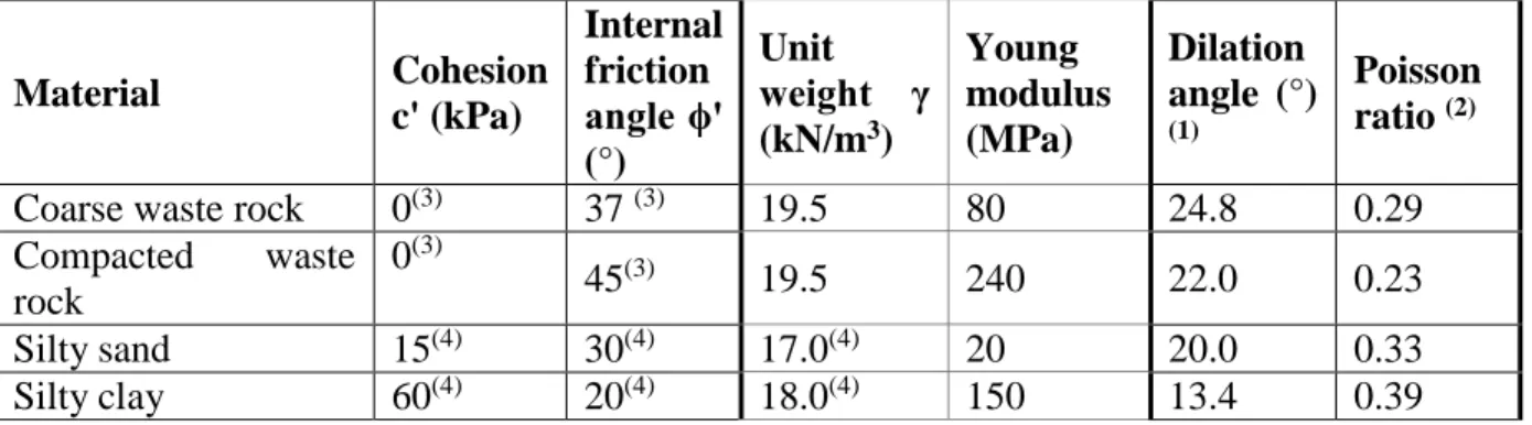
Table 4-3: Geotechnical parameters of the different materials used for the analyses (basic values) ... 84 Table 4-4: Geometric configuration of the waste rock piles used for the stability analysis ... 86 Table 4-5: Additional details on Groups 1 to 9 (Cases S1 to S51) ... 89 Table 4-6: FS and position of center of rotation for shallower slip surfaces (see Figure 4-10)

obtained with different methods (Case S1 with capp = 1 kPa) ... 101

Table 4-7: FS and details of center of rotation for different method (Case S11), capp =1 kPa ... 108

Table 4-8: FS and centers of rotation for critical local slip surfaces with different methods (Case S21, capp =1 kPa) ... 112

Table 4-9: Effect of pile height H (m) and value of cohesion C = capp (kPa) on FS and the position

of the critical slip surface with minimum depth of 1 m (for the deepest slice) ... 133 Table 5-1: Different rainfalls imposed in this study (duration and intensity) ... 147 Table 5-2: Minimum local factor of safety during rainfall (2.7×10-4 m/d, R 2-2) for different

cases ... 174 Table 5-3: Minimum global factor of safety during rainfall (2.7×10-4 m/d, R 2-2) for different

cases ... 174 Table 5-4: Minimum local factor of safety during rainfall R 5-2 (0.001 m/d) for different cases ... 176 Table 5-5: Minimum global factor of safety during rainfall R (0.001 m/d) for different cases ... 176 Table 5-6: Initial and the minimum factor of safety FS for a local slip surface for different cases

with the imposed rainfall R 2-1 ... 179 Table 5-7: Initial and the minimum factor of safety for a global slip surface for different cases

under rainfall R 2-1 ... 179 Table 5-8: Initial and the maximum factor of safety for a global slip surface for different cases

under rainfall R 2-1 ... 181 Table 5-9: Initial and minimum factor of safety for local and global slip surface, Case S11 with

(16)

Table 5-10: Initial and the minimum factor of safety for local slip surface during rainfall R 1 .. 194 Table 5-11: Initial and the minimum factor of safety for a global slip surface under rainfall R 1 ... 196 Table 5-12: Initial and minimum factor of safety for the local slip surface for different rainfalls ... 199 Table 5-13: Initial and minimum factor of safety for a local slip surface, under different rainfalls

R 3-1, R 3-2 and R 3-3 ... 210 Table 5-14: Initial and minimum factor of safety for a global slip surface, under different rainfall

R 3-1, R 3-2, and R 3-3 ... 210 Table 5-15: Reduction (%) of local and global factor of safety comparing different depths of slice

surface, Case S21, rainfall R 1 ... 214 Table 6-1: Mean and standard deviation values for φꞌ and γ and c ... 225 Table 6-2: Results obtained with Monte-Carlo slope stability analyses, using a COV 10% for ϕꞌ,

(17)

LIST OF FIGURES

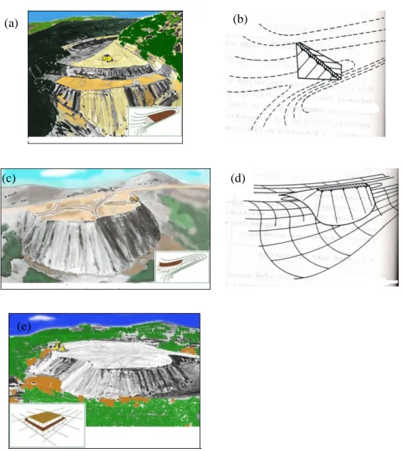
Figure 2-1: Different construction types, a) Valley fill pile; b) Cross-valley fill; c) Sidehill fill pile; d) Ridge crest pile; e) Heaped pile (a, c and e adapted from McCarter (1990), taken

from Aubertin et al., (2002a), b and d Wahler (1979) ... 7

Figure 2-2: Construction of waste rock piles using end dumping; during (a) and after (b) McLemore et al. (2009); during (c), after (d) Martin (2004) ... 9

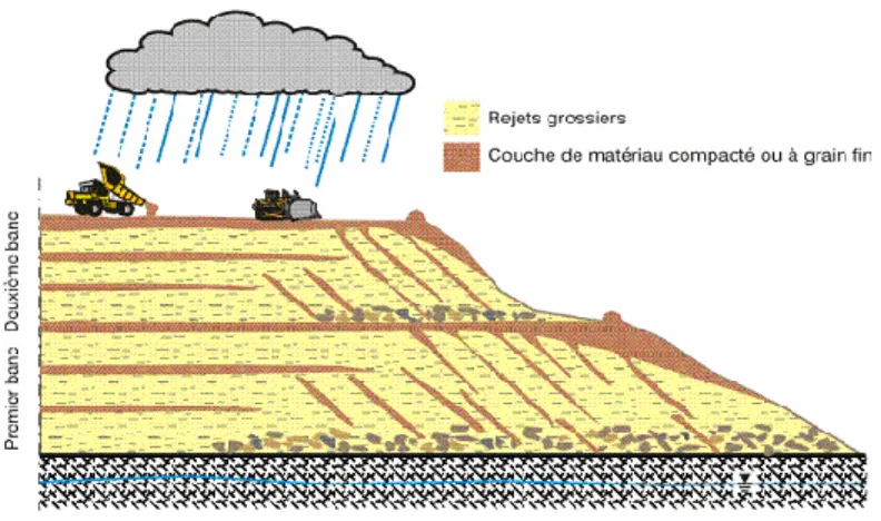
Figure 2-3: Sectional view of a waste rock pile with segregation along the slope (Aubertin et al., 2005) ... 11

Figure 2-4: Grain size distribution curves from literature- see details in Table 2-1 ... 12

Figure 2-5: Correlations between the internal friction angle and density for different soil types, adapted from Navfac (1982); Holtz et al. (2010) ... 15

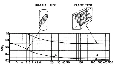
Figure 2-6: Estimation of equivalent strength (S) of rockfill based on D50 value (cited by Barton, 2008) ... 16

Figure 2-7: Empirical method to estimate the equivalent roughness R of rockfill as a function of porosity and particle origin, roundness and smoothness (adapted from Barton and Kjaernsli, 1981) ... 17

Figure 2-8: Effect of particle shape on critical state friction angle for sand, adapted from Cho et al. (2006) ... 18

Figure 2-9: Variation of peak internal friction angle with effective normal stress for direct shear tests on standard Ottawa sand, adapted from Das (1983) ... 19

Figure 2-10: Peak shear strength data for rockfills from Leps (1970) adopted from Barton (2008) ... 20

Figure 2-11: The unsaturated zone and the natural hydrologic cycle (Lu and Likos, 2004) ... 21

Figure 2-12: Typical soil profile showing positive and negative pore pressures ... 22

Figure 2-13: Schematic representation of a water retention curve for soil (Fala 2008) ... 23

Figure 2-14: Schematic presentation of water retention curve for two types of soil, modified by Aubertin et al. (2002a) ... 26

(18)

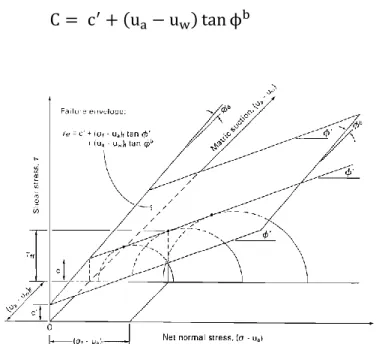
Figure 2-15: Schematic presentation of hydraulic conductivity curve for two types of soil, modified by Aubertin et al. (2002a) ... 29 Figure 2-16: Extended Mohr-Coulomb failure envelope for soils with matric suction ... 35 Figure 2-17: Deterministic and statistical description of soil property (taken from Griffiths, 2007) ... 49 Figure 2-18: Comparison of two probabilistic analysis of a pile foundation (adopted from El-Ramly (2001) modified from Lacasse (1996 ) ... 56 Figure 2-19: Nominal probability of failure for normally distributed FS as function of reliability

index, adapted from Christian et al. (1994) ... 57 Figure 3-1: Elastic-perfectly plastic constitutive relationship (GeoSlope International Ltd, 2008) ... 61 Figure 3-2: Movement areas of points in the optimization procedure, taken from Krahn (2007c)69 Figure 3-3: Typical mesh configuration for a typical model simulation (in SEEP/W and

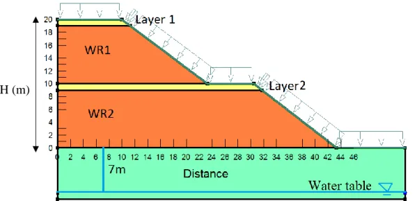
SIGMA/W), Case S21 ... 71 Figure 3-4: Geometry and regions for the simulated waste rock pile (Case S21) under transient

conditions (rainfall of 5.78×10-7 m/s, duration of 24 hrs; capp=1 kPa) to evaluate numerical

convergence issues. ... 74 Figure 3-5: Points representing the nodes in Layer 1 for convergence issues ... 75 Figure 3-6: Volumetric water content versus suction for nodes in Layer 1 after rainfall 5.78×10-7

m/s with 24 hr duration compared to the imposed water retention curve ... 75 Figure 3-7: Volumetric water content versus suction for nodes in Layer 2 after rainfall 5.78e×10-7

m/s with 24hr duration compared to the water retention curve of the compacted waste rock ... 76 Figure 3-8: Points representing the nodes in WR1 to be checked for convergence issues ... 76 Figure 3-9: Volumetric water content versus suction for nodes in WR1 (a) and WR2 (b) after a

rainfall of 5.78x10-7 m/s with 24 hr duration compare to WRC of the loose and compacted waste rocks ... 77

(19)

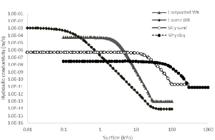
Figure 4-1: Water retention curves for the four materials (compacted and coarse WR, silty sand and silty clay) used in the analyses ... 82 Figure 4-2: Hydraulic conductivity functions used in the analyses for the four materials

(compacted and coarse WR, silty sand, and silty clay) ... 82 Figure 4-3: Dimensions of the foundation used for the simulations performed with GeoStudio

(SEEP/W, SIGMA/W, and SLOPE/W; see text for details) ... 90 Figure 4-4: Effect of the model foundation size (length LF and height HF see Figure 4-3) on the

factor of safety of waste rock pile for Cases S1 and S11 (with capp = 0); Foundation material:

waste rock or silty sand; simulation with SIGMA/W and SLOPE/W ... 91 Figure 4-5: Displacements boundary conditions for simulations with SIGMA/W (Cases S1 left

and S11 right) ... 91 Figure 4-6: Values of capp versus suction, based on Equation 4-1, implemented in SIGMA a)

coarse waste rock (with ϕꞌ = 37°); b) compacted, fine waste rock (ϕꞌ = 45°), based ... 93 Figure 4-7: PWP distribution for Case S1 (capp =1 kPa) along lines A and B obtained with

SIGMA/W ... 95 Figure 4-8: Total vertical stress σy contours (kPa) computed with SIGMA/W (Case S1, with capp

=1 kPa) ... 95 Figure 4-9: Vertical effective stress σ'y contours (kPa) computed with SIGMA/W (Case S1, with

capp =1 kPa) ... 96

Figure 4-10: Relatively shallow critical slip surfaces, center of rotation, and FS obtained with SLOPE/W using different methods (Case S1, capp=1 kPa; a) Morgenstern-Price (MP)

method; b) Optimized FS-stress based method; c) FE stress-based method; d) Simplified Bishop method ... 97 Figure 4-11: Relatively deep critical slip surfaces, center of rotation, and FS obtained with

SLOPE/W using different methods (Case S1 capp=1 kPa; a) Morgenstern-Price (MP)

method; b) Optimized FS-stress based method; c) FE stress-based method; d) Simplified Bishop method ... 98

(20)

Figure 4-12: Distribution of the shear stress mobilized (a), shear strength (b) and effective normal stresses (c) along relatively shallow critical slip surface (see Figure 4-10) for different analysis methods (Case S1 capp=1 kPa), obtained with SLOPE/W ... 100

Figure 4-13: Local factor of safety per slice for the different analysis methods (FE stress-based method, Optimized FE stress-based method, simplified Bishop, MP), Case S1, capp= 1 kPa

... 101 Figure 4-14: PWP distribution for Case S11 (capp =1 kPa) along lines A, B, C, and D obtained

with SIGMA/W ... 102 Figure 4-15: Total vertical stress σy contours (kPa) computed with SIGMA/W (S11) for capp =1

kPa ... 103 Figure 4-16: Vertical effective stress σ'y contours (kPa) computed with SIGMA/W (Case S11,

with capp =1 kPa). ... 103

Figure 4-17: Relatively shallow critical slip surfaces, center of rotation and FS obtained with SLOPE/W using different methods (Case S11, capp=1 kPa); a) Morgenstern-Price (MP)

method; b) Optimized FS stress-based method; c) FE stress-based method; d) Simplified Bishop method ... 104 Figure 4-18: Relatively deeper critical slip surfaces (entering the crest and exiting the toe), related

center of rotation obtained with SLOPE/W using different methods (Case S11, capp=1 kPa);

a) Morgenstern-Price method (MP); b) Optimized FS based method; c) FE

stress-based method; d) Simplified Bishop method ... 105

Figure 4-19: Distributions of the a) shear stress mobilized; b) shear strength; c) effective normal stresses; along critical slip surface for different analysis methods obtained with SLOPE/W (see also Figure 4-18) ... 107 Figure 4-20: Local factor of safety per slice for different methods (FE stress-based, Optimized

FE stress-based, simplified Bishop, MP), Case S11, capp=1 kPa ... 109

Figure 4-21: PWP distribution for Case S21, capp =1 kPa, along lines A, B, C, and D obtained

(21)

Figure 4-22: Total vertical stress σy contours (kPa) computed with SIGMA/W (S21, for capp =1

kPa) ... 110 Figure 4-23: Vertical effective stress σ'y contours (kPa) computed with SIGMA/W (Case S21,

capp =1 kPa) ... 110

Figure 4-24: Distributions of the a) shear stress mobilized; b) shear strength; c) effective normal stresses, along local critical slip surface (Case S21, capp =1 kPa) for different analysis

methods obtained with SLOPE/W ... 111 Figure 4-25: Local factor of safety per slice obtained with different methods (Case S21, capp =1

kPa) ... 112 Figure 4-26: Slope geometry for Cousinsꞌ chart, adapted from Coduto (1999) ... 113 Figure 4-27: One of Cousinsꞌs (1978) charts for failure analysis through the toe of slopes with

zero pore water pressure (adapted from American Society of Civil Engineers) ... 114 Figure 4-28: Factor of safety of a homogenous waste rock pile (Case S1, Table 4-4), for different

ϕ' (= 30 to 50°) and C ( = capp = 0, 10, 25 and 50 kPa); obtained with SIGMA/W and

SLOPE/W (FE stress-based method) compared with results from the Cousinsꞌ (1978) charts (for c > 0) and from the basic slope stability relationship (FS = tanϕ'/tanα, for c = 0) ... 116 Figure 4-29: Relationship between the factor of safety FS and the dimensionless ratio capp/γHt, for

waste rock piles with ϕꞌ = 30°, 37° and 45° and capp= 1, 5, 10 and 25 kPa; a) Case S1; b)

Case S11 ; c) Case S21 ; d) Case S31; e) Case S35 (see Tables 4-4 and 4-5 for details) .... 117 Figure 4-30: Distribution a) shear strength; b) mobilized stress state; c) normal stress; d) local FS;

along the critical slip surface, Case S1, capp (= 1, 5, 10 and 25 kPa); results obtained with

Optimized FE stress-based method ... 118

Figure 4-31: Relationship between the factor of safety FS and the dimensionless ratio capp/γHt, for

waste rock piles with ϕꞌ = 30°, 37° and 45°; capp= 1, 5, 10 and 25 kPa; a) Case S2; b) Case

S12; c) Case S22; d) Case S32; e) Case S36; f) typical global slip surface obtained with

Optimized FE stress-based method ... 120

Figure 4-32: Relationship between the factor of safety FS and pile height Ht; a) Group 1(Cases S1

(22)

(Cases S21 to S24, Ht = 20 m to 120 m); d) Group 6 (Cases S31 to S34, Ht = 20 m to 120

m); e) Group 3 (Cases S15 to S17, Ht = 40 m to 120 m); f) Group 5 (Cases S25 to S27, Ht =

40 m to 120 m); ϕꞌ = 37° and capp = 1, 5, 10 and 25 kPa ... 122

Figure 4-33: Relationship between FS and the global slope angle ɑ (= 26, 30 and 37°) obtained with Optimized FE stress-based method; capp = 1, 5, 10 and 25 kPa, ( = 37°), a) H= 20 m,

(Cases S1, S11, S18); b) H=80 m, (Cases S3, S16, S19,); c) H=40 m, (Cases S2, S5, S6); capp = 1, 5, 10 and 25 kPa; d) Typical two bench waste rock pile with local (β) and global (α)

slope angle. ... 123 Figure 4-34: Relationship between the factor of safety FS and the number of benches, (α = 26°, β

= 37°) ; Group 1 (Cases S2 to S4), Group 2 (Cases S12 to S14) and Group 3 (Cases S15 to S17); a) capp = 5 kPa; b) capp= 10 kPa; c) capp = 25 kPa ... 125

Figure 4-35: Relationship between FS and addition of compacted layers; Groups 2 (Cases S11 to S14, Ht = 20 m to 120 m) and Group 4 (Cases S21 to S24, Ht = 20 m to 120 m), ϕꞌ = 37°; a)

local critical surface, capp = 0, b) global critical surface, capp= 0; c) local critical surface

capp=1 kPa; d) global critical surface, capp= 1 kPa ... 126

Figure 4-36: Relationship between FS, height and compacted layers obtained with FE

stress-based method; Group 3 (Cases S15 to S17, Ht = 40 m to 120 m) and Group 5 (Cases S25 to

S27, Ht = 40 m to 120 m), ϕꞌ = 37° (waste rock) and 45° (compacted waste rock); a) local

slip surface, capp= 0, b) global slip surface capp= 0, c) local slip surface, capp= 1 kPa; d) global

slip surface, capp= 1 kPa ... 127

Figure 4-37: Relationship between FS, height and inclined compacted layers obtained with FE

stress-based method; Group 4 (Cases S11 to S14, Ht = 20 m to 120 m), Group 6 (Cases S31

to S34, Ht = 20 m to 120 m) and Group 7 (Cases S35 to S38, Ht = 20 m to 120 m), ϕꞌ = 37°

(waste rock) and 45° (compacted waste rock); a) local critical surface capp=0, b) global

critical surface capp=0; c) local critical surface capp=1 kPa; d) global critical surface capp= 1

kPa ... 128 Figure 4-38: Effect of addition of alternate layers parallel to external slope on FS for piles from

Group 4 (Cases S21 to S24, Ht = 20 m to 120 m) and Group 8 (Cases S41 to S44, Ht = 20 m

(23)

with capp= 0 b) global FS with capp= 0; c) local FS with capp= 1 and d) global FS with capp= 1;

e) Typical local slip surface for Group 8 (with slices); f) Typical global slip surface for Group 9 (with slices). ... 130 Figure 4-39: Relationship between FS and the properties of the foundation material (c and ϕꞌ,

waste rock, silty sand and silty clay), Groups 1, 3, 4 and 5 (Cases S1, S21, S31, and S35); a) Group 1(capp = 1 kPa); b) Group 3 (capp = 0); c) Group 4 (capp = 0); d) Group 5 (capp = 0) .. 132

Figure 4-40: a) distribution of normal stresses (obtained with SIGMA/W), Case S11 (with capp =

0 kPa), b) distribution of variable ϕꞌ, c) factor of safety (1.316) and center of rotation for the local slip surface; d) factor of safety (1.522) and center of rotation for the global slip surface ... 136 Figure 4-41: Distribution a) shear strength, b) shear mobilized, c) normal stress, d) local FS,

along the surface for waste rock pile with capp =0, Case S11, with variable ϕꞌ (37.2° and

33.7°) and constant ϕꞌ = 37°, for global slip surface obtained with SLOPE/W ... 137 Figure 4-42: a) distribution of normal stress (obtained with SIGMA/W), Case S12 (with capp = 0

kPa; b) distribution of variable ϕꞌ; c) factor of safety (1.156) and center of rotation for the local slip surface; d) factor of safety (1.407) and center of rotation for the global slip surface ... 138 Figure 4-43: Distribution a) shear strength; b) shear mobilized; c) normal stress; d) local FS,

along the global slip surface, capp = 0, Case S12, variable ϕꞌ (37.2° to 32°) and constant ϕꞌ =

37°, obtained with SLOPE/W ... 139 Figure 4-44: Variation of factor of safety due to variation of ϕꞌ, a) Group 1 (Cases S1 to S4, Ht =

20 m to 120 m); b) Group 2 (Cases S11 to S14, Ht = 20 m to 120 m), local slip surface; c)

Group 2, global slip surface; d) Group 3 (Cases S15 to S17, Ht = 40 m to 120 m), local slip

surface; e) Group 3, global slip surface, capp =0, single ϕꞌ = 37° and variable ϕꞌ between

37.2° to 32°) ... 140 Figure 5-1: Steps used to conduct the simulation process for slope analysis of the waste rock piles

(24)

Figure 5-2: Model used with SIGMA/W, water table position (-7 m from the base) (step 1) for different cases of waste rock piles (Case S1 on the right, S21 on the left; details in Tables 4-4 and 4-4-5), ... 14-44-4 Figure 5-3: Pore water pressure distribution in the silty sand foundation (Case S1) before the

rainfall; isocontours on the left and distribution along Line A on the right ... 145 Figure 5-4: Infiltration boundary condition with a constant rate (m/s) applied on the waste rock

pile and foundation (presented with SEEP/W) ... 146 Figure 5-5: Typical slip surfaces exiting at the toe for Case S11 (see Table 4-4) with SLOPE/W;

a) local slip surface (one bench, 3 m deep ); b) global slip surface (two benches, 6 m deep ) ... 148 Figure 5-6: Evolution of the pore water pressures (kPa) with the development of a wetting front,

Case S11 under a constant rainfall 3.16×10-9 m/s (2.7×10-4 m/d, R2-2, Table 5-1); a) before rainfall; b) after 90 days; c) after 180 days; d) after 270 days; e) after 365 days ... 150 Figure 5-7: Evolution of the pore water pressures (kPa) under rainfall 3.16×10-9 m/s (2.7×10-4 m/d , R 2-2), Case S11, after 90, 180, 270 and 365 days along; a) line A; b) line B; c) line C; d) line D; e) location of lines A, B, C, and D ... 152 Figure 5-8: Evaluation of the volumetric water content distribution under rainfall 3.16×10-9_m/s

(2.7×10-4_{m/d, R 2-2), Case S11 with initial VWC ≈ 0.05; a) after 90 days; b) after 180 days;}

c) after 270 days; d) after 365 days ... 153 Figure 5-9: Evolution of the volumetric water content distribution under rainfall 3.16×10-9_m/s

(2.7×10-4 m/d, R 2-2), Case S11, after 90, 180, 270 and 365 days along; a) line A; b) line B; c) line C; d) line D ... 154 Figure 5-10: Evaluation of pore water pressure (kPa) with the development of a wetting front,

Case S21 under rainfall 3.16×10-9 m/s (2.7×10-4 m/d, R2-2); a) before rainfall; b) after 90 days; c) after 180 days; d) after 270 days; e) after 365 days ... 155 Figure 5-11: Evolution of the pore water pressure under rainfall 3.16×10-9 m/s (2.7×10-4 m/d, R2-2), Case S21, after 90, 180, 270 and 365 days along; a) line A; b) line B; c) line C; d) line D; e) compacted layer along line B ... 156

(25)

Figure 5-12: Evolution of the volumetric water content distribution under rainfall 3.16×10-9_m/s

(2.7×10-4_{m/d, R2-2), for Case S21; a) after 90 days; b) after 180 days; c) after 270 days; d)}

after 365 days ... 157 Figure 5-13: Evolution of the pore water pressure under rainfall 3.16×10-9 m/s (2.7×10-4 m/d, R2-2), for Cases S11 and S21, after 365 days along; a) line A; b) line B; c) line C ... 158 Figure 5-14: Evolution of pore water pressure (kPa) with the development of a wetting front,

Case S35 under rainfall 3.16×10-9 m/s (2.7×10-4 m/d, R 2-2); a) before rainfall; b) after 90 days; c) after 180 days; d) after 270 days; e) after 365 days ... 159 Figure 5-15: Evolution of the pore water pressure under rainfall 3.16×10-9 m/s (2.7×10-4 m/d, R

2-2), Case S35, after 90, 180, 270 and 365 days along; a) line A; b) line B; c) line C; d) line D; e) compacted layer along line D ... 160 Figure 5-16: Evolution of volumetric water content distribution under rainfall 3.16×10-9 m/s

(2.7×10-4 m/d, R 2-2), for Case S35; a) after 90 days; b) after 180 days; c) after 270 days; d) after 365 days ... 161 Figure 5-17: Evolution of the pore water pressure under rainfall 3.16×10-9 m/s (2.7×10-4 m/d, R

2-2, Table 5-1), for Cases S21 and S35, after 365 days along; a) line A; b) line B ... 162 Figure 5-18: Evolution of pore water pressure (kPa) with the development of a wetting front,

Case S41, under rainfall 3.16×10-9_{m/s (2.7×10}-4_{m/d, R 2-2); a) before rainfall; b) after 90}

days; c) after 180 days; d) after 270 days; e) after 365 days ... 163 Figure 5-19: Evolution of the pore water pressure under rainfall 3.16×10-9_{m/s (2.7×10}-4_{m/d, R}

2-2), Case S41, after 90, 180, 270 and 365 days along; a) line A; b) line B; c) line C; d) line D ... 164 Figure 5-20: Evolution of volumetric water content distribution under rainfall 3.16×10-9 m/s

(2.7×10-4 m/d, during 365 days), Case S35; a) after 90 days; b) after 180 days; c) after 270 days; d) after 365 days ... 165 Figure 5-21: Evolution of pore water pressure (kPa) with the development of a wetting front,

Case S51 under rainfall 3.16×10-9 m/s (2.7×10-4 m/d, R 2-2); a) before rainfall; b) after 90 days; c) after 180 days; d) after 270 days; e) after 365 days ... 166

(26)

Figure 5-22: Evolution of the pore water pressure under rainfall 3.16×10-9_{m/s (2.7×10}-4_{m/d, R}

2-2), Case S51, after 90, 180, 270 and 365 days along; a) line A; b) line B; c) line C; d) line D; e) Layer line B ... 167 Figure 5-23: Evolution of volumetric water content distribution under rainfall 3.16×10-9 m/s

(2.7×10-4 m/d, R 2-2), Case S51; a) after 90 days; b) after 180 days; c) after 270 days; d) after 365 days ... 168 Figure 5-24: Evolution of the pore water pressure under rainfall 3.16×10-9 m/s (2.7×10-4 m/d, R

2-2), after 365 days along Line B; a) Cases S41 and S51; b) Cases S21 and S41; c) Cases S35 and S51 ... 169 Figure 5-25: Evaluation of local minimum factor of safety under rainfall R 2-2; a) Case S11; b)

Case S21; c) Case S35; d) Case S41; e) Case S51; f) Cases S11, S21, S35, S41, and S51; g) typical local slip surface Case S11; h) typical local slip surface Case S35 ... 171 Figure 5-26: Variation of minimum factor of safety of Global slip surface under rainfall R 2-2; a)

Case S11; b) Case S21; c) Case S35; d) Case S41; e) Case S51; f) Cases S11, S21, S35, S41, and S51; g) typical global slip surface for Case S11 ... 173 Figure 5-27: Variation of minimum factor of safety (local and global slip surface) obtained for

different cases (S11, S21, S35, S41, S51) during rainfall R 5-2; a) local FS; b) global FS; c) typical local slip surface for Case S11; d) typical global slip surface for Case S11 ... 175 Figure 5-28: Variation of factor of safety for local and global slip surfaces during and after a 24-hour rainfall 1.157×10-6_{m/s (0.1 m/d, R 2); Cases S21, S35, S41, and S51 (see Tables 4-4}

and 4-5); a) local slip surface, initial suction equal to WEV; b) global slip surface, initial suction equal to WEV; c) local slip surface, initial suction of 2 WEV; d) global slip surface, initial suction of 2 WEV; e) local slip surface, initial suction of 3 WEV; f) global slip surface, initial suction of 3 WEV ... 178 Figure 5-29: Variation of the factor of safety for local slip surfaces during rainfall R 2-1, with 3

different initial suction (WEV or residual, 2WEV or 2 residual, and 3WEV or 3 residual); a) Case S21; b) Case S35; c) Case S41; d) Case S51. ... 180

(27)

Figure 5-30: Variation of factor of safety for Global slip surface with respect to time during and after rainfall R 2-1, with 3 different initial suction WEV or residual, 2WEV or 2 residual, and 3WEV or 3 residual); a) Case S21; b) Case S35; c) Case S41; d) Case S51 ... 182 Figure 5-31: Variation of different parameters along the local slip surface, with respect to time (6,

12, 18, 24 hours) under a rainfall of 1.157×10-6 m/s (0.1 m/d, R 2-1), Case S21, initial suction 2WEV; a) negative pore water pressure; b) strength due to apparent cohesion; c) shear mobilized; d) shear strength; e) factor of safety ... 184 Figure 5-32: Evaluation of factor of safety during and after rainfall R 2-1, for three different

initial apparent cohesion (capp = 1, 5 and 10 kPa), Case S11; a) local slip surfaces; b) global

slip surfaces ... 185 Figure 5-33: Variation of the PWP along local slip surface under rainfall R 2-1, Case S11; a) capp

= 1 kPa; b) capp = 5 kPa; c) capp = 10 kPa ... 187

Figure 5-34: Variation of the PWP along global slip surface under rainfall R 2-1, Case S11; a) capp = 1 kPa; b) capp = 5 kPa; c) capp = 10 kPa ... 188

Figure 5-35: Variation of the PWP with the wetting front in Case S21 under rainfall 1.736×10-6 m/s (0.15 m/d, R 3-3, Table 5-1) at different time steps (t=0, 6, 12, 18 and 24 hrs); a) line A; b) line B; c) line C; d) line D; e) pile with location of lines A, B, C and D; f) typical local slip surface for Case S21 ... 190 Figure 5-36: Evolution of the volumetric water content distribution, Case S21, under rainfall

1.736×10-6_{m/s (0.15 m/d, R 3-3) at different time steps; a) line A; b) line B; c) line C; d)}

line D (see other details in Figure 5-35 and Table 5-1) ... 191 Figure 5-37: Variation of the local factor of safety over time during and after rainfall 5.78 ×10-7 m/s (0.05 m/d, R 1); a) Case S11; b) Case S21; c) Case S35; d) Case S41; e) Case S51; f) Cases S11, S21, S35, S41 and S51 ... 193 Figure 5-38: Variation of the global factor of safety over time during and after rainfall 5.78 ×10-7 m/s (0.05 m/d, R 1) for a global slip surface; a) Case S11; b) Case S21; c) Case S35; d) Case S41; e) Case S51; f) Cases S11, S21, S35, S41 and S51 ... 195 Figure 5-39 (continued): Variation of factor of safety with respect to time during and after

(28)

rainfall R 2, global slip surface; c) rainfall R 3-3, local slip surface; d) rainfall R 3-3, global slip surface; e) rainfall R 4, local slip surface; f) rainfall R 4, global slip surface; g) rainfall R 5, local slip surface; h) rainfall R 5, global slip surface ... 198 Figure 5-40: Pore water pressures distribution along a local slip surface (at midpoint of each slice

at the base) under rainfall 1.73×10-6 m/s (R 3-3); a) Case S11; b) Case S21; c) Case S35; d) Case S41; e) Case S51; f) typical local slip surface for Case S11 ... 200 Figure 5-41: Variation of strength due to the suction (kPa) along a local slip surface at the

midpoint of each slice, under rainfall 1.73×10-6 m/s (0.15 m/d, R 3-3), for different time steps; a) Case S11; b) Case S21; c) Case S35; d) Case S41; e) Case S51; f) variation of FS over time for all cases ... 202 Figure 5-42: Variation of the factor of safety during and after different rainfalls (R 1, R 2-1, R 3-3, R 4 and R 5-1), for local slip surfaces; a) Case S11; b) Case S21; c) Case S35; d) Case S41; e) Case S51 ... 204 Figure 5-43: Variation of factor of safety during and after different rainfalls (R 1, R 2-1, R 3-3, R

4 and R 5-1), for a global slip surface; a) Case S11; b) Case S21; c) Case S35; d) Case S41; e) Case S51 ... 206 Figure 5-44: Variation of factor of safety for local slip surface under rainfall R 3-1, R 3-2, and R

3-3; a) Case S21; b) Case S35; c) Case S41; d) Case S51 ... 208 Figure 5-45: Variation of factor of safety for Global slip surface under rainfall R 1 (6 hrs), R 3-2 (13-2 hrs) and R 3-3 (3-24 hrs); a) Case S3-21; b) Case S35; c) Case S41; d) Case S51 ... 3-209 Figure 5-46: Variation of the factor of safety for local and global slip surfaces under rainfall R 2-1, different groundwater levels (located 2-1, 3 and 7 m below the ground surface); a) local slip surface, Case S11; b) global slip surface, Case S11; c) local slip surface, Case S21; d) global slip surface, Case S21; e) local slip surface, Case S35; f) global slip surface, Case S35 .... 212 Figure 5-47: Variation of factor of safety for local and global slip surface under rainfall R 1 for

Case S21; a) local slip surface with different depth (3, 2, 1, 0.5 and 0.1 m; b) global slip surface with different depth (6, 5, 4, 3, 2 and 1 m) ... 213

(29)

Figure 5-48: Variation of Wetting front (PWP changes, kPa) for Case S21 after 24 hours , under different k anisotropy under rainfall R 2-1 for 24 hours; a) ky/kx = 0.01; b) ky/kx = 0.1; c)

ky/kx = 1; d) ky/kx = 10; ky/kx = 100 ... 215

Figure 5-49: Changes of factor of safety during and after rainfall R 2-1 for local slip surface, different kxy anisotropy 0.01, 0.1, 1, 10 and 100; a) Case S11; b) Case S21; c) Case S35 .. 216

Figure 5-50: Variation of factor of safety during and after rainfall R 2-1 for global slip surface and different kxy anisotropy 0.01, 0.1, 1, 10 and 100; a) Case S11; b) Case S21; c) Case S35

... 217 Figure 5-51: Variation of factor of safety with time during and after rainfall R 2-1 for local and

global slip surface, Case S11, foundation silty sand, silty clay and waste rock, initial suction 6 kPa; a) local slip surface; b) global slip surface ... 218 Figure 5-52: Changes of factor of safety during and after rainfall R 2-1 for Cases S21, S22, S23,

and S24; a) local slip surface; b) global slip surface ... 219 Figure 6-1: Flow chart of the framework used for probabilistic analyses ... 221 Figure 6-2: Various slip surfaces for a two bench pile (Group 2); a) local slip surface involving ≤

50% Ht); b) slip surface involving 60% Ht; c) slip surface involving 70% Ht; d) slip surface

involving 90% Ht; e) global slip surface, 100% Ht through the toe ... 222

Figure 6-3: a) Probability density function for φꞌ (loose and compacted waste rock, COV 10% and 15%); b) Sampling function for φꞌ (loose and compacted waste rock, COV 10% and 15%); c) Probability density function for γ (loose and dense waste rock, COV 10%); d) Sampling function for γ (loose and dense waste rock, COV 10%) ... 224 Figure 6-4: Normal distribution of the factor of safety for COV% = 10 (ϕꞌ, ϕꞌ and γ), Case S11

(see Tables 4-4 and 4-5 ), for sampling distance = 8 m; a) local slip surface (see Figure 6.2 (a)); b) global slip surface (Figure 6.2 (b)) ... 226 Figure 6-5: Normal distribution of FS obtained with Monte-Carlo simulations (SLOPE/W), COV

= 10% on φꞌ, capp = 1 kPa; sampling distances (SD): 1 m, 3 m, 5 m, 8 m, 12 m, 15 m, per

(30)

b) critical global slip surface, Case S11; c) critical local slip surface, Case S21 (two benches with compacted layers); d) critical global slip surface for Case S21 ... 227 Figure 6-6: FS , RI and PoF distribution for different sampling distance (sampling once; 1, 3, 5, 8,

12 and 15m; sampling per slice), COV 10%, obtained with SLOPE/W; a) FS for local slip surface, Case S11; b) FS for global slip surface, Case S11; c) FS for local slip surface, Case S21; d) FS global slip surface Case S21; e) PoF for local slip surfaces, Cases S11 and S21; f) RI for local and global slip surfaces, Cases S11 and S21 ... 229 Figure 6-7: Normal distribution of FS for slip surface involving 60% Ht obtained with

Monte-Carlo method of SLOPE/W for different COV (10%, 15%); a) Case S1; b) Case S2; c) Case S3; d) Case S4 ... 231 Figure 6-8: Effect of COV% (10%, 15%) on FS , RI, PoF and Standard deviation for a slip

surface involving 60% Ht, obtained with Monte-Carlo method (SLOPE/W), Group 1 (Cases

S1, S2, S3, and S4); a) FS ; b) RI; c) PoF (%); d) Standard deviation ... 232 Figure 6-9: Effect of COV% (10%, 15%) on FS , RI, PoF and Standard deviation for a slip

surface involving 60% Ht, obtained with Monte-Carlo (SLOPE/W), Group 2 (Cases S11,

S12, S13, and S14); a) FS ; b) RI; c) PoF (%); d) Standard deviation ... 233 Figure 6-10: Normal distribution of FS based on different iterations numbers, Case S21, slip

surface involving 60%Ht; a) COV 15%; b) COV 10% ... 234

Figure 6-11: Distribution of FS , RI and standard deviation due to different iteration numbers, obtained with Monte-Carlo method (SLOPE/W), slip surface involving 60%Ht, COV 10%

and 15%; a) FS ; b) RI; c) Standard deviation ... 235 Figure 6-12: Distribution functions of FS produced with Monte-Carlo method, COV = 15% for

selected slip surface involves 60% Ht; capp= 5, 10 and 25 kPa, a) Case S1; b) Case S2; c)

Case S15; d) Case S16 (see Tables 4-4 and 4-5 for details) ... 237 Figure 6-13: FS with Monte-Carlo method, COV = 15%, for different capp (= 5, 10 and 25 kPa,

imposed as suction), Group 1, a) slip surface involving 60% Ht; b) slip surface involving

(31)

Figure 6-14: RI distribution for COV 15% (ϕꞌ), different capp (= 5, 10 and 25 kPa), Group 1, a)

slip surface involving 60% Ht; b) slip surface involving 70% Ht; c) slip surface involving

90% Ht ... 239

Figure 6-15: PoF (%) distribution for COV 15%, different capp (= 5, 10 and 25 kPa), Group 1, a)

slip surface involving 60% Ht; b) slip surface involving 70% Ht; c) slip surface involving

90% Ht ... 240

Figure 6-16: FS and RI distribution, COV 15% (ϕꞌ), different capp (= 5, 10 and 25 kPa), for slip

surfaces involving 60% and 90% Ht; a) FS, Group 2 (Cases S11, S12, S13, S14, Ht 20, 40,

80, 120 m); b) RI, Group 2; c) FS, Group 2; d) RI, Group 2; e) FS, Group 3 (Cases S15, S16, S17, Ht 40, 80, 120 m; f) RI, Group 3; g) FS, Group 3; h) RI, Group 3 ... 242

Figure 6-17: Normal distribution of FS for slip surface involving 60% Ht obtained with

Monte-Carlo method (SLOPE/W), COV= 15%, C (=5, 10 and 15 kPa); a) Case S11; b) Case S12; c) Case S13; d) Case S14 ... 244 Figure 6-18: Distribution of FS, RI and PoF obtained with the Monte-Carlo (SLOPE/W), COV =

15% (φꞌ and C), C = 5, 10 and 15 kpa, Group 2 (Cases S11, S12, S13, S14, Ht = 20, 40, 80,

120 m); a) FS ; b) RI; c) PoF ... 245 Figure 6-19: Normal distribution of FS for local slip surface obtained with Monte-Carlo method (

SLOPE/W), COV 15% (ϕꞌ and C), C (=5, 10 and 15 kPa); a) Case S21; b) Case S22; c) Case S23; d) Case S24 ... 246 Figure 6-20: Distribution of FS, RI and PoF obtained with Monte-Carlo (SLOPE/W), COV =

15% (ϕꞌ and C = 5, 10 and 15 kpa), Group 2 (Cases S21, S22, S23, S24); a) FS ; b) RI; c) PoF ... 247 Figure 6-21: Effect of number of benches on FS and RI, COV = 15% (ϕꞌ), sampling distance ½

Ht, capp= 5 kPa, Group 1 (Cases S1, S2, S3, S4, Ht = 20, 40, 80, 120 m), Group 2 (Cases S11,

S12, S13, S14, Ht = 20, 40, 80, 120 m), Group 3 (Cases S15, S16, S17, Ht = 40, 80, 120 m);

a) FS , slip surface 60% Ht, Groups 1 and 2; b) RI, slip surface 60% Ht,Groups 1 and 2; c)

FS , slip surface 70% Ht ,Groups 1 and 2; d) RI, slip surface 70% Ht, Groups 1 and 2; e) FS ,

(32)

Figure 6-22: Effect of horizontal layers on the normal distribution of FS, COV 15% (ϕꞌ), slip surface involving 60% Ht, capp= 1 kPa, Group 2 (Cases S11, S12, S13, S14, Ht = 20 m to 120

m), Group 4 (Cases S21, S22, S23, S24, Ht = 20 m to 120 m); a) Cases S11 vs S21; b) Cases

S12 vs S22; c) Cases S13 vs S23; d) Cases S14 vs S24 ... 250 Figure 6-23: Effect of addition of compacted layers on FS and RI, COV 15% (ϕꞌ), capp= 1 kPa,

slip surface involving 60%, 70% and 90% Ht, capp= 1 kPa, Group 2 (Cases S11, S12, S13,

S14, Ht = 20, 40, 80, 120 m), Group 4 (Cases S21, S22, S23, S24, Ht = 20, 40, 80, 120 m);

a) FS , slip surface 60% Ht; b) RI, slip surface 60% Ht; c) FS , slip surface 70% Ht; d) RI,

slip surface 70% Ht; e) FS , slip surface 90% Ht; f) RI, slip surface 90% Ht ... 252

Figure 6-24: Effect of horizontal compacted layers on normal distribution of FS, COV 15% (ϕꞌ), capp= 1 kPa and 2.5 kPa for loose and compacted waste rock, Group 3 (Cases S15, S16, S17,

Ht = 40, 80, 120 m), Group 5 (Cases S25, S26, S27, Ht = 40, 80, 120 m); a) slip surface

involving 60% Ht, Cases S15 vs. S25; b) slip surface involving 70% Ht, Cases S16 vs. S26;

c) slip surface involving 90% Ht, Cases S17 vs. S27 ... 253

Figure 6-25: Effect of compacted layers on FS and RI, COV 15% (ϕꞌ), sampling distance ½ Ht,

capp= 1 kPa and 2.5 kPa for loose and compacted waste rock, Group 3 (Cases S15, S16, S17,

Ht = 40, 80, 120 m), Group 5 (Cases S25, S26, S27, Ht = 40, 80, 120 m); a) FS, slip surface

involving 60% Ht; b) RI, slip surface involving 60% Ht; c) FS, slip surface involving 70%

Ht; d) RI, slip surface 70% Ht; e) FS, slip surface involving 90% Ht; f) RI, slip surface

involving 90% Ht ... 255

Figure 6-26: Effect of inclined layers on FS and RI, COV 15% (φꞌ), sampling distance ½ Ht, capp=

1 kPa, Group 4 (Cases S21, S22, S23, S24, Ht = 20, 40, 80, 120 m), Group 6 (Cases S35,

S36, S37, S38, Ht = 20, 40, 80, 120 m); a) FS, slip surface involving 60% Ht; b) RI, slip

surfaces involving 60% Ht; c) FS, slip surface involving 70% Ht; d) RI, slip surface

involving 70% Ht; e) FS, slip surface involving 90% Ht; f) RI, slip surface involving 90% Ht

... 257 Figure 6-27: Effect of alternate layers on FS and RI, COV 15% (φꞌ), sampling distance ½ Ht, slip

(33)

S35), Group 8 (Case S41), Group 9 (Case S51); a) FS Cases S21 vs. S41; b) RI Cases S21 vs. S41; c) FS Cases S35 vs. S51; d) RI Cases S35 vs. S51 ... 259 Figure 6-28: Effect of alternate layers on FS and RI, COV 15% (φꞌ), sampling distance ½ Ht, slip

surface involving 60%, 70% and 90% Ht, capp= 1 kPa, Group 4 (Case S22), Group 6 (Case

S36), Group 8 (Case S42), Group 9 (Case S51); a) FS Cases S21 vs. S41; b) RI Cases S21 vs. S41; c) FS Cases S35 vs. S51; d) RI Cases S35 vs. S51 ... 260 Figure 6-29: The effect of horizontal layer thickness on the slope stability obtained with Monte-Carlo method (SLOPE/W), COV 15% (φꞌ), sampling distance ½ Ht, global slip surface,

capp= 1 kPa, Case S22; a) FS normal distribution; b) FS; c) RI; d) PoF ... 262

Figure 6-30: Effect of the groundwater level on the probabilistic analysis of slope stability, COV 15% (φꞌ), sampling distance ½ Ht, global slip surface, capp= 1 kPa, foundation silty sand,

Case S11; a) FS; b) RI; c) PoF and standard deviation ... 263 Figure 6-31: Effect of rainfall infiltration on PoF of local slip surface, COV 15% (φꞌ), Cases S11,

S21, S35; a) Rainfall R 3-1; b) Rainfall R 3-2; c) Rainfall R 3-3 ... 264 Figure A-1: Slope geometry for Cousinsꞌ charts, adapted from Coduto (1999) ... 304 Figure A-2: Factor of safety of a single bench homogenous waste rock pile (H = 20 m, α = 26°),

for different values of ϕ' (= 30 to 45°) and C (= 10, 25 and 50 kPa); results obtained with SLOPE/W (Simplified Bishop Method) and from the Cousinsꞌ (1978) charts ... 305 Figure A-3: Factor of safety of a single bench homogenous waste rock pile (H = 20 m, α = 37°),

for different values of ϕ' (= 30 to 45°) and C (= 10, 25 and 50 kPa); results obtained with SLOPE/W (Simplified Bishop Method) and from the Cousinsꞌ (1978) charts ... 305 Figure A-4: Factor of safety of a single bench homogenous waste rock pile (H = 40 m, α = 30°),

for different values of ϕ' (= 30 to 45°) and C (= 25 and 50 kPa); results obtained with SLOPE/W (Simplified Bishop Method) and from the Cousinsꞌ (1978) charts ... 306 Figure A-5: Factor of safety of a single bench homogenous waste rock pile (H = 40 m, α = 37°),

for different values of ϕ' (= 30 to 45°) and C (= 25 and 50 kPa); results obtained with SLOPE/W (Simplified Bishop Method) and from the Cousinsꞌ (1978) charts ... 306

(34)

Figure A-6: Factor of safety of a single bench homogenous waste rock pile (H = 50 m, β = 37°), for different values of ϕ' (= 30 to 40°) and C (= 50 kPa); results obtained with SLOPE/W (Simplified Bishop Method) and from the Cousinsꞌ (1978) charts ... 307 Figure A-7: Comparison of simulation and test results for Test No.2 ... 331

(35)

LIST OF SYMBOLS AND ABBREVIATIONS

AEV Air Entry Value [ML-1T-2]

{A} Vector of actions at the nodes

a, n, m Fitting parameters (model from Fredlund and Xing, 1999) b ln (106_{) [ML}-1_T-2_{], model from Fredlund et al. (1994)}

c Cohesion [ML-1_T-2_]

c' Effective cohesion [ML-1_T-2_]

capp Apparent cohesion [ML-1T-2]

C Capacity

CG Constant material parameter (KCM method, =0.1)

CU Uniformity coefficient (D60/D10) [-]

COV Coefficient of variation

D Demand

D50 Mean particle diameter [L]

Dr (or Gs) Specific gravity [-]

D5 Sieve size that 5% of the particles (by size) passes it [-]

[D] Drained constitutive matrix

e Void ratio[-]

e Natural logarithmic constant (model from Fredlund and Xing, 1999) E Young’s modulus [FL-2]

F Fitting equations (Table 2-7)

(36)

FEM Finite element method

g Gravitational acceleration [LT-2_]

h Hydraulic head [L]

hc Distance from water table to the point of interest [L]

hco Equivalent capillary rise

H, Ht Total height of waste rock pile [L]

Hf Foundation height [L]

{H} The vector of nodal heads

i Slope angle

ID Relative density [-]

k, kw, k(ψ), k(θ) Hydraulic conductivity [LT-1]

kr Relative hydraulic conductivity [-]

ksat, ks Saturated hydraulic conductivity [LT-1]

kx, ky Hydraulic conductivity in x and y-direction [LT-1]

K0 Coefficient of lateral stress

[kw, sat] Hydraulic conductivity matrix

[K] Matrix of coefficients related to geometry and materials properties [L] Coupling matrix

Lf Foundation length [L]

Lt Layer thickness [L]

[M] Element mass matrix MP Morgenstern-Price method m2w Slope of WRC [-], equation [2-7]

(37)

nv, mv Fitting parameter – Model from van Genuchten (1980) [-]

n Porosity

P Predicting equation (Table 2-7)

PMP Probable maximum precipitation PoF, Pf Probability of failure

PWP Pore water pressure

Q Volume of discharge [L-3]

Q Boundary flux [LT-1]

{Q} Flow quantities at the node

R Particle shape – Roundness [-]

RI Reliability index (or β)

S Equivalent strength related to USC, Figure 2-6 Sc Capillary component of the degree of saturation [-]

Sr Residual degree of saturation [-]

Sr Total shear resistance

Ss Specific surface [L2M-1]

Sm Total mobilized (imposed) shear [ML-1T-2]

t Time [T]

ua Pore air pressure [MT-2L-1]

uw Pore water pressure [MT-2L-1]

UCS Uniaxial compressive strength [MT-2L-1] VWC Volumetric water content

W Total weight of a soil slice WEV Water Entry Value [ML-1T-2]

(38)

WRC Water retention curve {X} Vector of field variables

y Dummy variable of integration representing ln (ψ) (Fredlund 1994)

zw Ground water level [L]

α Fitting parameter - Van Genuchten (1980) equation [M-1LT2] or [L-1] α Global slope angle for waste rock pile

α Angle between the base of the slice and the horizontal β Local slope angle for waste rock pile

β Angle of repose

γsub Submerged soil weight [MT-2L-2]

γtotal Wet unit weight [MT-2L-2]

γw Water unit weight [MT-2L-2]

w Density of water [ML-3]

, FS Standard deviation

σy Total vertical stresses [ML-1T-2]

, σn Normal stress [ML-1T-2]

σ'y Vertical effective stress [ML-1T-2]

ε Normal strain [ML-1_T-2_]

τ, τxy Shear strength [ML-1T-2]

a, aev Air Entry Value [ML-1T-2]

ψd Dilatation angle

𝜓 0 Pressure corresponding to zero water content [ML-1T-2]

 Matric suction [ML-1_T-2_]

(39)

, w Volumetric water content [-]

r Residual volumetric water content [-]

s Saturated volumetric water content [-]

λ Pore size distribution index – Brooks and Corey [-] λcϕ Cousinsꞌs (1978) charts parameter [4-2]

ϕ Friction angle [-]

ϕb

Friction angle with respect to matric suction [-]

ϕ' _{Effective internal friction angle [-]}

ϕb Basic angle of friction [-],Barton (1981), Equation 4-2

ϕc Minimum friction angle for soils [-]

Θ Normalized water content [-]

Θq _{Correction factor for tortuosity (Fredlund et al (1994) Model, equation}

[2-5]

μw Dynamic viscosity [ML-1T-1]

μ, µFS Mean

υ Poisson’s ratio Δ Increment

(40)

LIST OF APPENDICES

Appendix A – Additional results for Chapter 4………307 A-1 Comparison between results obtained with the Simplified Bishop slope stability analysis method and Cousin’s Charts………...307 A-2 Comparing the value of factor of safety and center of rotation between previously presented cases by Fredlund (2000) and numerical simulations (calculations performed with Sigma/W and Slope/W) ………...313 A-3 Additional results related to Section 4-3-2: effect of dilatation angle ………..322 A-4 Additional results related to Section 4-7-10: Effect of alternate layers parallel to the slope ………....323 A-5 Plate loading tests to assess the Young modulus (E) of waste rock………..327 Appendix B – Additional results for Chapter 5………...338

B - 1 Mesh sensitivity analysis ………...338 B – 2 Additional results related to effect of prolonged rainfalls (see section 5-6-6)……..345 B – 3 Additional results presenting evolution of PWP and volumetric water content related to Section 5-7-2 ………..346 B - 4 Additional results related to the effect of increasing rainfall on slope stability (see section 5-7-3) ……….352 B - 5 Additional results related to section 5-7-2-3, variation of negative pore water pressure along global slip surface ………353 B - 6 Additional results to evaluate the effect of AEV and WEV of material WRC in transient analysis ………. ………..354 Appendix C – Additional results for Chapter 6……….363

C-1 Additional results related to section 6-4-1 ……….……363 C-2 Additional results related to section 6-4-2 ………..366

(41)

C-3 Additional results related to section 6-4-3……….368 C-4 Additional results related to section 6-4-4……….372

(42)

CHAPTER 1 INTRODUCTION

Waste rock from hard rock mines is produced by the blasting and extraction process Waste rock, which lacks sufficient value for treatment (Tachie-Menson, 2006), is usually transported by trucks (or conveyors) and disposed of in waste rock piles (sometimes called dumps) for long-term disposal. These are among the largest types (by volume, weight or height) of man-made constructions (Robertson, 1982; Wickland and Wilson, 2005; McLemore et al., 2009). Waste rock piles are typically designed and constructed on the ground surface to prevent the retention of water behind or above the pile surface. As a result, most of the piles are unsaturated (Nelson and McWhorter, 1985).

The behaviour and the stability of waste rock piles have not been studied extensively, in part due to their lack of economic significance in the mining process. The most important aspects considered for their design are the general location (preferably near the mine site), transport, placement (based on available equipment), and other short-term economic factors. A few decades ago (starting mainly in the 1980s), environmental organisations and governmental agencies started demanding improvement in the design of waste rock piles on safety and reclamation (Klohn Leonoff Ltd., 1991; Piteau Associates Engineering, 1991). This thesis pursues this line of work by extending the investigation of the slope stability of piles, taking into account the consequences of internal and external structures, hydro-geotechnical properties and rainfall patterns.

This dissertation addresses the issue of slope stability of waste rock piles having characteristics fairly similar to those constructed at various mine sites. The main objective is to develop and apply a general approach to the assessment of the stability of unsaturated waste rock piles under various conditions. The investigation takes into account several influencing factors including internal features and external geometry of the pile, distribution of pore water pressures before, during and after rainfall, and the spatial variability of important geotechnical properties. The study uses numerical simulations as the main tool in the analytical process.

(43)

i. Assess the basic physical and geotechnical characteristics of waste rock and waste rock piles.

ii. Develop (partly) coupled analytical models to investigate the sensitivity of different parameters, including the pile internal features and external geometry (i.e. height, slope angle, compacted layers, the number of benches, etc.), and material properties (i.e. geotechnical and hydrogeological).

iii. Develop models to simulate pore water distribution and stress-strain behaviour, and then assess slope stability analysis of unsaturated waste rock piles under various rainfalls (i.e. recharge conditions).

iv. Implement stochastic analysis of the main input parameters and apply to pile slope stability.

v. Investigate ways to improve slope stability.

vi. Recommend practical means to improve stability and also topics for future research.

This thesis consists of seven chapters. The organisation and the content of each chapter are summarised as follows:

Chapter 1 (current chapter) provides a short introduction to the project and briefly describes the content of the thesis.

Chapter 2 presents a literature review of relevant knowledge on waste rock piles. The chapter starts by presenting different methods for the construction of waste rock piles. This is followed by a description of the geometric configuration of waste rock piles. Previous investigations indicate that the degree of compaction and material (particles) segregation creates internal features within piles. The literature review also includes a summary of the main properties of waste rock, such as grain size distribution, the angle of repose, and initial friction angle. The unsaturated behaviour of granular materials is also addressed in this chapter, and typical hydraulic properties of waste rock (i.e. volumetric water content, hydraulic conductivity) are presented. The influence of negative pore water pressures on strength (i.e. apparent cohesion) is also reviewed, together with seepage flow in the unsaturated zone. The last sections contain a review of slope stability analysis. It includes different methods of slope stability and recalls

(44)

factors that affect stability. Previous studies have shown that the flow and water distribution within waste rock piles are difficult to measure or predict due to the complex internal structure and material characteristics. This chapter finishes with a review of probabilistic analysis, with a definition of the main input and output parameters related to Monte-Carlo analysis. A single factor of safety may not be enough to discuss the stability of a waste rock pile and other parameters (such as the reliability index RI and the probability of failure PoF) can be used to obtain a more complete assessment, these tools are applied later in the thesis.

Chapter 3 describes the approach used for the modelling and the methodology applied for conducting the stability analyses on waste rock piles under unsaturated conditions. The chapter includes a basic description of the problem and presentation of the calculation tools, including the fundamentals of numerical modelling with the finite element combined with limit equilibrium methods. Also, some of the main challenges related to the stability analyses of waste rock piles under unsaturated conditions are briefly addressed.

Chapter 4 presents preliminary results from slope stability analyses for constant conditions in the piles (mainly for dry cases). The effects of apparent cohesion (produced by the matric suction) on the stability of unsaturated waste rock pile are also investigated. The results serve to illustrate the influence of different factors such as pile geometry, waste rock properties and matric suction on the stability of the waste rock pile. These results are obtained by a coupled approach using SIGMA/W and SLOPE/W.

Chapter 5 presents the calculations results on the effect of relatively short and heavy rainfalls on the stability of unsaturated waste rock piles. The results show that the shear strength produced from matric suction can change over time and location due to the evolution of the water distribution. These results are obtained from an (indirect) coupled approach using SEEP/W, SIGMA/W, and SLOPE/W, starting with the pore water pressures, and the stress distributions, which are then used to assess the factor of safety and the critical slip surfaces. The chapter provides specific details on seepage modelling and slope stability analyses for transient conditions. Different rainfall patterns were applied as boundary conditions to evaluate time-dependent phenomena. The presence of loose and compacted waste rock layers was also taken into account. Chapter 6 presents the results related to uncertainties on the stability (and reliability) of waste rock piles. The results demonstrate the effect of having non-unique values for