Intertemporal utiÏity models for asset pricing:
reference levels and individual heterogeneity
par
Andrei $emenov
Département de sciences économiques Faculté des arts et des sciences
Thèse présentée à la Faculté des études supérieures en vue de l’obtention du grade de Philosophiae Doctor (Ph.D.)
en sciences économiques
Août 2003
dh
de Montréal
Direction des bibliothèques
AVIS
L’auteur a autorisé l’Université de Montréal à reproduire et diffuser, en totalité ou en partie, par quelque moyen que ce soit et sur quelque support que ce soit, et exclusivement à des fins non lucratives d’enseignement et de recherche, des copies de ce mémoire ou de cette thèse.
L’auteur et les coauteurs le cas échéant conservent la propriété du droit d’auteur et des droits moraux qui protègent ce document. Ni la thèse ou le mémoire, ni des extraits substantiels de ce document, ne doivent être imprimés ou autrement reproduits sans l’autorisation de l’auteur.
Afin de se conformer à la Loi canadienne sur la protection des renseignements personnels, quelques formulaires secondaires, coordonnées ou signatures intégrées au texte ont pu être enlevés de ce document. Bien que cela ait pu affecter la pagination, il n’y a aucun contenu manquant.
NOTICE
The author of this thesis or dissertation has granted a nonexclusive license allowing Université de Montréal to reproduce and publish the document, in part or in whole, and in any format, solely for noncommercial educational and research purposes.
The author and co-authors if applicable retain copyright ownership and moral rights in this document. Neither the whole thesis or dissertation, nor substantial extracts from it, may be printed or otherwise reproduced without the author’s permission.
In compliance with the Canadian Privacy Act some supporting forms, contact information or signatures may have been removed from the document. While this may affect the document page count, it does not represent any loss of content from the document.
Cette thèse intitu’ée:
IlltCrtemporaÏ u.tiÏity mocÏeÏs for a&et
pricillg:
reference ÏveÏs aiicï iiicÏividia1 iieterogeneity
présentée par:
Andrei Senïenov
a ete evauée pal- un jury compose des personnes suivantes:
P résident—rapporteur: Eznanue]a Cardia
Directeur de recherche: René Garcia
Codirecteur: Éric Renauft
Membre du jury: Rui Castro Examinateur externe- Univ. McGilI: Kris Jacobs
La thèse propose de nouveaux modèles d’évaluation des actifs financiers fondés sur la con
sommation. Ces modèles, soit avec agent représentatif, soit avec consommateurs hétérogènes, permettent de mieux expliquer les primes de risque et le taux sans risque avec des valeurs
raisonnables des paramètres de préférence. De plus, ces modèles emboÎtent, comme cas
particuliers, les modèles les plus connus dans la littérature, ce qui permet des tests de spécification informatifs.
Le premier article introduit la nouvelle fonction d’utilité avec niveau de référence dans
un cadre par ailleurs standard d’agent représentatif. Le deuxième article suggère que la
séparation de l’aversion pour le risque et la substitution intertemporelle peut être obtenue
pas par le remplacement, comme le fait l’utilité récursive, de la consommation future par un équivalent certain de l’utilité future, mais par un niveau de référence exogène qui, d’une
manière récursive, évalue la consommation future attendue. Dans le troisième article, un
modèle avec agents hétérogènes permet de souligner l’importance de l’asymétrie de la dis
tribution en coupe transversale des consommations individuellesdans la caractérisation des
primes de risque. Le quatrième article évalue l’importance de l’hétérogénéité lorsque les
agents ont une utilité avec niveau de référence et teste la fonction d’utilité isoélastique dans
une économie avec agents hétérogènes.
Dans “A Consumption CAPM with a Reference Level”, article conjoint avec René Garcia
et Eric Renault, nous étudions un modèle d’utilité espérée dans lequel un agent dérive son
utilité à la fois de l’excès relatif de sa consommation par rapport à un niveau de référence
et de la valeur absolue de ce niveau de référence. Un des avantages de notre spécification est sa flexibilité. Nous montrons qu’elle peut reproduire la plupart des facteurs d’escompte
stochastiques qui ont été proposés dans la littérature empirique sur l’évaluation des actifs
financiers. Les tests empiriques du modèle avec la consommation agrégée conduisent à
estimer des valeurs économiquement plausibles des paramètres de préférence, contrairement aux deux cas particuliers de la fonction de formation d’habitude et d’utilité non-espérée d’Epstein-Zin. Par ailleurs, nous confirmons l’importance d’inclure le niveau de référence absolu dans la fonction d’utilité.
Level”, article également conjoint avec René Garcia et Eric Renault, nous montrons que si le taux de croissance du niveau de référence dépend du rendement du portefeuille de marché, les conditions de premier ordre pour la fonction d’utilité avec niveau de référence sont équivalentes sur le plan observationnel à ceux qui résultent de la fonction d’utilité récursive d’Epstein-Zin mais conduisent à une interprétation alternative des paramètres de préférence.
Dans “Asset Pricing Puzzles, Higli-Order Consumption Moments, and Heterogeneous Consumers”, nous utilisons une expansion de Taylor de l’utilité marginale pour exprimer l’espérance conditionnelle du rendement de l’actif financier en fonction des moments croisés du rendement avec des moments de la distribution des consommations individuelles. Cette relation permet d’établir si chaque moment augmente ou diminue la prime de risque, sans spécifier une fonction d’utilité particulière. Avec la fonction isoélastique habituelle, nous montrons par callbration et estimation que l’asymétrie de la distribution en coupe transver sale des consommations individuelles joue un rôle essentiel dans l’explication de la prime de risque. Nous obtenons également des valeurs économiquement plausibles des paramètres de préférence.
L’objectif de l’article “An Empirical Assessment of a Consumption CAPM with a Ref erence Level under Incomplete Consumption Insurance” est de tester empiriquement la fonction d’utilité espérée avec niveau de référence proposée dans le premier article sous l’hypothèse d’assurance de consommation incomplète et de participation limitée. Pour ce faire, nous utilisons le modèle d’évaluation des actifs financiers dérivé dans le deuxième article. Nous choisissons assez naturellement comme niveau de référence la consommation agrégée par tête. Lorsque l’asymétrie de la distribution des consommations individuelles et la participation limitée sont prises en compte, on obtient des valeurs économiquement plausibles de tous les paramètres d’intérêt. La fonction d’utilité isoélastique standard et la spécification usuelle de la formation d’habitude sont rejetées statistiquement.
Mots clés: agent représentatif, assurance de consommation incomplète, aversion rela tive au risque, elasticité de substitution intertemporelle, expansion de Taylor, niveau de référence, participation limitée, prime de risque sur les actions, taux sans risque.
Abstract
The dissertation proposes new consumption-based asset-pricing models. These models, either with a representative agent or with heterogeneous consumers, explain the equity risk premium and the risk-free rate with economically plausible vahies of the preference parameters. In addition, these models nest, as particular cases, the most well-known models in the literature, allowing for informative specification tests.
The first article introduces a new specification of preferences with a reference level in the representative-agent framework. The second article suggests that the disentangling risk aversion and intertemporal substitution may be obtained not by replacing, as the recur sive utility does,
tue
future consumption stream by a certainty equivalent of future utility but by an exogenous reference level which, in a recursive way, assesses the expected future consumption. In the third article, a model with heterogeneous consumers underlines the importance of asymmetry of the cross-sectional distribution of individual consumption in characterizing risk premia. The fourth article studies the importance of consumer hetero geneity when agents have a utility function with a reference level and tests the standard power utility model in the economy with heterogeneous consumers.In “A Consumption CAPM with a Reference Level”, a joint paper with René Garcia and Éric Renault, we study an expected utility model in which an agent derives utility both from consumption relative to an exogenous to the agent reference level and from the absolute value of this reference level. One of the advantages of our specification is its flexibility. ‘vVe show that it can reproduce most of the stochastic discount factors that have been proposed in the empirical asset pricing literature. The empirical tests of the model with aggregate consumption per capita resuit in estimating economically plausible values of the parameters of interest, in contrast to the particular cases of the habit formation approach and the Epstein-Zin non-expected utility function. Finally, we confirm the importance of including the absolute value of the reference level of consumption in the utility function.
In “Disentangling Risk Aversion and Intertemporal Substitution Through a Reference Level”, also a joint paper with René Garcia and Eric Renault, we show that if the reference level growth rate depends on market portfolio returns, the first-order conditions of the utility specification with a reference level are observationally equivalent to those resulting
from the Epstein-Zin non-expected utility function but lead to an alternative interpretation of the preference parameters.
In “Asset Pricing Puzzles, High-Order Consumption Moments, and Heterogeneous Con
sumers”, we use a Taylor series expansion of the agent’s marginal utiiity function to express the conditional expectation of the asset return in terms of the cross-sectionai moments of return with the moments of the distribution of individual consumption. This relationship estabiishes whether each moment raises or iowers the risk premium without specifying a particular utility function. With the conventionai power utility model, we show by cal ibration and estimation that asymmetry of the cross-sectionai distribution of individual consumption plays a key foie in expiaining the risk premium. We also obtain economically plausible values of the behavioral parameters.
The objective of the paper “An Empiricai Assessment of a Consumption CAPM with
a Reference Level under Incompiete Consumption Insurance” is to empirically test the
expected utility function with a reference level proposed in the first paper under the as sumptions of incomptete consumption insurance and Iimited asset market participation. To
convey this test, we use the asset-pricing model derived in the second paper. Assuming
the reference levei responds gradually to changes in aggregate consumption per capita, we
show that when asyrnmetry of the cross-sectionaî distribution of individuai consumption
and limited participation are taken into account, we obtain economicaily plausible values of
ail the parameters of interest. The conventionai power utiiity model is rejected statisticaily. Keywords: elasticity of intertemporal substitution, equity risque premium, incomplete
consumption insurance, limited asset market participation, reference level, relative risk
Contents
1 A Consumption CAPM with a Reference Level 1
1.1 Introduction 1
1.2 An Expected Utility Model with a Reference Consumption Level 7 1.2.1 Reference Level Determined by Past Variables 11 1.2.2 Reference Level Determined by Contemporaneous State Variables . . 15
1.2.3 Preferences with a Reference Level as a Threshold 23 1.3 Empirical Results for Alternative Models of the Reference Level 24
1.3.1 Data and Estimation Issues 25
1.3.2 Results 28
1.4 Concluding Remarks 39
2 Disentangling Risk Aversion and Intertemporal Substitution Through a Reference
Level 52
2.1 Introduction 52
2.2 Disentangling Risk Aversion and Intertemporal Substitution via Recursive Utility 54
2.3 A Consumption CAPM with a Reference Level 59
2.4 Concluding Remarks 66
3 Asset Pricing Puzzles, High-Order Consumption Moments, and Heterogeneous
Consumers 71
3.1 Introduction 71
3.2 An Approximate Equilibrium Asset Pricing Model 76
3.2.1 Uninsurable Background Risk and the Equity Premium Puzzle 79 3.2.2 Uninsurable Background Risk and the Risk-Free Rate 83
3.2.3 Measurement Error Issue 84
3.3 Empirical Results 85
3.3.1 Description of the Data 87
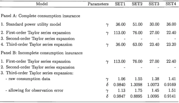
3.3.2 Estimation of the Conditional Expectation of Consumption 90 3.3.3 Required Order of a Taylor Series Expansion 91 3.3.4 The Hansen-Jagannathan Volatility Bound Analysis 92
3.3.5 Model Calibration 97
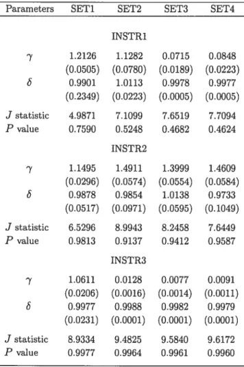
3.3.6 GMM Results 100
3.4 Concluding Remarks 101
4 An Empirical Assessment of a Consumption CAPM with a Reference Level under
Incomplete Consumption Insurance 114
4.1 Introduction 114
4.2 The Equilibrium Multifactor Pricing Model 116
4.3 Preferences 118
4.4 Empirical Analysis 125
4.4.1 Description of the Data 125
4.4.2 The Estimation Methodology 128
4.4.3 Estimation Results 130
Remerciements
J’adresse mes remerciements à mes directeurs de thèse: René Garcia et Éric Renault. La confiance qu’ils m’ont témoignée, le temps qu’ils m’ont consacré et les précieux conseils qu’ils m’ont donnés tout au long de mes travaux, ainsi que leur générosité et leurs qualités humaines extraordinaires, m’ont largement aidé à mener à bien cette thèse.
Je tiens à remercier le centre interuniversit aire de recherche en économie quantitative (CIREQ) et le centre interuniversitaire de recherche en analyse des organisations (CIRANO) pour leur support financier.
Ma gratitude, également, à tous ceux qui m’ont soutenu, et plus particulièrement ma femme Julie, mon fils Alexandre qui m’ont toujours encouragé, ainsi que mes parents Ninel et Veniamin qui m’ont appris des principes dont je me servirai toute ma vie.
1.1 Introduction
The canonical consumption-based capital asset pricing model (CCAPM) where a repre sentative agent maximizes his expected time-separable utility over uncertain streams of consumption is the workhorse of financiai economists. It allows to understand intuitiveiy the marginal utility trade-offs between different time periods or states of nature given some specification of the agent preferences. After ail, consumption is what individuais ultimately care about and it shouid be refiected in their valuation of assets. However, when per capita consumption enters a power utility function, the model delivers gross inconsistencies with the observed asset returns, whether the empirical assessment is based on calibration or on formal estimation. This resilient empirical misfit lias triggered, over the last two decades, a long series of attempts to modify the basic model in order to achieve empirical success.
À useful way to summarize the various directions in which preferences have been enriclied is to consjder that a state variable needs to be added to the basic model. This variable could be a benchmark level of consumption, as in the rich literature on habit formation. The main idea of the habit formation approach is that an investor derives utility not from the absolute level of consumption but from its level relative to a benchmark which is related to past consumption (Abel (1990, 1996), Campbell and Cochrane (1999), Constantinides (1990), Ferson and Constantinides (1991), Heaton (1995), and Sundaresan (1989)). When this reference level depends on past aggregate consumption, the catching up with the Joneses specification of Abel (1990), it captures the idea that the individual wants to maintain lis relative status in the economy. The relative social standing is aiso present in the specification expiored by Bakshj and Chen (1996) where absolute or relative wealth besides consumption determines utility.
Recently, Abel (1999) lias generalized this specification by making the benchmark level of consumption a function of current as well as recent levels of consumption per capita. It also generalizes Gali’s (1994) specification of consumption externalities whereby agents have preferences defined over their own consumption as well as current per capita consumption in the economy. They want to keep zip with the Joneses. In ail these specifications where the state variable is contemporaneous with consumption, it is noteworthy to emphasize that
there is a separation between the attitudes towards risk and intertemporal substitution even though the agent maximizes expected time-separable utility. Indeed, this separation is generally associated with the non-expected utility framework of Epstein and Zin (1989) where the agent combines his current consumption with expected future utility in a recursive way.
In the model proposed in this paper, we maintain the representative agent paradigm as well as the time-separable expected utility framework. Our agent derives utility both from the level of consumption relative to a state variable which we eau the reference level and from the absolute value of this reference level, that is U(,
$)
in ratio form or U(C—S,$t)in difference form. Such a consumer-investor will use assets to smooth not only fluctua tions in the position of consumption with respect to a benchmark level of consumption but also movements in this benchmark level. At the most general level, this benchmark consumption provides a way to extend the intertemporal choice of consumption without uncertainty to risky consumption streams. When no uncertainty prevails, the future levels of reference or benchmark consumption, when seen at time t, coincide with the optimal future consumption values, that is St+h = C11, identically for h O. In a risky environ
ment, the coincidence prevails oniy in expectation and the reference level is interpreted as the benchmark consumption the agent lias in mmd when deciding lis risk-taking behavior, Et[St+h] = Et[Ct+h], for all h O. This formulation leaves open two possibilities. Either
the reference level is an expectation of future consumption given past information or it is a function of colltemporaneous information, as some macroeconomic variables which belong to the agent’s information set at time (t + h) may affect the assessment of the reference level $t+h. We will see that these two modeling avenues relate to different asset pricing
models present in the literature and have different implications for the disentangling of the elasticity of intertemporal substitution from the risk aversion coefficient.
The specification is similar to the general formulation in Abel (1990) and was recently used in a saving and growth model by Carroil, Overland, and Weil (2000). This allows to test formally if the absolute level of per capita consumption is important per itself for pricing assets, over and above consumption relative to the reference level as it is specifled in the habit formation models of Campbell and Cochrane (1999) and Constantinides (1990). However, contrary to these habit formation specifications, we do not limit the reference
level to depend solely on consumption, past or current. Indeed, it can be a function of other variables such as wealth (value of the market portfolio) and we then recover a speci fication similar to Bakshi alld Chen (1996). The novelty ofoui approach is apparent when the reference level is made a function of both past consumption and the value of the market portfolio since we obtain a stochastic discount factor (SDF) which embeds the usual habit formation approach together with the so-called Kreps-Porteus specification of the recursive framework of Epstein and Zin (1989). When we estimate this new specification with ag gregate per capita real consumption and returns on the value-weighted CRSP stock index or size portfolios, we obtaill economically plausible values for the parameters, contrary to either the habit formation specification or the Epstein-Zin approach taken separately.
Saying that the future levels of S are equal in expectation to the future levels of con sumption means that S, represents the permanent component of consumption. Allowing $ to depend on variables other than consumption is suggested by the resuits of Alvarez and Jermann (2002) who show that the size of the permanent component in consumption obtained from coilsumption data alone is much lower than the size of the permanent com ponent of pricing kernels. Therefore, they recommend that in representative asset pricing
models preferences should be such as to magnify the size of the permanent component in consumption. The modeling of our reference level will do just that. When the reference level is made a function of the value of the market portfolio, another permanent component is added to the prici;ig kernel. In the latter formulation, the consumption weaÏth ratio will enter the pricing kernel. Lettau and Ludvigson (2001) have emphasized the promillent role played by the log consumption-wealth ratio as a conditioning variable for improving the performance of unconditional specifications.
Another important feature of oui approacli is to add a moment condition to the set of asset pricing moment conditions. This additional condition relates the growth rate of log consumption to the variables deemed to characterize the growth rate of the log reference level. The estimation of this linear equation delivers an estimated value for the growth rate of the reference level which is used in the asset pricing equations. The estimatioii of the linear eqilation and the asset pricing Euler conditions can stiil be carried out jointly, imposing cross-equation restrictions which improves efficiency of the estimates of preference parameters. Recently, Neely, Roy, and Whiteman (2001) have addressed the issue of near
nonidentification of the risk aversion parameter in the intertemporal consumption capital asset pricing model. They conclude that imposing natural identifying restrictions yields sta ble estimates of the parameters. Hansen and Singleton (1983) have also added information through an equation for predicting consumption growth.
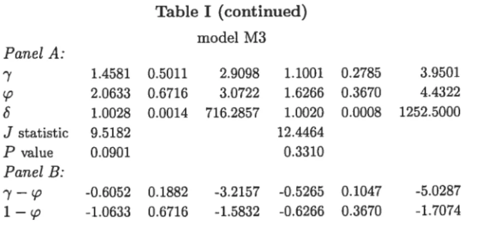
We follow this approach to estimate several generalized versions of the habit formation models. In ratio specifications, habit may depend on one lag of consumption or respond gradually to changes in consumption. In both cases, we find mild support for the presence of the reference level per itself in the utility function. Moreover, the estimates of the time discount parameter are always greater than one. We also test the specification in difference proposed by Campbell and Cochrane (1999). Contrary to the ratio models, we find strong support for the hypothesis that the absolute value of the reference level enters the utility function.
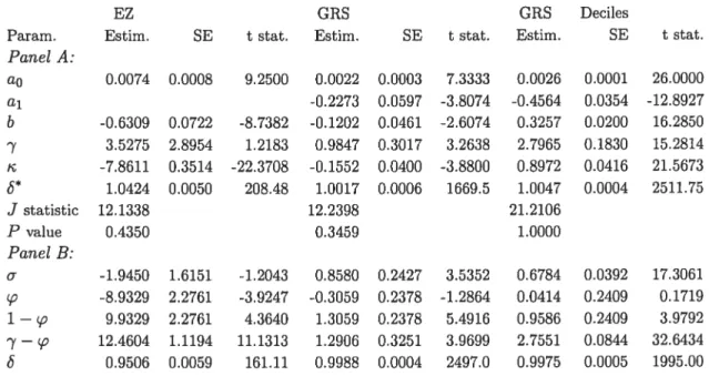
If we assume the reference level growth rate to be a function of the return on the market portfolio, our model of expected utility yields a SDF which is isomorphic in its pricing implications to the Epstein and Zin (1989, 1991) pricing kernel. A striking feature of the comparison between the Epstein and Zin (1989, 1991) non-expected utility model and expected utility model with a reference level is that the measures of risk aversion differ while the elasticity of intertemporal substitution remains the same in the two models. We explore in detail this difference in the interpretation of the risk aversion parameter in Garcia, Renault, and Semenov (2002). When we estimate this specification of our model which is observationally equivalent to the Epstein and Zin (1991) specification, we obtain a negative point estimate of the elasticity of intertemporal substitution but not significantly different from zero.
Finally, when we allow the reference level growth rate to be determined both by past consumption and by the return on the market portfolio, we obtain a SDF which incorporates habit formation in a Epstein-Zin-like SDF. With this specification, we obtain precise and reasonable estimates of the coefficient of relative risk aversion (RRA) (around 1), of the elasticity of intertemporal substitution (0.86), and of the time discount factor (0.9988).
Loss or disappointment aversion preferences have also received attention to salvage the consumption-based asset pricing model.1 Recently, Barberis, Huang, and Santos (2001)
proposed a model of time-varying risk aversion where the investor is loss averse over finan cial wealth fluctuations. Our reference level model can accommodate specifications in which the investor expresses disappointment aversion whenever lis consumption falls under the reference level. Our resuits show that for consumption above habit, the most plausible as sumption is that the representative consumer derives utility from both consumption relative to habit and the absolute level of habit. As consumption declines towards the benchmark level, we cannot reject the assumption that the conventional time- and state-separable util ity model well describes the agent’s preferences. When we test a model of loss aversion similar to Barberis, Huang, and Santos (2001), we conflrm the importance of the absolute value of the reference level in the utility function. Therefore, we are led to conclude that our utility specification not only opens new avenues for modeling the SDF but is robust to existing extensions of the standard CCAPM model.
Our approach can be put fruitfully in relation with the line of research which emphasizes stochastic prices of consumption risks and adds flexibility to the standard CCAPM through the risk aversion speciflcation.2 By allowing attitudes towards risk to reflect the information set used for consumption and savings choices, risk aversion is no longer flxed, but contingent upon the state of the world.3 The same individual may be a risk-lover over certain states of the world and risk averse over others, adjusting his tolerance to risk according to the characteristics of the problem that he faces. Such shifts in attitudes could be related to numerous factors. Bakshi and Chen (1996) and St-Amour (1993), for example, allow for wealth-dependent attitudes towards risk, when the equilibrium relative risk aversion is a decreasing function of the individual’s wealth, thus implying countercyclicality of risk aver sion. In Campbell and Cochrane (1999), Constantinides (1990), and Sundaresan (1989), who introduce time-varying prices of risk through habit formation, relative risk aversion in creases as consumption declines towards habit and, therefore, also displays a countercyclical
and Garcia (1993), and Epstein and Zin (2001) for disappointment aversion.
2One can include in this une of research Bakshi and Chen (1996), Campbell and Cochrane (1999), Chou, Engle, and Kane (1992), Constantinides (1990), Cordon and $t-Amour (1998a, 1998b), Harvey (1991), IVlark (1988), McCurdy and Morgan (1991), Melino and Yang (2003), St-Amour (1993), and Sundaresan (1989).
31n the standard power utility model, the SDF is just consumption growth raised to the power —y and, thus, one needs a large value of y to get a volatile pricing kernel. The state dependent risk aversion implies that consumption shocks generate larger unanticipated fluctuations in marginal utility than under fixed preferences and, therefore, one can instead get a volatile SDF from n volatile relative risk aversion.
pattern.
Our made! is also related ta the nanlinear pricing kernel af Dittmar (2002). Me apprax imates an unknawn marginal utility functian by a Taylar series expansian. The resulting pricing kernel is a palynamia! functian in aggregate wealth and human capital. Me further shaws that a cubic pricing kernel is necessary ta describe the data. Mawever, this pricing kernel cannat simultaneausly deliver the nanlinearity necessary ta price assets and mana tanically decrease. Our specificatian may affer the functianal farm af the pricing kernel that is missing in Dittmar (2002), which ensures that the pricing kernel is bath decreasing and potentially exhibiting a high degree af nanlinearity.
Our made! may be given an alternative interpretatian. The representative agent can be thaught as a portfalia manager whase performance is evaluated in terms of a benchmark as it is the case in practice.4 The idea of a reference level determining the utility af the investor is related ta an a!der literature. Porter (1974), Fishburn (1977), and Maithausen (1981) present a risk-return made! in which risk is assaciated with autcomes be!aw some specifled target level and return is assaciated with autcomes abave the target. A decisian maker may disp!ay variaus preference far autcames abave and belaw the target outcame. They show congruence between that made! and a specific farm af expected uti!ity function. In investment contexts, decision makers are assumed ta derive utility fram fluctuations of outcames re!ative ta some target leve! af return an investment (Green (1963), Swa!m (1966)). Malter and Dean (1971) estimated utility functions far changes in net wea!th. Our madel can be viewed as a particular extension ta a dynamic setting of that risk-return approach, when the reference leve! is seen as a target.
The rest of the paper is organized as follows. In Section 1.2, we discuss the major features of the model in which a consumer derives uti!ity from consumption relative ta some reference consumption !eve! as well as from this level itself. Section 1.3 examines the empirica! implications af the propased utility function under alternative specifications of the reference level generating process and assesses the contribution of the mode! towards explaining asset returns in US month!y data. Conclusions are presented in Section 1.4.
1.2
An Expected Utility Model with a Reference Consumption Level
We generalize the standard time-separable utility function by assumillg that each consumer derives utiiity from consumption relative to some reference consumption level as well as ftom this level itself:
1—7
()
s-(1)
(‘-7)(1-)
where -y is the curvature parameter for relative consumption, C is current consumption, $ is a time-varying reference consumption level, and the parameter p controls the curvature of utility over this benchmark level. If p = -y, we get the standard time-separable power utility
function (the reference consumption level plays no role in asset pricing). With p = 1, we
obtain a preference specification where the ratio of the agent’s consumption to the reference consumption level is ah that matters. If p ‘y and 1, then the agent takes account of both the ratio of his consumption to the subsistence level and this level itself when choosing how much to coilsume. Then, when maximizing expected utility over an infinite horizon, the agent assesses:
= [(1 -‘y)(l
- )]1 6hE [(±h)
‘
su].
(2)We consider that the reference level $t is external to the agent and E denotes n condi
tional expectation given the information at time t. At the most generai level, this benchmark for consumption provides a way to extend intertemporal choice of consumption without un certainty to risky consumption streams. When no uncertainty prevails, the future sequence of the reference level at time t, 8t+h, h O, coincides with the optimal future consumption
values:
= Ct identicaHy for h 0. (3)
In a risky environmellt, we just generalize condition (3) in terms of conditional expec tations:
= Et[Ct+h] for ail h 0. (4)
Therefore, we can interpret as the reference level the agent has in mmd at time t to decide his risk-taking behavior. In the latter case, some macroeconomic variables which be long to the agent’s information set at time (t +h) may affect the assessment of the reference
level This specification is very general since the reference level remains unspecified. One can see however that several models in the asset pricing literature appear as particular cases of this general utility functiori. It is the case of the furictional form considered by Abel (1990). This specification is obtained with -y = p and St
= [Gji D]J where
t
denotes aggregate per capita consumption. For D = 0, this is the relative consumption
model called “catching up with the Joneses”, whereas when D = 1, the individual considers
as a benchmark his own past consumption. This is the habit formation model. More gen eral models of habit cari also be envisioned. Also, one can start with a utility specification
• • . • (Ct—St)’S’—1
in differeilce instead of ratio and postulate t = 1 and cover the vanous specifications of the habit formation models in difference used by Campbell and Cochrane (1999) and Constantinides (1990) among others. Ah asset pricing models with habit for mation have imposed the constraint = 1. Recently, Carroli, Overland, and Weil (2000)
and Fuhrer (2000) have relaxed this constraint and expiored the ensuing implications in saving and growth model. They found that such a specification could expiain that saving and growth were strongly positively correlated. It appears therefore worthwhile to allow to be different from 1 and to formally test the constraint cp = 1 in asset pricing models with
habit.
The wealth-induced status model of Bakshi and Chen (1996) is another particular case of this specification. Ail models proposed in their paper cari be formally expressed with a utility function conformable to (1), whether S is simply the weaith W of the individual or the wealth relative to the wealth of their reference group V. However, since our consumer cares about consumption relative to the reference level, our interpretation of this model will be different. Take the case where $t is W. Our model tells us that the individual makes his consumption and portfolio decisions according to his consumptioll-wealth ratio, and not consumption per se, as well as his level of wealth. In this sense, we incorporate a variable in the model which is important in pricing assets as demonstrated by Lettau and Ludvigson (2001). As we will stress below, the SDF which resuits from such a specification of the reference level is closely related to the SDF of Epstein and Zin (1989).
Before we discuss in detail the various strategies for modeling the reference level of consumption in relation to the existing asset pricing models and possible extensions of these models, we need to estabhish how the presence of this level will change the risk premia
and the intertemporal consumption trade-offs.
Since the reference level is collsidered external, the marginal utility of consumption is given by
= CS. (5)
Then, when maximizing his expected utility over an infinite horizon, the investor will choose an optimal consumption profile which will satisfy the following Euler equations:
E
[
(‘)
= 1, = (6)where I is the number of assets considered and Rj,+i is the gross return ofasset i from t to t + 1. Expectations in (6) are taken conditionally on information available to the individual in period t and Rj is the gross return on asset i. The SDF is then
/r \Y /c \7°
cl’’t+l ‘ (‘t+1
JVit+1OL—) 1——
\L’t/ \
To discuss the implications of asset pricing models, it is common to assume joint condi tional lognormality alld homoscedasticity of the consumption growth rate and asset returus, since we obtain loglinear relations for asset returns. With our utility model, the risk-free rate will be determined by the following equation:
Tf,t+1 = —log6 + 7Et [Ct+1]
—
—(—
)E[St+i]—
(
—
)22+—
(8)whereas the risk premium on any asset i will be given by:
Et [ri,t+i
—
Tf,t+1] = —u +— ( — )
Ui8, (9) where ct+i S the log of the consumption growth rate, is the log of the reference consumption level growth rate, is the log of the simple gross return on asset i, and o denotes generically the unconditional covariance of innovations.The first three terms on the right-hand side of (8) and the first two terms on the right hand side of (9) are the same as for a time-separable power utility function of consumption alone. Thus, utility function (1) can help to explain the risk-free rate puzzle if the term
puzzle if the term — Q-y
— y) oj is positive. Therefore, the position of y with respect to y
and the signs of the covariances between the innovations in the reference level growth rate and the innovations in consumption growth and in asset returns are key in solving the two puzzles.
Another important dimension over which the resolution of the puzzles is discussed is the disentangling of risk aversion and intertemporal substitution. The standard consumption CAPM model with power utility imposes a functional restriction which is not sustainable theoretically nor supported empirically. For our mode!, we can study this separation by writirig the expected return equatioll, aiways under the same joint conditiollal !ognormality and homoscedasticity of the consumption growth rate and asset returns:
E [r,t+i] = —loge + 7Et [Ct+1]
— 122 —
(
— y)E [st+y] —(
— )2 +(
— y)cs — +7Jic —(
— y)ais. (10)To study intertempora! substitution in a simplified framework, let us assume that ah quantities are now deterministic so we can ignore the expectation operators. With the standard power utility function under this assumption, equation (10) reduces to
Tt+1 = —log6 + 7Cji — _-y22 (11)
1 which implies u =
=
. From (10), it fol!ows that when the agent s preferences are
of the form (1), the intertemporal elasticity of consumption is 1 + (7— y) ‘
(12)
7
where
8rt+1 can be rnterpreted as the elasticity of the reference level with respect to the
interest rate.5 The latter equation implies that the elasticity of intertemporal substitution differs from the inverse of the RRA coefficient if Q-y — y)
8,9
0. In our external reference level setting, it will therefore be important to distinguish the specifications where this leve! depends on past variables, in which case the disentang!ing will not occur, from
5As we can see from equations (9) and (12), since the terms and u have the same sign, if utility model (1) generates anequity premiumwhich is larger than that produced by the basic power utility
model, it also generates an elasticity of interteniporal substitution which is less than the inverse of the RRA coefficient.
the ones where it depends on contemporary variables and allows to differentiate o- from the inverse of -y.6 This justifies to analyze these specifications under two separate subsections under these headings.
Finally, the poor empirical performance of the standard consumption CAPIVI model lias led researchers to explore specifications with a kink in tlie utility function, preferences changillg above and below a certain threshold. Benartzi and Thaler (1995) examine single period portfolio choice for a loss averse investor, which means that gains and losses will not receive the same weight in terms of utility. Bonomo and Garcia (1993) and Bekaert, Hodrick, and Marshall (1997) have explored the asset pricing implications of a related but different type of preference called disappointment aversion, introduced by Epstein and Zin (1989) in n recursive utility framework.7 Recently, Barberis, Huang, and Santos (2001) proposed an asset pricing model where the investor is loss averse over financial wealth fluctuations. Given that our model introduces a reference level, it is natural to extend our investigation to specifications where preferences will be different above and below tlie reference level. When the latter will be related to past consumption variables, we will be able to test generalizations of the habit formation or catching up with the Joneses models. V,Tlien it will 5e related to financial wealth, we will provide tests of models similar to the loss aversion model of Barberis, Huang, and Santos (2001). The discussion of these various specifications wiIl be the object of the third subsection.
1.2.1 Reference Level Determined by Past Variables
In this subsection we will model the reference level strictly as a function of the past variables. This will allow us to make the link witli the habit formation literature and discuss liow this model lias tlie potential to extend it. We will also discuss tlie persistence of the reference level and an estimation strategy.
6Ferson and Constantinides (1991) study an internai habit model, in which the utility is a power function of the difference between t,he current consumption flow and a fraction of a weighted sum of ]agged consump tion flows, and prove that habit persistence and/or dmabiiity of consumption drive a tvedge between the elasticity of consumption with respect to investment returns and the inverse of theRRAcoefficient.
TPreferences that exhibit disappointment aversion have been axiomatized by Gui (1991) to offer a solution to the so-called Allais paradox.
Modeling of the Reference Level. An approach commonly used in the literature consists in assiiming that the reference consumption level, St+i, is an expectation of consumption Ct1 taken conditionally on past consumption levels, that is = E [C+1
ICt,
Ct_1,...].8This is based on the idea that tomorrow’s marginal utility of consumption is an increasing function of today’s consumption. According to this approach, the time-varying subsistence level, or habit, can be specified either as an internai habit (habit depends on agent’s own consumption) (Constantinides (1990), Sundaresan (1989)) or an external habit (the mdi vidual’s reference consumption level depends on aggregate consumption, which is assumed to be unaffected by any one agent’s consumption decisions, rather than on the history of individuai’s own consumption) (Abei, 1990, 1996, Campbeii and Cochrane, 1999).
Let us suppose that $t = C1, as in Abel (1990). As already mentioned, the ratio
habit-formation model or the catching up with the Joneses are special cases of (1) when
f
= 1. The utility function is in this case: Ut
= \Ct_i)
, with c = O giving the standard
time-separable model and c = 1 the catching up with the Joneses modeL In the latter case,
only relative consumption matters to the consumer.
Recently, Carroll, Overland, and Weil (2000) and Fuhrer (2000) have argued that one need not impose the constraint that a has to be O or 1. For values of c between O and 1, both the absolute and relative consumption levels are important to the consumer. The way we have rewritten the utility function lends itself to a different interpretation. A good way to start is to suppose that actual consumption neyer deviates from the reference level. In this case there is no consumption risk and the consumer needs just decide how to intertemporally substitute consumption over time. The exponent of the reference ievei is then quite naturaliy p = 1 — , with the elasticity of intertemporal substitution u
0f course, there is consumption risk and the consumer reacts to it trough the curvature parameter which measures risk aversion. Therefore, this specification offers potentiaily a natural disentangling between risk aversion and intertemporal substitution. We will explore this aspect in the next subsection since this disentangling cannot occur when the reference level depends on past aggregate consumption =
o).
Since, according to the habit formation approach, the reference consumption level$t is supposed to depend on past information only, we are allowed to assume that it should be
known to an agent at time t. Given this reasoning, we propose to use the following two-stage estimation procedure. In a first stage, we estimate the subsistence level under a particular assumption about the benchmark level formation process. In a second stage, we estimate the Euler equations (6) with the reference consumption level replaced with its estimate obtained in a first stage. Using this approach allows us to estimate a model exploiting the two specifications mentioned above whereby the stock of habit is assumed to be a function of lagged levels of consumption and the parameter which indexes the importance of the reference consumption level is added in the utility function. Given this two-stage estimation procedure, throughout the remainder of this section, we focus flot only on the nature of the benchmark level generating process, but also on how this reference level can be estimated.
Persistence of the Reference Level and Estimation Strategy. The persistence of the reference level formation process is an important issue for consumption-based asset pricing models. Alvarez and Jermann (2002) derive a lower bound for the size of the permanent component of asset pricing kernels and find that it is very large. They also show that in the many instances where the pricing kernel is a function of consumption, innovations to consumption must have permanent effects.
As we have seen in the last section, a number of papers have assumed that habit de-pends on only one lag of consumption. An alternative view is that the subsistence level responds only gradually to changes in consumption (Campbell and Cochrarie (1999), Car roli, Overland, and Weil (2000), Constantinides (1990), Fuhrer (2000), Heaton (1995), and Sundaresan (1989)). Carroil, Overland, and Weil (2000), Constantinides (1990), and Fuhrer (2000), for example, assume that the benchmark level evolves according to the adaptive pectations hypothesis, which postulates that the change in expectations, S+i— St, is equal
to a proportion À of Ïast period’s error in expectations, G — S. That is,
S+i—S=À(C—S), 0À1 (13)
or, equivalently,
In this paper, we consider the unrestricted form of (14):
St+ =a+ÀC+(1—À)$, (15)
whereas the adaptive expectations hypothesis postulates a = 0.
To replace the unobservable expected consumption, St, in equation (15) with an observ able variable, we repeatedly lag and substitute equation (15) to obtain
= + À (1
—
À)C_ (16)which means that the habit stock is a weighted average of part consumption flows with the weights À(1
—
À) declining geometrically with time.Since the subsistence level, St+i, is assumed to be an expectation of consumption taken conditionally on past consumption levels, we can rewrite (16) as
= + À (1
—
À)C_ +Et+1, (17)where e is an innovation in C+1.
Using the habit formation approach to modeling the reference consumption level allows us to determine whether habit persistence in preferences or durability in consumption ex penditures is dominant. Habit persistence in preferences implies that today’s consumption har a positive effect on tomorrow’s marginal utility of consumption: ac_1 > 0. for
utility function (1), ac_1 = (Y
—
ço) Hence, if (y—)
‘T >habit persistence dominates durability. If
(
—
)
< 0, then the effect of durability is dominant.When Alvarez and Jermann (2002) measure the size of the permanent component of consumption using only consumption data, they find it is well lower than the size of the permanent component of pricing kernels. They suggest that in a representative agent asset pricing framework the specification of preferences should magnify the permanent component in consiimption. The reference level inouiutility function offers a way to introduce variables which, along with consumption, will contribute to amplify the permanent component of the asset pricing kernel. We will explore these possibilities in the next section where we will most notably look at the link between the reference level and the return on the market portfolio.
1.2.2 Reference Level Determined by Contemporaneous State Variables
A more general approach to modeling the subsistence level formation process is to assume that an agent can take into account not only the information available to him at timet, but also some information availabie at time t+1, when lie forms lis reference consumption level,
$t+i. Abel (1999) and Cochrane (2001), for example, suppose that the agent’s benchmark
level depends on current period aggregate consumption. Campbell and Cochrane (1999) also make their habit a contemporaneous variable.
According to (6), the reference consumption tevel growth rate is ail we need to know about the reference ievei for asset pricing. We first motivate by an economic argument why the reference ievei growth rate should be made a function of the return of the market portfolio. We then present a general framework which allows other contemporaneous or past state variables to expiain the reference ievel growtli rate. We further show how to nest in this framework both the Epstein and Zin (1989, 1991) pricing kernel and the power utiiity model of Campbeli and Cochrane (1999) with a slow-moving externai habit.
Modeling the Growth Rate of the Reference Consumption Level. The SDF defined in (7) implies that the reference levei must produce conditional expectations which not oniy are constrained by (4) but also are consistent with asset prices. Let us consider first the market portfolio pricing condition. If we denote by RM,t+1 the gross return on the market portfoho observed at time (t + 1), we get
/C+ (St+iN7
6 I L RM,t+1 = 1. (18)
\L’tJ \t]
Condition (18) shows that covariation between the reference levei and the market return may compensate for the lack of covariation between consumption and the market return. This extension of the traditional consumption-based asset pricing model may help to solve severai asset pricing puzzles features associated with aggregate data. As stressed by Bar beris, Huang, and Santos (2001), such an extension has some behavioral foundations since it captures the idea that the degree of loss aversion of the investor depends on his prior investment performance. To make even more explicit this tiglit reiationship between the reference level and investment performance as measured by the market return, we will re fer to a loglinearization of conditionai moment restrictions (4) and (18) (see Epstein and
Zin (1991) for similar interpretations based on a loglinearization of the Euler equations). Conditional expectations are computed as if the vector
(Ct+1,zSt+1,TM,t+1) = (109
()
,tog()
to9RMt+1) (19)were jointly normal and homoscedastic given the information available at time t. Conditions (4) and (18) at horizon 1 become:
— Et[st+i]
= ,çi, (20)
—7Et[ct+l] + (‘y —o)Et[1st+i] + Et[TM,t+11 = (21)
for some constants k1and 2. Equivalently, these two restrictions say that both [8t+1 — Ct+1] and [St+i—TM,t+1] must be unpredictable at time t. The Epstein and Zin (1989)
pricing model is in fact observationally equivalent to the particular case of our CCAPM with reference level where [st+i — is not only unpredictable but constant:
1
= —T1I,t+1 + (22)
for some constant i. In other words, we consider the particular case where the benchmark growth rate of consumption is loglinearly determined by the current value of the market return, with a siope parameter equal to the elasticity of intertemporal substitution. Note that this is in accordance with the portfolio separation property generally implied by ho rnotheticity of preferences (see Epstein and Zin, 1989), whereby optimal consumption is determined in a second stage, after the portfolio choice has been made.
An interesting generalization is to relate the log of reference level growth to past period consumption growth, as we did in the previous section for habit formation models, and the current period return on the market portfolio in the following way:
= ao + x Act+i_j +b X (23)
9This assumption also relates oui framework to the prospect theory of Kalineman and Tversky (1979) and Tversky and Kahneman (1992). The intuition behind this is that if the level of market portfolio moves up, an agent should think that this increase in lis wealth will bring him tIc additional consumption. It means that tIc benchrnark consumption level, whidh refiects anticipated consumption, should also move up.
Condition (20) is consistent with a model where consumption growth is equal to the reference level growth rate plus a constant and noise:
= kl +St+1 +Et+y, (24)
where e is an innovation in Lct+i with E(e+1) = O and Et[st+et+j = 0. It follows
that the log of consumption growth may be described by an affine regression
=ao + ‘ + a x Act+;_ + b X TM,t+; + (25)
with Et [TM,t+Et+1] = 0. From (23),
n
f L’t+1i \ b
= A
L
J
(Ri,+;) , (26)i=1 t—i]
where A exp (ao).
Under the above assumptions, the SDF (7) becomes
c
c
aQy—çL)=
(&!)
(
-‘—)
(RM,t+l)’°, (27) where 6 6A°. This specification allows to separate risk aversion from intertemporal substitution, since 1+b(7—’) Therefore, we may rewrite (27) asn aj(7—)
=
6*
(±.)
H
(Gt+i) (RM,t+l)’,(28)
where F u’y — 1, so that testing the nuil hypothesis H0 : = O is equivalent to testing
H0 : u
7
This specification of the SDF is interesting for several reasons. First, when a = O
(i = 1, ...,n), the SDF in (28) is isomorphic in its pricing implications to the Epstein and
Zin (1989, 1991) pricing kernel for a Kreps and Porteus (1978) certainty equivalent. When b O, the reference level growth depends only on previous period consumption growth, as in the habit formation approach. When neither of these restrictions holds, we have a new asset pricing model which will put together two strands of the literature which evolved in parallel until now.10 This new framework offers a way to test existing models since they
‘°Recently, Schroder and Skiadas (2002) have shown an isomorphism between competitive equilibrium models with utilities incorporating lineat habit formation and corresponding models without habit formation. In particular, they have offered a solution ta problems with utility that combines recursivity with habit formation.
are embedded in the general specification. Let us look in more detail at the comparison between the Epstein and Zin SDf obtained under a non-expected recursive utility model and the SDF under expected utility with a reference level.
Comparison with the Epstein-Zin Stochastic Discount Factor. Under the assumption that a = O (i = 1, ...,n), the SDf in (2$) reduces to
*fCt+1N
Mt+1 = (RM,t+1) . (29)
When ‘y = i/o- (i.e. ,ç = 0), we get the $DF for a standard power utility model. When
‘y = 0, the consumption growth rate is irrelevant to the determination of equilibrium asset
prices and the market return is sufficient for discounting asset payoffs. In any other case, both the consumption growth rate and the market return are relevant to the determination of equilibrium asset prices.
The Epstein-Zin (1989, 1991) $Df is
1—’ t \ i(p-1)
1-= ti (Ri,+i)7’, (30)
where p is the parameter reflecting intertemporal substitutability (the elasticity of intertem poral substitution is
‘J
= 1/ (1—p)) and is the risk aversion parameter. Epstein and Zin
(1989) interpret as a measure of risk aversion for comparative purposes with the degree of risk aversion increasing in c.
The observational equivalence between the SDFs (29) and (30) implies that 1 (p
— 1), and o-’y — 1 — 1. The two last identities put together yield
o- = = 1/ (1
—p) =
, that is the elasticity of intertemporal substitution in model (1) is equivalent to that in the Epstein-Zin non-expected recursive utility specification. In the case of the Epstein-Zin utility function, the elasticity of intertemporal substitution may not be equal to 1, whereas in the case of utility specification (1) any value of o- is allowed.
Since o- = 1/(1
— p), ‘y
= (1 — o-)
/
(u — 1). It follows that the measure of risk aversionin the Epstein-Zin (1989, 1991) utility specification, o-, is equal to 1 — ‘yo- +‘y. It is easy to
see that o- is equal to the RRA coefficient, ‘y, only if‘y= i/o-, what corresponds to the case
of the standard power utility model.’1 If‘y differs from i/o-, the parameter o- is no longer
“In the Epstein-Zin (1989, 1991) preference specification, the parameter c is the RRA coefficient when 1— p (in this case, we get the SDF for the conventional power utility model, for which =
the RRA coefficient and is equal to the RRA coefficient plus the term 1 —
In our model, risk aversion is defined with respect to the unpredictable discrepancy between actual consumption and the reference level (a quantity independent of the attitude towards risk) and not with respect to the forthcoming level of recursive iitility which stili mixes attitudes towards risk and intertemporal substitution. Garcia, Renault, and Semenov (2002) develops further the comparison between the two models.
The SDF in (29) yields the following Euler equations:
E [6*
(ii)
—(RAf,t+1) RiL+1] = 1, i 1,...,1.12 (31)
A test of the nul! hypothesis H0 : u = O can be carried out by testing the null hypothesis
Ho: = —1 and 0. To examine whether u 1/7, we have to test the nuil hypothesis
H0: = 0.
We may rewrite the SDF in (29) as
f Ç*
ï+i
JVlt+1 =
= (6*1/0 (1)
)
° ((R,Ït+i)_bj’ o (32)Approximating this geometric average with an arithmetic average yields
M+1 = 8
Q’io
(i)
+ (1 — O) (RM,t+1). (33)
After substituting this linear approximation into the Euler equations (31), we obtain
1 OE [6*1/0
(1)
(Rt+i)] + (1 — O) E [(RM,t+1)- (Ri,+1)]. (34)
It can be viewed from (34) that, as in the Epstein-Zin utility function case, the riskiness of an asset is measured by means of the covariance of its return with the market portfolio retirn (as in the static CAPM) and the covariance of its return with the consumption growth rate (as in the intertemporal CAPM).
Another usual to illustrate this interpretation is to assume joint lognormality and ho moscedasticity of the consumption growth rate and asset returns. Under this assumption,
‘2Since ç u-y — 1, one may want to estimate u directly. However, we prefer estimating instead of u
20
we have
E [ri,t+i — Tf,t+1] —u +7ic
— (‘y —y)boiM
= + y + (1 — 9)buM). (35)
So, the parameter y can be thought of as a coefficient measuring the contribution of a weighted combination of asset i’s covariance with consumption growth and asset i’s covariance with the market return towards the risk premium on asset i.
Alvarez and Jermann (2002) refer to the recursive preferences of Epstein and Zin (1989) and Weil (1989) as a way to increase the size of the permanent component in the pricing kernel. Our utility specification, through the assumed connection between the reference level and the value of the market portfolio, adds similarly a permanent component to the pricing kernel.
Habit Formation in DifFerence with a Reference Level. Campbelland Cochrane (1999) interpretation of the reference level $t as an external habit leads them to specify sorne nonhinear dynamics consistent with the structural restriction St < Ct. Actually they specify the surplus consumption Ht CSt as a conditionally lognormal process. In this setting, we can still introduce our reference level principle by considering that the representa.tive consumer derives utility from consumption relative to his reference level as well as from this level itself
e-il—7 q7—
L’t ‘t Ut—
(1—’y)(l—y)
according to (1). However, in order to really nest Campbell and Cochrane (1999) utility model, we must extend this formulation by writing
—
lit —
(1—7)(1—y)
Then, testing H0 : -y = y amounts to testing the particular case of Campbell and
Cochrane (1999) utility model. At first sight, it may appear a bit artificial ta introduce three variables in the definition of the utility functions since any of them is a well-defined function of the two other ones. However, the utility function rewritten in that way (37) helps to better understand the external habit paradigm of Campbell and Cochrane (1999). The statistical model (see (40) below) specifies the joint dynamics of the two lognormal processes (Ce, Ht) while the dynamics of the reference level St is only a by-product. However, in the
economic model, the optimizing agent considers the product (CHt) as its optimal control variable given the external habit level St. Therefore, the resulting $DF is:
(Ht+iN (C17 ($t+iN
= 6
ijff)
J]
(38)Another way to understand this formula is to realize that the utility function in (37) can also be written
(C—
(39) (1—7)(1—2)
and the consumer see the reference level $ as external.
The statistical model proposed by Campbell and Cochrane (1999) is specified in order to make the volatility of the $Df stochastically time-varying with the business cycle pattern. The consumption process is seen as a lognormal random walk while the log H pro cess has the same standardized innovation but evolves as a heteroscedastic AR(1):
c1 =g + Vt+1, Vt+1 i.i.d. N(0,u2), (40)
h+i = (1 —
)7
+ çbh + )(h)v+i.We are going to use the sensitivity function )(h) proposed by Campbell and Cochrane (1999), that is:
— 2(h
)
1 if h hmax(41)
t
O otherwise,where hmax + —
and
7Ï
= By choosing this sensitivity function,Campbell and Cochrane (1999) had two objectives in mmd. The first was to obtain a constant risk-free rate. This restriction is typically relaxed in ourmore general setting with
, where the absolute value of the reference level plays an independent role in the
utility function. The second one was to ensure that the elasticity of the reference level with respect to consumption is zero in the steady state and is a U-shaped function of h around h =
].
This objective is stiil achieved in our setting.Besides allowing for a time-varying risk-free interest rate, oui setting with y disen tangles the relative risk aversion coefficient and the elasticity of intertemporal substitution,
as already emphasized in the Epstein-Zin-like interpretation of our mode! in the previous section. This diseiltangling appears important since iII the Campbell and Cochrane (1999) mode! risk aversion
(-)
can become very large in the states of the economy where H approaches zero, that is when consumption comes very close to the externa! habit. In our setting, a large risk aversion does not automatically imply a dramatically low level for the e!asticity of intertemporal substitution. However, as in Campbell and Cochrane (1999), we make the steady state of the reference level (and in turn the sensitivity function) depend on the preferences only through the risk aversion parameter ‘y. The issue of a possible ad ditional role of the parameter in the steady state of the reference level and the sensitivity function is left for future research.Campbell and Cochrane calibrated the parameters in order to assess the mode! implica tions for asset pricing. Suppose we wanted to estimate this model and test their specification against the more general SDF (38). We shou!d be able to compute the time series of surplus consumption H and to deduce the time series of the growth rate of the reference !evel S. For the former, given and a process for consumption growth, we need the parameter 5. In choosing parameters, Campbell and Cochrane match to the seria! correlation of the log price-dividend ratio. But this measure of persistence is tightly related to the persistence of the market portfo!io return since one can always write
1ogRM, = ct+1+ tog(1 + Qt+i) — logQt, (42)
where RM,t+1 = Pt+i+Ct+i and = denotes the price-dividend ratio for a daim on
aggregate consumption. Therefore, approximately
+tog(Qt+i)
—
togQ. (43)When is viewed as a white noise (as in Campbell and Cochrane (1999)), the dynamics of the rate of growth of the price dividend ratio is tight!y related to the one of the market returil. In other words, plugging into the SDF (38) a rate of growth of the reference leve! that mimics the price dividend ratio dynamics is very similar in spirit to the Epstein and Zin SDF, as revisited in the previous subsection. In this sense, we can daim that our proposed extension of Campbell and Cochrane (1999) nests the Epstein and Zin (1989) asset pricing mode! expressed with a habit formation model in difference. Therefore, as with the
ratio model in Section 1.2.2, we maintairi habit formation preferences while disentangling risk aversion from intertemporal substitution in a way observationally equivalent to Epstein and Zin (1989).
1.2.3 Preferences with a Reference Level as a Threshold
Introducing a kink in the utility function has been another way to attempt rescuing the consumption CAPM. Disappointment aversion and loss aversion are two examples of such preferences, the former being deflned over intertemporal consumption streams, the latter over wealth. A disappointment averse consumer will put more weight on bad outcomes than on good ones, where bad and good are deflned with reference to a certainty equivalent measure of a consumption gamble. Epstein and Zin (1989) integrate these generalized preferences in an intertemporal asset pricing model within a recursive utility framework. Bekaert, Hodrick, and Marshall (1997), Bonomo and Garcia (1993), and Epstein and Zin (2001) explore the asset pricing implications of disappointment aversion. Benartzi and Thaler (1995) also adopt asymmetric preferences over good and bad resuits, but instead of using an intertemporal asset pricing framework with preferences deflned over consumption streams, they start from preferences deflned over one-period returns based on Kahneman and Tversky (1979)’s prospect theory of choice. The central idea of prospect theory is that an investor is assumed to derive utility from fluctuations in the value of his financial wealth and to be loss averse over these fluctuations, meaning that he is distinctly more sensitive to reductions in his financial wealth than to increases. Recently, Barberis, Huang, and Santos (2001) have studied asset prices in the context of prospect theory. In their model, investors derive utility both from consumption and changes in the value of their financial wealth. They introduce loss aversion over financial wealth fluctuations and allow the degree of loss aversion to be affected by prior investment performance.
The utility function deflned in (1) offers at least two ways to model asymmetric pref erences. First, we can use the reference consumption level S as a threshold below which outcomes are penalized in terms of utility. In this generalization of habit formation models,
investors will have the following utility function:
f
J
\S/ if C Ut = ()l_Y2si_%21 . (44I
. otherwise,where .\ is a disappointrnent aversion coefficient. The intuition here is that the investor is likely to be disappointed if his consumption is lower than the reference level and, conversely, satisfied otherwise.
A second type of asymmetry could be built by modeling the threshold level in a fashion similar to Barberis, Huang, and Santos (2001). The reference level S in this case could 5e assimilated to the value of the market portfolio, whule the threshold will be given by the position of the return on the market portfolio with respect to the safe asset return. Such a utility specification yields the following SDF:
Mt+i
= +À(zt)C2 (1 — I[RM+JZRf+1])
(45)
+ ÀC22 (1 —
where RAI,t is the return on the market portfolio, Rf,t+1 is the risk-free interest rate, V+i
is the value of market portfolio, and Ir 1 is the indicator function, which takes
1RAJ,t+1ztRft+1J
the value 1 ifRAI,t+1 ZtRf,t+1 and O otherwise. The variable Zt measures the size of prior losses. The larger the prior losses, the more painful subsequent losses vil1 5e. Our goal will be to estimate such models by the generalized method of moments to assess the presence of such preferences in the data, as opposed to the calibration exercise of Barberis, Huang, and Santos (2001).
1.3
Empirical Results for Alternative Models of the Reference Level
In this section, we estimate the models described in Section 1.2 using US monthly data. After a brief description of the data construction, we discuss the estimation procedure in light of the identification issues surrounding the preference parameters. We then start by providïng the empirical resuits corresponding to the conventional time- and state-separable preferences. This will provide a basis with which to compare the richer specifications offered by the three types of models with a reference level discussed in Section 1.2. First, we estimate models for the augmented habit formation approach, where the absolute value of the reference level enters in the utility function along with relative consumption. Second, we
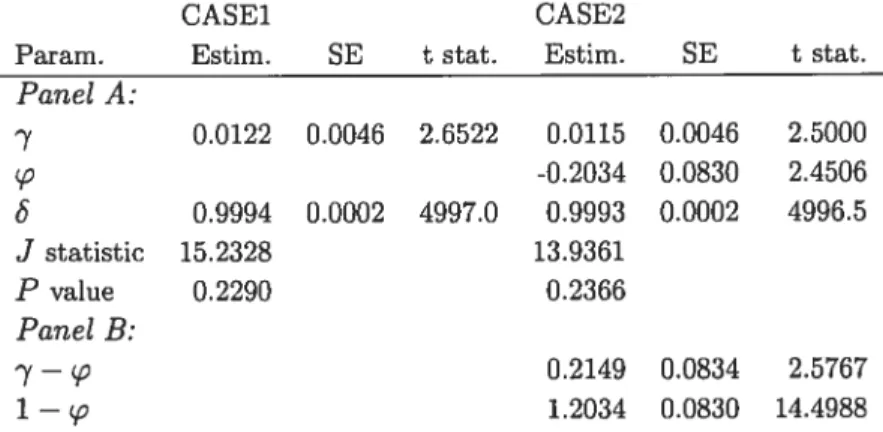
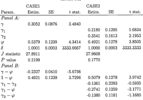
consider several specifications where the market portfolio return enters in the determination cf the reference level growth rate. We estimate models which embed two well-known models: the Campbell and Cochrane (1999) habit formation model and the Epstein and Zin (1989, 1991) non-expected recursive utility model. For the former case, instead of calibrating the model, we estimate and test the model in a GMM framework keeping the original specification cf the consumptidn surplus dynamics. For the latter, we estimate a utility specification where the reference consumption level growth rate is assumed te depend on the previous period consumption growth rates and the return on the market portfolio. As the Epstein-Zin model is seen te be a mixture cf the CAPM and the CCAPM models, this generalized speciflcation can 5e described as a ccmbination cf the CAPM with a habit formation CCAPM model. Finally, we estimate models cf asymmetric preferences, where the jnvestor draws different utilities above and below the reference level or some function cf it. Most notably, we estimate a model of loss aversion very similar in spirit te the model cf Barberis, Huang, and Santos (2001), thereby prcviding a useful ccmplemellt te their calibration whereas their model was simply calibrated.
1.3.1 Data and Estimation Issues
Consumption and Returns Data. Themeasure cf realaggregate consumption used in this paper is the personal coilsumption expenditures (in constant 1987 dollars) on nondurables and services (NDS) taken frcm the United States National Income and Product Accounts.13 Monthly per capita consumption is obtained by dividing the real aggregate consumption by the total population, including armed forces overseas.14
The nominal, monthly risk-free rate cf interest is the one-month Treasury bill return from the Center for Research in Security Prices (CRSP) cf the University of Chicago. The real risk-free rate is calculated as the nominal risk-free rate, divided by the one-mcnth inflation rate, based on the deflatcr deflned for NDS cousumpticn. As a proxy fer the nominal, mcnthly market return, we take the value-weighted aggregate nominal, monthly return (capital gain plus dividends) on ah stocks listed on the NYSE and AMEX, obtained from CRSP. The real, mcnthly market return is calculated as the nominal market return,
13Taken from CITIBASE,mnemonicsCMCNQ and GMCSQ.