Adaptive trajectory targeting within a 6-DOF simulation

Adaptive Trajectory Targeting within a 6-DOF Simulation

by

Alan Thomas

B.S., Aero/Astro Engineering

Massachusetts Institute of Technology, 1994

Submitted to the Department of Aeronautical and Astronautical Engineering in Partial Fulfillment of the Requirements for the Degree of

MASTER OF SCIENCE in Engineering at the

Massachusetts Institute of Technology

1995 Alan P. Thomas

All rights reserved

The author hereby grants to MIT permission to reproduce and to distribute publicly paper and electronic copies of this thesis

document in whole or in part.

Signature of A uthor .../... Department of Aeronautics and Astronautics

May 17,1995

C ertified by ... ...r ... ....-... Wallace Vander Velde Professor of Aeronautics and Astronautics at MIT Thesis Supervisor

A ccepted by ... _{... ...} ... .. ... MASSACHUSETTS INSTIWartmental Committee on Graduate Studies

"JUL

07 1995

ADAPTIVE TRAJECTORY TARGETING WITHIN A 6-DOF SIMULATION

by

Alan Thomas

Submitted to the Department of Aeronautics and Astronautics on May 17, 1995 in partial fulfillment of the requirements for the Degree of Master of Science in Aeronautics and Astronautics Engineering

ABSTRACT

A targeting program was coded, debugged, and tested for the CENTAUR

vehicle built by Martin Marietta. A full-up 6 degree-of-freedom (DOF)

simulation was used, along with the NLP2 optimizer built by John Betts and Wayne Hallman. The targeting program integrated almost all the real on-board computer software modules, as well as dynamic models that encompass all trajectory pertinent effects. Transfer orbit parameters were used as inputs to the optimizer in order to solve for the fuel consumption minimized trajectory. By incorporating the guidance software modules, the targeting program adjusts the transfer orbit while optimizing, which in turn alters the encompassing burns.

The targeting program was tested using the CENTAUR TC-17 mission. A comparison of the solution's transfer and final orbit parameters between this

6-DOF targeting program and a more traditional 3-DOF finite burn approach

is provided. An estimate of the targeting program's efficiency is provided as well. Results are discussed, and future recommendations are proposed.

Professor Wallace Vander Velde Thesis Supervisor:

ACKNOWLEDGEMENTS

First and foremost, I would like to thank Steve Dunham for his mentorship and major contributions to the flight simulation. Second, I would like to thank Professor Wallace Vander Velde for his advice and help. Third, I wish to thank Dr. Nikolas Bletsos for his support and guidance. Also,

gratitude is offered to John Betts and Wayne Hallman whose NLP2 optimizer is essential to the targeting program. I would like to thank Tom Morgan for his help in understanding the intricacies of the proconsul program. Finally, I wish to mention Andrew Campbell, Ralph Herbert, Scott Stephenson, and William Vitacco for providing vital guidance and work in building the flight simulation.

Table of Contents

1.0 Chapter I: 2.0 Chapter II: 2.1 2.2 3.0 Chapter III: Introduction Flight Simulation Dynamics Software NLP2 Optimizer

4.0 Chapter IV: Targeting Program

1.0 INTRODUCTION

The upper stage CENTAUR vehicle, built by Martin Marietta, is designed to use the Titan IV as a booster, and usually carries payloads into geosynchronous orbits. Please see figure 1 for a configuration of the Titan IV/CENTAUR vehicle. The United States Air Force contracts many such Titan IV/Centaur missions, and it has fallen under the responsibility of the Aerospace Corporation (El Segundo, CA) to perform the validation and verification work necessary prior to such launches. In conjunction with the contractor, the Aerospace Corporation is involved in thoroughly checking out all aspects of possible failure and problems involving a mission.

In a nominal flight, the Titan IV booster carries the CENTAUR into near low earth drbit, at which time the two vehicles separate. From there, the upper stage follows a series of three burns, placing the vehicle into a park orbit, transfer orbit, and final orbit respectively. Once the final orbit has been attained, CENTAUR releases its payload.

The Guidance Analysis Department of the Aerospace Corporation is responsible for performing all validation and verification work for the guidance, navigation, and controls software of these missions. However, as often happens in industry, the responsibilities of a particular department grow beyond the scope implied by its name. The Guidance Analysis

Department has historically performed verification and validation for many software modules beyond simply guidance, navigation, and controls. The group of the Guidance Analysis Department for which the author of this paper worked p'erformed all such analysis for the CENTAUR mission.

This report is a description of a targeting program for the CENTAUR vehicle built in the hopes of satisfying a Master's Thesis requirement for the Massachusetts Institute of Technology. The targeting program consists of two main components, a flight simulation and an optimizer. The flight

simulation for the CENTAUR was built using a program named Proconsul, built by Tom Morgan. Pronconsul is an all purpose simulation software that

.1I

STEP 4 SATELLITE VEHICLE (SOLIDS) STAGE III STAGE II STAGE I (W/O SOLIDS) STAGE 0 271.510-1

Stage/Step Relationship for Titan/Centaur Figure 1

facilitates building flight simulations such as the one used for CENTAUR. It allows for event structured simulation building, while maintaining the flexibility of the user at a maximum. Many have contributed both directly

and indirectly in helping to build the CENTAUR flight simulation, which runs independently of the targeting program. The simulation is essential for the Aerospace Corporation to continue performing the validations and verifications necessary for the CENTAUR mission. By using this simulation and attaching the NLP2 optimizer, built by John Betts and Wayne Hallman, a

targeting program was built. The targeting program as a whole uses the transfer orbit parameters, versus burn parameters, as variables to be

optimized in order to find the most fuel efficient trajectory from CENTAUR's park orbit to its final orbit. The result of this unorthodox approach is a fast-running targeting program that allows the flight simulation to be a 6 degree-of-freedom (DOF) program.

Since the author did not engage in building an optimizer from scratch, but rather used an already existing one, the meat of the work consisted of two phases. The first phase involved building the CENTAUR simulation

previously mentioned. This included building dynamic models

(FORTRAN), working with the real on-board computer software (ADA), and adapting pipes (C) to connect the dynamic and software. First, this involved a complete understanding of the proconsul program on which the simulation was built. Second, this involved an in depth understanding of the

environment of the mission, as well as of the vehicle itself. In addition, many weeks were spent in deciphering the exact processes of the software. Finally, many more weeks were spent debugging and polishing up the

simulation. As mentioned before, many contributed to this effort (Please see the acknowledgment section). However, the author would like to point out at this point that his mentor, Steven Dunham, along with himself, were responsible for the majority of this work.

The second phase involved attaching the optimizer and performing the necessary alterations to transform the simulation program into a targeting one. Although the size and amount of work involved in this second phase is of much lesser magnitude than in the first one, painstaking care was none-the-less necessary due to the sheer size of the end product. The result was yet

many more weeks of work required in reaching the desired results for the targeting program.

This report begins by describing how the flight simulation was built. Although most of the work from this project involved building this

simulation, this report unfortunately will not describe every detail of the process, but rather provide a simple overview. The length of this paper and the time commitment of the readers would otherwise be too great. If this report were to contain all the information, the readers would first need to become familiar with the Proconsul program. This program is an incredible building block to construct simulations of any kind. It has been designed to facilitate changes, testing, output formats, user friendliness, and everything else thinkable. However, learning the intricacies of this program for a first time is quite a challenge, and therefore many details of building the flight simulation that were correlated with using proconsul will be left out of this report. If this report were to contain all the information, the readers would also need to obtain an in depth knowledge of all the variables used. For example, dynamic routines are explained as to the function they serve, and appendices showing their code are included. However, every line of code is not described as this is not necessary for an overview understanding of the simulation and its capabilities. Other examples are changes made to the software package obtained from the contractor. Although many changes had to be implemented in order to adapt the real on-board computer software to the simulation, not all changes shall be described. Rather, only an overview of the major adaptations are explained, since, otherwise, the readers would need to familiarize themselves in detail with the workings of the entire software package. Another aspect of the project not discussed in this report are coordinate transformations. Between the dynamics and software, engine coordinate frames, a CENTAUR body coordinate frame, a CENTAUR inertial coordinate frame, a Titan IV body coordinate frame, a Titan IV inertial

coordinate frame, and a true-of-date Earth centered inertial coordinate frame are used. The level of complexity and number of variables rapidly increases with the use of so many coordinate frames. However, the transformations and complications that arise, although requiring careful attention and monitoring, are not academically fascinating and therefore will not be discussed here. Although it may seem that many aspects of the flight

simulation are not being addressed, the purpose of this paper is to provide discussion on the targeting program. Therefore, enough information will be given on the flight simulation for the reader to understand the steps taken in building the targeting program, but no more. Once the flight simulation has been explained, the report will focus on the optimizer, and the integration of both to produce the targeting program. Results will be discussed, and

2.0 FLIGHT SIMULATION

The flight simulation for the CENTAUR vehicle was built on a program named proconsul, and it is divided into three parts: the dynamics side, the software side, and the pipes. The dynamic routines are written in FORTRAN and include all vehicle and environment models needed to describe the physical world. These were built in house as part of the

simulation program. The software routines are written in ADA, and are the real on-board computer software routines used by the CENTAUR vehicle. These were obtained from the contractor, and some changes needed

implementing in order to adapt the software to the simulation. The pipes are routines that have been created to allow communication between the

dynamics and the software. These are written in C. The dynamic side is a separate program from the software side. They both run independently and pass information to each other using the pipes.

The simulation is divided into a series of events. Examples of such events are the Titan IV/CENTAUR separation initializing the simulation, main engine starts, main engine cut-offs, etc.... Please see table I for a listing of all such events. These events represent major occurrences during the mission. In the simulation, each event follows a process in which, first, the flight software is called. New information of the physical world from the dynamic side is piped to the software. The software analyzes the state of the mission and sends commands back to the dynamic side via the pipes. From there, the dynamic routines are called and allowed to run for 20 milliseconds of simulation time. Then, the process occurs again. New information is sent to the software, the simulation time being 20 milliseconds later. The time duration of these cycles corresponds to 50 Hz, the highest frequency at which the software operates in the real on-board computer.

2.1

Dynamics

Every 20 milliseconds of simulation time, the dynamic routines are called, and, via the pipes, they receive new inputs from the software. The

Event Name Description of Event

TCSEP Titan/Centaur separation.

PMESI_LH2 Open LH2 prestart valves and begin first burn chilldown.

PMESI LO2 LH2 Open L02 prestart valves.

MES1 First burn main engine start.

MECO1 First burn main engine cutoff.

MECO1 4S STLNG Begin post-first burn propellant settling.

ENDMECOI TLOFF End first burn main engine tailoff.

ENDMECO1 4S_STL End post-first burn propellant settling.

PMES2 4S STLNG Begin

pre-second

burn

propellant

settling.

PMES2 LH2 Open LH2 prestart valves and begin second burn chilldown.

PMES2 LH2 L02 Open L02 prestart valves.

MES2 Second burn main engine start.

ENDPMES2 4S STL End pre-second burn propellant settling.

MECO2 Second burn main engine cutoff.

MECO2 4S STLNG Begin post-second burn propellant settling.

ENDMECO2 TLOFF End second burn main engine tailoff.

ENDMECO2 4S STL End post-second burn propellant settling.

PMES3 4S STLNG Begin pre-third burn propellant settling. PRE MES3 Start third burn chilldown sequence.

PMES3 LO2 Open L02 prestart valves.

PMES3 LH2 LO2 Open LH2 prestart valves.

MES3 Third burn main engine start.

ENDPMES3 4S STL End pre-third burn propellant settling.

MECO3 Third burn main engine cutoff.

MECO3 4S STLNG Begin post-third burn propellant settling.

ENDMECO3 TLOFF End third burn main engine tailoff.

ENDMECO3 4S STL End post-third burn propellant settling.

SCSEP Centaur/Spacecraft separation.

CCAM Begin collision/contamination avoidance maneuvers.

BLOWDOWN Begin blowdown.

STOP ON TIME End of mission.

dynamic routines are called in the following order: georel, gravity, cmass, cprop, wtflow, newton, and euler. The proconsul simulation has the ability to use either an RK2 or RK4 integration model. Therefore, each of the above dynamic routines are called 2 or 4 times in the 20 millisecond cycle of

simulation time depending on the mode of integration.

The georel routine (Appendix A) is a model used to compute basic position quantities used by other routines. Two subroutines are called by georel, geocent (Appendix B) and geodet (Appendix C). Geocent computes basic geocentric variables from the vehicle position and velocity, such as the position vector magnitude, the velocity vector magnitude, the geocentric latitude, and the longitude. Geocent obtains the vehicle position and velocity from an integrated value of the acceleration. This is discussed in more detail later. Geodet computes the geodetic latitude and altitude.

Next, gravity (Appendix D) is called to compute an inertial gravity acceleration vector. This computation takes into account the flatness of the Earth.

Cmass (Appendix E) is then called. This model computes a total vehicle weight as the sum of static weights, payload weights, and tank

weights. There are two tank weights, one corresponding to the main engine propellant, and one corresponding to the RCS engine propellant (Hydrazine). These tank weights are obtained through integration on tank flow-rates. This is discussed in more detail later. Cmass then computes both the vehicle center of gravity location and inertia, which are determined using a lookup table that returns these values as functions of vehicle weight.

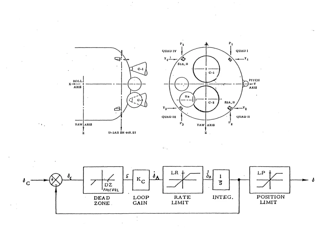
Next, cprop (Appendix F) is called. Three subroutines are called in this model: actuate (Appendix G), liqeng (Appendix H), and rcseng (Appendix I). The CENTAUR vehicle has two main engines and twelve rcs engines. Of the rcs engines, four are settling engines, four are pitch engines, and four are yaw engines. Please see figure 2 for a schematic of the location of these engines. Every time it is called, cprop loops fourteen times, once for each engine.

During the first two loops, first actuate is called. This model computes deflections of the CENTAUR main engine nozzles during burns as a function of the Powered Autopilot Software commanded deflections. These

commands, which are piped every 20 milliseconds of simulation time, are EOP, EOQ, and EOR. They can be found in table 2. The subroutine actuate

takes these commands, and through a feedback loop, compares them versus current angle states to obtain a correction value. This correction value is then filtered through a dead zone to assure the correction is large enough to

necessitate implementation. Afterwards, a loop gain constant is applied, followed by a rate limit to prevent deflection changes from happening too quickly. An integrator is then used, as well as final angle limits on engine deflections. A schematic of the actuator feedback loop can be found in figure

3. Actuate then returns a primary (pitch) deflection and a secondary

(yaw/roll) deflection for each engine.

The liqeng subroutine is then called, which computes a thrust vector and weight flow rate for each main engine. The thrust direction is

determined using the engine deflections calculated by actuate. Both the thrust magnitude and the weight flow are determined through interpolation using a variable representing the time the engine has been turned on. The reason for this is that the main engines have a start-up period which takes about three seconds before nominal full thrust is achieved. Similarly, once the propellant valves are closed at the end of a burn, there is a tail-off period for which this interpolation is also used. Once these values are calculated, they are returned to cprop which then sums up the resulting forces and moments about the body. The moments are easily determined since the location of each engine relative to a point referred to as station zero is known, as well as the center of gravity relation to station zero which was determined in cmass .

During loops three through fourteen of cprop , the rcseng is called. This subroutine makes use of the scusw(6,16) variable piped from the software. This variable is further discussed in the ADA software section of this paper. None-the-less, the scusw(6,16) contains six arrays of sixteen logical values representing discrete commands from the software. Among these commands are requests to either thrust or not thrust any of the twelve RCS

X- 4

X-- -

-AXIS

ID-IAI SN 440.57

ENGINE CONFIGURATION AND NONLINEAR ACTUATOR MODEL

I3I'T'CII A-y AXIS

6_C

engines. Reasons for using these engines could range from settling the propellant, to performing thermal rolls during coast phases, to orienting the vehicle in the appropriate position prior to a burn, to etc.... The rcseng subroutine checks which RCS engines are commanded on, and returns a value for the engine thrust vector and Hydrazine propellant flow rate per engine. No interpolations of start-up's or tail-off's are needed, since such fluctuations for RCS engines are minor and therefore negligible. Once the RCS engine thrust vector is computed in the engine frame, it is then

transformed to body coordinates using a predefined engine configuration model. The thrust magnitude and direction, and the weight flow are returned to cprop , which then sums up the resulting forces and moments about the body to those calculated for the main engines.

The following routine called is wtflow (Appendix

J),

which computes the total weight flow for each tank (main propellant and hydrazine), as well as the total weight flow overboard for the vehicle. This is done using the individual engine weight flows calculated in both liqeng and rcseng , and adding them up to calculate the flow rate of each;tank. These flow rates are integrated through the RK2 or RK4 method offered within the proconsul simulation, and new values for tank weights are therefore available in the next cycle for the routine cmass , which, as mentioned earlier, needs those values to calculate total vehicle weight.

Next, newton (Appendix K) is called to calculate sensed and inertial accelerations. The thrust forces calculated by cprop are used to determine a sensed acceleration in the body frame. This value is essential for the software navigational module and is therefore calculated to be piped to the software. More on the feedback required by the software from the dynamic side can be found in the next section of this report. Next, a true acceleration is computed in the inertial frame using the thrust forces as well as gravity. This

acceleration is then integrated, just as the weight flow rates were, in order to obtain both velocity and position values needed by the georel routine on the next cycle.

Finally, euler (Appendix L) is called. This model computes the three-degree-of-freedom rotational equations of motion. It computes angular

acceleration from Euler's rotational dynamics equation. It also computes the attitude quaternion rate from the quaternion analog of Poisson's rotational kinematic equation. These quantities are integrated to obtain the rotational state, consisting of the attitude quaternions and the angular velocity. The quaternions are needed by both the dynamics and the software.

2.2 Software

At the beginning of every 20 millisecond cycle, parameters required by the software are piped from the dynamic side, at which time one loop of the software is run. The software is written in ADA, and is a copy of the package used on the real on-board CENTAUR computer. This package is composed of many modules: the antenna select, attitude error, coast auto-pilot, coast guidance, discrete priority, hydrazine monitor, minimum residual shutdown, navigation, powered auto-pilot, powered guidance, post injection, sequencer, steering interface, cvaps, propellant utilization, and operating system. In order for the software to operate in conjunction with the dynamic side of the simulation, some adaptations had to be performed.

First, the operating system has a lot of machine language associated with it. This module serves to both run the rest of the modules and as a link

to the physical sensors of the vehicle. Therefore, most of this module needed to be eliminated and replaced by both a top level software routine and the

ADA side of the pipes, which read in the physical information that would

have otherwise been received from the sensors. The top level routine will be described in detail. However, little will be said about the dozens of alterations done to operating system routines that were not eliminated. Without in-depth knowledge of the software package as a whole, such detail will not aid the reader with a better overview understanding and only confuse the issue.

Second, both the cvaps and the propellant utilization modules are not being used. The cvaps has been removed since it requires many sensor

inputs that are not available through the existing dynamic models. However, only the cvaps ' requests for settling affect the mission's trajectory, and these have been taken into account. The propellant utilization has been left intact, but has been stubbed out. In other words, the top level software routine

simply does not call this latter module. The propellant utilization can affect the mission's trajectory by changing the mixture of the fuel and oxidizer during a burn. However, the look-up tables for engine thrust that are read by the dynamic subroutine liqeng take into account the mixture fluctuations for a nominal mission.

Finally, some adaptations needed to be made for the fact that the mission modeled in this program begins at Titan IV/CENTAUR separation. In the real mission, the CENTAUR software is initialized and the system goes inertial at 62 seconds prior to liftoff. However, the simulation time during which the CENTAUR is ascending on Titan IV's shoulders is not of any use to the utility of this simulation and therefore would be a waste of simulation time. Therefore, it was decided to initialize the program only at the point of separation.

2.2.1 Software modules

The antenna select module serves to keep track of Earth based antennas such that telemetry may be sent down during coast phases of the

mission. This module calculates vectors from CENTAUR's antennas to the Earth based ones and requests attitude changes in order to send the

transmissions at appropriate times.

The attitude error module receives attitude information from the dynamic side and steering vector increments from steering interface in order to calculate CENTAUR body axis vector changes and their errors. This

information is passed on to powered auto-pilot during burn phases and to coast auto-pilot during coast phases to implement necessary changes. Please see figure 4 for a flowchart of the guidance, navigation, and control

interactions of the CENTAUR software.

The coast auto-pilot receives the attitude error information and calculates rcs engine on and off commands (See figure 4). These commands are then passed onto discrete priority (discussed later) and are later sent to the dynamic side via the scusw(6,16) variable.

,71pabC tpycasuaaa.7 & JIL,,1 March 8-10, 1

GUIDANCE NAVIGATION AND CONTROL - BLOCK

II

IMPACTS

The coast guidance receives the navigation state from navigation (discussed later) and computes steering coefficients (See figure 4). This module also retargets burns to optimize performance. For example, if the Titan IV performs better or worse than nominal, the coast guidance will retarget to attain the most desirable final orbit that is achievable.

The discrete priority module receives all discrete commands from the rest of the modules and sets priorities to be passed onto the dynamic side. For example, using already discussed modules, antenna select may request a certain attitude while coast auto-pilot requests another through commanded rcs thrusting. The discrete priority module sorts out the requests and loads the correct arrays of commands into the scusw(6,16) variable to be piped to the dynamic side.

The hydrazine monitor keeps track of the length of burns for all rcs engines and therefore computes the level of hydrazine propellant remaining. Extra hydrazine propellant is allotted for all coast phases. If this surplus is not used, then, before each burn, this module will command the settling rcs thrusters to be turned on in order to deplete the extra weight. This results in extra performance. Also, burning this excess using only the settling thrusters does not result in attitude changes since they run parallel to the roll axis of CENTAUR.

The minimum residual shutdown module monitors levels of main propellant. It these levels drop below a residual level, this module

commands main engine shutdown in order to avoid off centered thrusting. If CENTAUR runs out of propellant, one engine may shut down before the other, causing the vehicle to tumble. This undesirable situation is prevented through the implementation of this module.

The navigation module receives sensed velocity increments (sensed acceleration) from the dynamic side and computes position and velocity vectors for the software (See figure 4). This module also has its own gravity model. Therefore, since many of the calculations performed are redundant with those performed on the dynamic side, running the simulation provides

The powered auto-pilot receives attitude error information and calculates gimbal angles to be piped to the dynamic side (See figure 4). The gimbal angles are the previously discussed EOP, EOQ, and EOR variables that are fed into the dynamic subroutine actuate.

The powered guidance receives the navigation state from navigation and computes steering coefficients just as the coast guidance does (See figure 4). This module makes use of steering equations and contains the heart of CENTAUR's burn performance. It commands attitude holds during start-ups and tail-offs, and its complexity as a whole is impressive.

The post injection is also a guidance module (See figure 4). It operates after final orbit insertion (end of the third burn) and calculates guidance commands for CENTAUR/payload separation and the maneuvers performed afterwards.

The sequencer keeps track of the order of events of the mission and mission time. This module performs many necessary functions that are

mainly sequence or time dependent.

The steering interface receives steering coefficient values from guidance and transforms them into steering vector increments for attitude

error (See figure 4).

The cvaps calculates the state of the main engine fuel and oxidizer, and requests propellant settling and venting when appropriate.

The propellant utilization module calculates main engine propellant utilization and varies the mixture as appropriate if either the fuel or oxidizer levels become too low.

2.2.2 Top level software routine

The top level software routine, ADAEXECUTIVE (Appendix M), was created to run the entire software package in the simulation. This routine is called once every cycle, which corresponds to a time frame of 20 milliseconds. Although many software modules run at a frequency of 50 Hz, some are called at lower frequencies. Therefore, an index, which increases by one every cycle, was included in the executive. When this index reaches a value of 400, which corresponds to a time frame of 8 seconds, it is returned to zero. By analyzing the ADA_EXECUTIVE code, one can see that, for example, the coast

guidance module is called only when the index value equals one. This

means that the module is run every 8 seconds only.

The executive routine also calls the appropriate routines during particular phases. The sequencer module assigns values to the variable iphase, which represents the timeline position in which the vehicle currently finds itself. For example, an iphase value equal to seven represents the first burn. It was previously mentioned that the coast.iguidance runs at 8 second

intervals. However, this module also operates during coast phases only. Therefore, when iphase has a value equal to 7, the coast guidance should not be running.

Although, as was stated earlier, this paper will not go into detail on the many changes done to the operating system software module, there is one particular subroutine of interest. The OS_SET_DISCRETE_OUTPUT subroutine (Appendix N) keeps track of all the 64 discrete switches that are either on or off. This routine is fed information from the discrete priority module as to which switches are to be commanded on or off, and stores these

commands in the variable scusw(6,16) discussed earlier. Each of the sixteen memory locations in the six arrays carries a value of true or false. The

2.2.3 Cvaps and propellant utilization

The cvaps is not modeled since the inputs required from sensors for this module are too extensive. As stated earlier, the cvaps calculates the state of the main engine fuel and oxidizer, and requests propellant settling and venting when appropriate. In order to perform this task, this module needs complete information from many sensors within both the fuel and oxidizer

tanks as to the pressure, density, temperature, and state of these propellants in different areas of the tank. The dynamic models are not prepared to provide such data. Building dynamic models for such a task would easily double the size of the simulation and are not part of the required responsibilities of the Guidance Analysis Department.

Since the cvaps module is not modeled in this simulation, some work and restructuring was needed in order to maintain a vital role of this module. Depending on the conditions of the propellants, this module has the

authority to request propellant venting. However, in order to vent,

CENTAUR must first settle the fuel and oxidizer by thrusting with the rcs

engines that run parallel to the roll axis of the vehicle. Although the change in both velocity and position due to the settling is not great, it is none-the-less not negligible. Therefore, a dummy routine (Appendix O) became essential to command the settling activity. This routine commands settling twice during the transfer orbit coast, representing the two venting windows that nominally occur on a perfectly predicted mission.

As stated earlier, the propellant utilization module calculates main engine propellant utilization and varies the mixture as appropriate if either the fuel or oxidizer levels become too low. However, the dynamic side is once again not capable of provided the required inputs for this module. The dynamic models contain only two tanks. One is the rcs propellant tank, which is filled with hydrazine. The other is the main propellant tank, which represents a combination of both the fuel and oxidizer tanks. The engines burn at a predetermined nominal mixture, and the total fuel plus oxidizer flow rate, which is read off a table, is subtracted from this one tank's weight. Therefore, the propellant utilization is simply not modeled. However, since

this module does not output any values needed by other software modules, it became sufficient to simply neglect calling this package from the executive.

3.0 NLP2 OPTIMIZER

The NLP2 Optimizer Algorithm, built by John Betts and Wayne Hallman, is a general-purpose method for solving the nonlinear

programming problem. Here is an overview of the optimizer from its documentation, written by the authors of the software:

It performs two major operations. The constraint satisfaction phase, which is performed first, determines a feasible point for the nonlinear constraint functions. A generalized secant algorithm is used which computes corrections using an equality constrained least distance programming algorithm. If this technique fails to locate a feasible point, a gradient-based method is employed. If this technique also fails, the constraint error is minimized using a general unconstrained

minimization algorithm.

After a feasible point is located, the algorithm solves a series of

equality-constrained optimization problems. The equality-constrained optimization phase consists of a sequence of problems with the set of

active constraints defined by the basis determination procedure. Each equality-constrained problem is solved using an orthogonal

decomposition of the problem variable. One subset of the variables is used for eliminating the active constraints from the problem. The constraint elimination process is achieved using a generalized secant method with a trust region strategy. The other subset of variables is adjusted to minimize the objective function restricted to the surface of the active constraints. The unconstrained minimization technique employed is selected by the user from a finite difference Newton

method, a quasi-Newton method using recursive Hessian updates, and a robust least squares option. These techniques use an inequality-constrained univariate search technique to adjust the step length. If a previously satisfied inequality constraint is encountered during the minimization process, the iterations are terminated and the offending constraint is added to the active set. Otherwise, minimization proceeds to the optimum point, at which time deletions from the active set are

considered. When no additions or deletions are made from the active set, the algorithm terminates at the local solution.

Among the many inputs to the NLP2 program are XBAR, CBAR, and FBAR. XBAR represent the parameters that NLP2 can change in order to optimize the simulation. CBAR represent the constraints. Finally, FBAR represents the objective function which in this case is fuel consumption. By using different XBAR values, NLP2 works to minimize FBAR while meeting CBAR restrictions.

The NLP2 optimizer was integrated into the proconsul simulation by dividing its major functions into events. These events occur either at the beginning or the end of the simulation. Proconsul gives the user the ability for an event to monitor the trigger for any other event. In other words, it does not matter the physical order of events within the code, but rather what triggers are monitored by the current event. At the same time, the only way to trigger another event, is to have the trigger conditions become true. In a flight simulation, since events are based on a timeline, all events simply monitor the next one's trigger. For example, the first pre-burn event

monitors the first main engine burn trigger, and so on. In the integration of the optimizer to the flight simulation, the order of which event follows which becomes more complex. As can be seen in figure 5, some NLP2 events branch out into more than one other. In this case, whichever trigger

condition is satisfied first will determine which event becomeis the next one. Also, there occurs some loops back to previously called events. However, due to the flexibility of Proconsul, this complication did not become a barrier, and therefore the appropriate sequence of events was achieved.

In running the targeting program, first the optimization algorithm is called. From there, either evaluate function or the jacobian algorithm is called. Evaluate function calls for a complete run of the flight simulation from beginning to end. After the run, constraint check is called to calculate if the constraints were met. From there, the jacobian algorithm prepares a Jacobian matrix for optimization purposes. Afterwards, either evaluate function is called again, or output is called. Output serves to simply give

NLP2

Flow Chart

Guidance Analysis Department

Figure 5

THE AEROSPACE CORP OR ATION

constraints are met and the objective function is optimized, the objective function solved event is called to output final results, and the run is ended. Please see figure 5.

4.0 TARGETING PROGRAM

The purpose of this project was to build a targeting program that could handle large, 6-DOF simulations (i.e., uses moments and body rotational kinematics). Traditionally, targeting programs have only been 3-DOF (i.e., simple point mass and thrust vector), due to the enormous time

consumption of optimizing a more sophisticated flight simulation. The 3-DOF optimized trajectory would then tweaked be to obtain a closer solution to

the real answer. In order to target a 6-DOF simulation directly, a fast-running targeting program must be built.

The specific targeting program built was used to optimize the

CENTAUR 6-DOF TC-17 mission for second and third burn fuel consumption

minimization. This optimization is constrained to meet the final orbit desired at the end of the third burn. In terms of NLP2 variables, the fuel consumption would translate into FBAR, the variable to be minimized. Also, since five variables are needed to define an.brbit, the values of these five variables for the final orbit desired would translate into CBAR. In

actuality, the final orbit for this mission is not circular. The apogee always occurs at the location of the third burn. Therefore, since this parameter is already defined, there are only four constraints that are translated into CBAR.

Traditionally, such targeting programs have used burn variables as the parameters XBAR to be varied by the optimizer. In an impulsive burn

targeting program, such variables would include a AV, and two angles

determining pitch and yaw from the velocity vector. In the case of the TC-17 mission, such a simplified simulation would then include only three

parameters per burn plus a time of coast variable. Since this amounts to only seven XBAR parameters and there are four CBAR constraints, the optimized solution to the problem can be solved using a relatively small number of flight simulation runs.

However, an impulsive simulation is a poor model for the finite burn situation found in real life. In using a finite burn simulation, even a 3-DOF one, the number of XBAR parameters needed to be yaried by the optimizer

increases substantially. These parameters would now include time of burn, angular velocity of the thrust vector during the burn, and many other complicating factors. In addition, many such variables may be subject to physical or software constraints. For example, the angular velocity of the

thrust vector may be limited by the maximum gimbal angle of CENTAUR's main engine nozzles. This would be a physical limitation. Also, the angular

velocity of the thrust vector would be forced to remain zero during the initial stages of a burn for tumbling avoidance reasons. This would be a software limitation.

Therefore, there are two problems. First, with all these added variables, the number of XBAR parameters versus CBAR constraints increases

substantially, forcing the optimizer to run the flight simulation many more times to solve the problem. If the run involved is a full-up 6 DOF simulation whose running time is up to 3 hours, as the one that is used with Proconsul described earlier, having to run it hundreds if not thousands of times to solve the optimization problem becomes time prohibitive. Also, the limitations that need to be taken into account with all these new variables becomes a coding nightmare.

The approach in this targeting program was to use the transfer orbit parameters as the XBAR variables in conjunction with the guidance software. Since there are only five variables that define the transfer orbit as well, the optimization problem becomes simplified. Also, there are no limitations on the values of these variables. CENTAUR's guidance is trained to tailor the burns as necessary to match the next desired orbit. As the optimizer fiddles with the transfer orbit variables, the second burn will automatically be adjusted such that CENTAUR will end up with the desired transfer orbit. Also, since the final orbit parameters are constraints that are hard coded into the software, the guidance will force CENTAUR to adjust its third burn as well in order to meet the final orbit parameters from a now different than nominal transfer orbit. Therefore, by simply using the transfer orbit variables for XBAR, both burns two and three are automatically adjusted. This being the case, optimizing on the most fuel efficient transfer orbit becomes

Please see figure 6 for a picture of the transfer orbit, as well as the surrounding second and third burns.

There are many advantages to this approach. Since there are only five XBAR variables and four CBAR ones, the optimizer problem is solved

relatively quickly. Although the speed at which this problem is solved is a function of how close the initial inputs are to the optimized answer, with the inputs used in this targeting program the solution was found with only 26 runs of the flight simulation. Since the targeting program is so fast-running due to this new approach, it is acceptable to use the full-up 6 DOF flight simulation described earlier in this paper. By using this simulation which

contains almost all the real on-board computer software modules and is dynamically modeled in 6 degrees-of-freedom, the answer obtained is very accurate. All aspects of the mission are taken into account, from the many settling phases, to the main engine burn start-ups and tail-offs, to every rcs thrusting that has the most remote impact on the mission trajectory. Also, since almost all the software modules are used and the dynamic modeling is extensive, the optimized targeted trajectory is gua.ranteed to be custom fitted to the CENTAUR mission. Therefore, there is no doubt that the CENTAUR can and will fly the optimized trajectory.

It is important to point out that there is a limitation to this targeting program. By using the transfer orbit parameters as the XBAR variables, the CENTAUR software becomes an integral component of the targeting

program, since it alone can modify the burns surrounding the transfer orbit. Therefore, the optimized solution is subject to any imperfections that may accompany the steering equations and all other aspects of the CENTAUR software. It is conceivable that a lower fuel consumption trajectory that operates between park orbit and final orbit could exist. However, such a trajectory would be beyond CENTAUR's ability to fly it.

CENTAUR Trajectory

Burn 3

Guidance Analysis Department

Figure 6

* THE AEROSPACE

5.0 RESULTS & SUGGESTIONS FOR FUTURE

RESEARCH

In order to properly evaluate the targeting program, two topics need to be addressed. First, an estimate of the efficiency of the targeting program needs to be included. In other words, how fast is the simulation optimized? Second, an estimate of the accuracy of the optimized trajectory needs to be included.

As mentioned before, using the transfer orbit elements as inputs to the optimizer allowed the simulation to be targeted in only 26 runs. In 3-DOF targeting programs for CENTAUR missions, optimizing takes hundreds of simulation runs. However, this comparison is misleading. The speed at which a simulation is optimized is a function of the accuracy of the initial inputs. These initial inputs were obtained by first using a 3-DOF, impulsive burn simulation. and optimizing it. This is the same process that is used in a 3-DOF, finite burn targeting program. However, as expected, the first attempts to optimize using the 6-DOF, finite burn targeting program met with various problems. As the debugging process took place, the initial inputs were

simultaneously improved. Therefore, if a new mission were to be targeted using the 6-DOF, finite burn program, it is unlikely that the initial estimates would be so accurate as to allow optimization to occur in only 26 runs of the flight simulation. In an educated guess, fifty to seventy-five runs would have been necessary had the targeting program used the initial inputs first found from the 3-DOF, impulsive burn targeting method.

The contractor is solely in charge of targeting CENTAUR missions. This task has always been performed using a 3-DOF, finite burn targeting program, the results being then tweaked to account for moments and body rotational kinematics. A comparison between the contractor's and the 6-DOF, finite burn targeting program's transfer orbits and final orbits can be found on the next page.

Contractor Targeting 6-DOF Finite Burn Targeting Orbit Elements Transfer Orbit Final Orbit Transfer Orbit Final Orbit Apogee (ft.) 138,832,317 138,998,568 138,841,858 139,014,112 Perigee (ft.) 20,712,835 128,787,697 20,713,349 128,792,800 Inclination (deg.) 24.8265 5.0134 24.8265 5.0134 Arg. of Perigee (deg.) 178.254 169.782 178.254 169.778

RAAN (deg.) 312.978 310.368 312.979 310.366

From the comparison above, it becomes clear that both methods validate each other by producing similar results. Therefore, if nothing else, the 6-DOF, finite burn targeting program can be used as a verification tool as the many used by the Aerospace Corporation in its on-going work to validate the contractor's methods and results for the United States Air Force.

Although the original goals set out have been accomplished by building a working 6-DOF, finite burn targeting simulation, there is much work that remains to be done that can solidify the process. First, it would be useful to make a full comparison of the targeting program to traditional methods, specifically concentrating on the efficiency of the 6-DOF approach. Next, the flight simulation used should be simplified to increase the

efficiency of the targeting program. There are many software function that are not essential in obtaining the fuel consumption minimized trajectory and could, therefore, be removed. This would decrease the running time of the flight simulation, and, in turn, result in a faster running targeting program. Also, the testing of the 6-DOF approach should be expanded to include other CENTAUR missions, and, preferably, other vehicles all together. This would verify the usefulness, or lack thereof, of the targeting program, as well as provide a larger test bed for the method. Finally, it might prove beneficial to test other optimizer algorithms to determine the best one available for a 6-DOF targeting method.

-Sgeorel.f =====

subroutine georel

**********************************************************************

k purpose: earth-relative frames and positions *

* This model is used at the beginning of each derivative pass to

* compute basic position quantities used by other models. In

* addition, it constructs the LH and GLH frames for the vehicle,

* normalizes the attitude quaternion, and constructs the BODY to

* ECI DCM from the normalized quaternion.

*

* inputs:

* qb2e - Vehicle attitude quaternion

* (Coordinate rotation quaternion,

* BODY to ECI)

*

* outputs:

* xymag - Planar position magnitude (ft)

* posmag - Position vector magnitude (ft)

* gclat - Geocentric latitude (rad)

* sgclat - Sine of geocentric latitude

* cgclat - Cosine of geocentric latitude

* gdlat - Geodetic latitude (rad)

* sgdlat - Sine of geodetic latitude

* cgdlat - Cosine of geodetic latitude

* geodalt - Geodetic altitude (ft)

* qb2e - Vehicle attitude quaternion (normalized)

* tb2e - Coordinate rotation DCM, BODY to ECI

* tglh2e - Coordinate rotation ICM, GLH to ECI

tlh2e - Coordinate rotation DCM, LH to ECI

* * subprograms: * subroutine geocent * subroutine geodet * subroutine makh2e * subroutine qnormald * subroutine q2dcmd * * commons: * eulout (qb2e)

* geoout (all other outputs)

*

* author: L. Andrew Campbell

*

* date:

* first coded: 01-Feb-19/91

* last modified: 26-Mar-19/91

* 7/11/93 changed common names TLM

* 1/22/94 changed qnormal and q2dcm to qnormald and

* q2dcmd TLM

* 8/15/94 deleted makg2e for CENTAUR simulation (A. Thomas)

* ********************************************************************** ! commons include 'eulout.cmn' include 'geoout.cmn' call geocent call geodet call makh2e

call q2dcmd (qb2e, tb2e) return

geocent.f===

subroutine geocent

* purpose: compute geocentric variables

* This model is called by GEOREL to compute the basic geocentric

* variables from the vehicle position.

inputs: * outputs: * * * * * * * * * commons: * * * I. * * xeci dxeci omege time lguidcn mi2e xymag posmag velmag sgclat cgclat gclat long

Vehicle position vector [ECI] (ft) Vehicle velocity vector [ECI] (ft/sec)

Earth angular speed (rad/sec) Current simulation time (sec)

L guidance constants from flight software Transformation matrix, uvw to tod eci

Planar Position Magnitude (ft) Position Vector Magnitude (ft) Velocity Vector Magnitude (ft/sec)

Sine of geocentric latitude Cosine of geocentric latitude Geocentric latitude (rad)

Longitude of the vehicle (rad)

nwtout (xeci, dxeci) grvinp (omege)

timing (time) lguidcn (lguidcn)

uvw (mi2e)

geoout (cgclat, gcla t, posmag, sgclat, xymag, velmag, long)

* author: L. Andrew Campbell

* date:

* first coded: 01-Feb-19/91

* last modified: 26-Mar-19/91

* 7/11/93 changed common names TLM

* 1/22/94 made real local tmp type double TLM

* 9/2/94 added "velmag" calculation for CENTAUR (A. Thomas)

* 9/9/94 added "long" calculation for CENTAUR (A. Thomas)

* ! constants include kearth.par include ktimes.par ! locals double precision + tmp,

+ tmpang, I angle between vehicle & launch site at go-inertial

+ rotang, I angle of Earth's rotation since go-inertial

+ tmpvl(3), ! lguidcn(7:9) crossed with lguidcn(1:3)

+ tmpv2(3), ! mi2e crossed with tmpvl

+ cgrnang, ! cos of angle between launch site and greenwich

+ grnang ! angle between launch site and greenwich

! commons

include 'geoout.cmn' include 'nwtout.cmn'

include 'grvinp.cmn' include 'timing.cmn'

include 'lguidcn.cmn' include 'uvw.cmn' xeci(1)**2 + xeci(2)**2 sqrt(tmp) tmp +- xeci(3)**2 sqrt(tmp)

dxeci(1)**2 + dxeci(2)**2 + dxeci(3)**2

sqrt(tmp)

xeci (3)/posmag xymag/posmag

asin(sgclat) ! between +/- pi/2 tmpang = atan(xeci(2)/xeci(1))

rotang = omege * (time + 62.0do0) call vcrossd(Iguidcn(7:9)

call mv3multd(mi2e,tmpvl, cgrnnng = tmpv2(1)

grnng - acos(cgrnang)

long = tmpang - rotang

,iguidcn(1:3),tmpvl) tmpv2) - grnang tmp xymag tmp posmaqg iwp velm-g sgClat cgclat gclat return end

Sgeodet.f =====

subroutine geodet

* purpose: compute geodetic variables from geocentric

* This model computes the geodetic altitude and the angle between

* geocentric and geodetic vertical. To do this it uses geocentric

* latitude and earth shape parameters. The algorithm used is

* described in: *

* Cretcher, C. K. Geodetic/Geocentric Conversions.

* Report ATM-69(4112-50)-24. The Aerospace Corp.

*

* inputs:

* eesq - Earth ellipticity squared * eqtrad - Earth equatorial radius (ft) * posmag - Position vector magnitude (ft) * gclat - Geocentric latitude (rad)

* sgclat - Sine of the geocentric latitude * cgclat - Cosine of the geocentric latitude * outputs:

* gdlat - Geodetic latitude (rad) * geodalt - Geodetic altitude (ft)

* sgdlat - Sine of the geodetic latitude * cgdlat - Cosine of the geodetic latitude *

* Note: the local variable lambda is the angle between

the verticals mentioned in the purpose section

* commons:

* grvinp (eesq, eqtrad)

* geoout (gclat, posmag, sgclat, cgclat, all outputs)

* author: L. Andrew Campbell

*

* date:

* first coded: 01-Feb-1991

* last modified: 26-Mar-1991

* 7/11/93 changed common names TLM

* 1/22/94 made real literals and locals type double TLM

*

! constants

include 'kearth.par'

! locals

integer iter

double precision dstar, eps, x, y, d, lambda

! commons

include 'geoout.cmn' include 'grvinp.cmn'

dstar = sqrt(l.0dO - eesq * cgclat * cgclat) x = sgclat * cgclat * eesq * eqtrad / dstar y = eqtrad * dstar

eps = 0.OdO sgdlat = sgclat

do iter = 1, 3

d = sqrt(1. OdO - eesq * sgdlat * sgdlat)

geodalt = (posmag / sqrt(1.OdO + eps * eps)) - d * eqtrad eps = x / (y + geodalt * d / dstar)

lambda = atan(eps) gdlat = gclat + lambda

sgdlat = sin(gdlat)

enddo

cgdlat = cos(gdlat) returni

gravity.f =====

subroutine gravity

! locals

integer i

double precision unitr(3), unitnp(3), ni, n2, cosg, gr, gnp double precision guvw(3)

! commons

include 'grvout.cmn' ! (geci)

include 'geoout.cmn' ! (posmag)

include 'lguidcn.cmn' ! (lguidcn)

include 'nwtout.cmn' ! (xeci)

include 'uvw.cmn' _{! (rcn, me2i, mi2e)}

call mv3multd(me2i,xeci,rcn) unitr(1) = rcn(1)/posmag unitr(2) = rcn(2)/posmag unitr(3) = rcn(3)/posmag unitnp(1) = lguidcn(1) unitnp(2) = lguidcn(2) unitnp(3) = lguidcn(3) cosg = unitr(1)*unitnp(1)+unitr(2)*unitnp(2)+ & unitr(3)*unitnp(3) nl = 1.4076458d16 n2 = 2.0019662d28 gr = -nl/posmag**2 + (n2/posmag**4)*((5*cosg**2-1)/2) gnp = n2*cosg/posmag**4 do i = 1,3

guvw(i) = gr*unitr(i) - gnp*unitnp(i)

enddo

call mv3multd(mi2e,guvw,geci)

return end

cmass.f

subroutine cmass

S purpose: CENTAUR total weight & mass, tabular cg and inertia

* This model computes a total vehicle weight as the sum of * the static weight (structure), payload weight, and tank

* weights (RCS and main engine propellants). The vehicle

* center of gravity location and inertia are then determined

* by table lookup on weight.

* inputs: wstatic wpayld tankwt(.) jetwt cgrtfp(.) ixxtfp iyytfp izztfp pxytfp pxztfp pyztfp cgrlob(.) ixxlob iyylob izzlob pxylob pxzlob pyzlob outputs: vehwt vmass vehcg(3) vint(3,3) cgrlob(.) ixxlob iyylob izzlob pxylob pxzlob pyzlob - Static weight (lb) - Payload weight (lb)

- Tank . total weight (lb)

- Jettison weight (lb)

- cg tabular function pointers

- x moment of inertia tabular function pointer - y moment of inertia tabular function pointer - z moment of inertia tabular function pointer - xy prod. of inertia tabular function pointer - xz prod. of inertia tabular function pointer - yz prod. of inertia tabular function pointer - ptrs to cg previous lower bounding breakpoints - pointer to x moment of inertia previous

lower bounding breakpoint

- pointer to y moment of inertia previous

lower bounding breakpoint

- pointer to z moment of.:inertia previous

lower bounding breakpoint

- pointer to xy prod. of inertia previous lower bounding breakpoint

- pointer to xz prod. of inertia previous lower bounding breakpoint

- pointer to yz prod. of inertia previous lower bounding breakpoint

- Total vehicle weight (lb)

- Total vehicle mass (slug) - Vehicle cg location [BODY] ft

- Vehicle inertia tensor, cg-centered

[BODY] (slug-ft**2)

- ptrs to cg current lower bounding breakpoints - pointer to x moment of inertia current

lower bounding breakpoints

- pointer to y moment of inertia current

lower bounding breakpoint

- pointer to z moment of inertia current

lower bounding breakpoint

- pointer to xy prod. of inertia current lower bounding breakpoint

- pointer to xz prod. of inertia current lower bounding breakpoint

- pointer to yz prod. of inertia current lower bounding breakpoint

* subprograms:

* commons:

double precision function dlindl

masbepo (wstatic, wpayld, jetwt)

mastfp (cgrlob, cgrtfp, ixxlob, ixxtfp, iyylob, iyytfp, izzlob, izztfp, pxylob, pxytfp, pxzlob, pxztf.D,

* pyzlob, pyztfp)

* masout (vehcg, vehwt, vint, vmass)

* wtfout (tankwt)

* author: L. Andrew Campbell

*

* date:

* first coded: 01/01/91

* last modified: 26-Mar-91

* 7/8/93 modified to use new interpolation function

rlinrl() T.L. Morgan

* 7/10/93 changed common and variable names TLM

* 7/17/93 replaced variable ceslm2w with GSLM2W parameter TLM

* 1/21/94 changed knumbr.par to ksetrm.par and function

* rlinrl() to dlindl() TLM

* 8/26/94 Modified for Centaur. S.T. Dunham, A.P. Thomas

! constants include 'kintrp.par' include 'ksetrm.par' include 'kphysc.par' ! locals integer i ! commons include 'masbepo.cmn' include 'mastfp.cmn' include 'masout.cmn' include 'wtfout.cmn' ! externals

double precision dlindl ! double linear interpolation in a

external dlindl ! double univariate table

******** **** *** ************************************************* * **

! subtract vented wt. from main tank wt.

tankwt(1) = tankwt(1) - jetwt jetwt = 0.d0O

! add tank weights to static wt & pyload wt to get total

vehwt = wstatic + wpayld + tankwt(1) + tankwt(2)

vmass = vehwt / GSLM2W

! interpolate for center of gravity

do i = 1,3

vehcg(i) = dlindl (cgrtfp(i), vehwt, cgrlob(i), EXTEND) enddo

I interpolate for components of inertia tensor

vint(l,1) = dlindi (ixxtfp, vehwt, ixxlob, EXTEND)

vint(2,2) = dlindl (iyytfp, vehwt, iyylob, EXTEND)

vint(3,3) = dlindl (izztfp, vehwt, izzlob, EXTEND)

vint(2,3) = dlindl (pyztfp, vehwt, pyzlob, EXTEND)

vint(l,3) = dlindl (pxztfp, vehwt, pxzlob, EXTEND) vint(1,2). = dlindl (pxytfp, vehwt, pxylob, EXTEND)

vint (3,2) vint (3, 1) vint (2,1) = vint (2,3) = vint (1, 3) = vint (1, 2) return end

subroutine cprop

purpose: CENTAUR propulsive forces and moments

* This model calls a liquid main engine model, and an RCS engine

* model. The resulting forces are summed and the moments about

* both the BODY frame and cg are computed.

*

* inputs:

* engset - ENDSET terminated set of active engines

* engtap - engtap(*,n) is the thrust application

* point [BODY] (ft) for engine n

* vehcg - vehicle center of gravity [BODY] (ft)

* flowflg - flag determining whether main engine thrust

* and weight flow tables are active

*

* outputs:

* engf - engf(*,n) is engine n thrust [BODY] (lb)

* engwdt - engwdt(*,n) = weight flow (lb/sec)

* fpbody - propulsive force [BODY] (lb)

* mpbody - prop. moment about body [BODY] (ft-lb)

* mpcg - prop. moment about cg [BODY] (ft-lb)

* * subprograms: * subroutine actuate * subroutine liqeng * subroutine rcseng * subroutine vcrossd * commons: * engbepo (flowflg) * enginp (engtap) * masout (vehcg)

* prpout (engf, engwdt, fpbody, mpbody, mpcg)

*

* author: L. Andrew Campbell

*

* date:

* first coded: 01/01/91

* 7/9/93 reorganized commons and changed names T.L. Morgan

* 10/14/93 added test for call to SRMU actuator model RJH

* 1/21/94 changed knumbr.par to ksetrm.par, routine vcross

* to vcrossd, and made real literals and local

* variables type double TLM

* 2/2/94 merged double precision and SRMU versions, made

* names of local variables more meaningful, changed

* variable name mphat(.) to mpbody(.) TLM

* 8/12/94 converted to CENTAUR simulation by A. Thomas

*

*********************************************************************** *

! constants include 'ksetrm.par'

! locals

double precision mpeng(3) ! single-engine moment about BODY

! frame [BODY] (ft-lb)

double precision mpdisp(3) ! negative of "displacement" moment

! about cg [BODY] (ft-lb)

integer engine ! engine number

! commons

include 'engbepo.cmn'