HAL Id: hal-02500975
https://hal.archives-ouvertes.fr/hal-02500975
Submitted on 24 Nov 2020HAL is a multi-disciplinary open access archive for the deposit and dissemination of sci-entific research documents, whether they are pub-lished or not. The documents may come from teaching and research institutions in France or abroad, or from public or private research centers.
L’archive ouverte pluridisciplinaire HAL, est destinée au dépôt et à la diffusion de documents scientifiques de niveau recherche, publiés ou non, émanant des établissements d’enseignement et de recherche français ou étrangers, des laboratoires publics ou privés.
Dynamic modeling and simulation of a concentrating
solar power plant integrated with a thermochemical
energy storage system
Ugo Pelay, Lingai Luo, Yilin Fan, Driss Stitou
To cite this version:
Ugo Pelay, Lingai Luo, Yilin Fan, Driss Stitou. Dynamic modeling and simulation of a concentrating solar power plant integrated with a thermochemical energy storage system. Journal of Energy Storage, Elsevier, 2020, 28, pp.101164. �10.1016/j.est.2019.101164�. �hal-02500975�
Dynamic Modeling and Simulation of a Concentrating Solar Power Plant Integrated
1with a Thermochemical Energy Storage System
23
Ugo PELAYa, Lingai LUOa,*, Yilin FANa, Driss STITOUb 4
5
a Université de Nantes, CNRS, Laboratoire de thermique et énergie de Nantes, LTeN, UMR6607, F-6
44000 Nantes, France 7
b Laboratoire PROcédés, Matériaux et Energie Solaire (PROMES), CNRS UPR 8521, Tecnosud, 8
Rambla de la Thermodynamique, 66100 Perpignan, France 9 10 11
Abstract:
12 13This paper presents the dynamic modeling & simulation of a concentrating solar power (CSP) 14
plant integrated with a thermochemical energy storage (TCES) system. The TCES material used is 15
calcium hydroxide and the power cycle studied is a Rankine cycle driven by the CSP. Firstly, 16
dynamics models of components written in Modelica language have been selected, developed, 17
parametrized, connected and regulated to create the CSP plant with different TCES integration 18
concepts. Then simulations were then performed to determine and compare the energy efficiency, 19
water consumption and energy production/consumption of three integrations concepts for two 20
typical days (summer and winter) and for a basic continuous production mode. After that, a 21
feasibility study has been performed to test a peak production scenario of the CSP plant. 22
23
The results showed that a TCES integration could increase the overall efficiency of the CSP 24
plant efficiency by more than 10%. The Turbine integration concept has the best global efficiency 25
(31.39% for summer; 31.96% for winter). The global electricity consumption of a CSP plant with 26
TCES represents about 12% of its total energy production for a summer day and 3% for a winter 27
day. An increased nominal power by a factor of 10 could be reached for the peak production mode 28
within one hour using the Turbine integration concept, but with a lower global efficiency (17.89%). 29
30 31
Keywords: Thermal energy storage (TES); Thermochemical energy storage (TCES); Concentrating 32
solar power (CSP); Dynamic modeling; Production mode; Integration concept 33
34
Abbreviations 35
CSP: Concentrated solar power; DNI: Direct normal irradiance; HTF: Heat transfer fluid; Int.
36
concept: Integration concept; MENA: Middle East and North Africa; PID: Proportional integral
37
derivative; SPT: Solar power tower; TCES: Thermochemical energy storage; TES: Thermal energy
38
storage
39 40
Declarations of interest: none
41
1. Introduction
42 43
Concentrating solar power (CSP) is expected to play a key role in the future energy transition 44
scenarios towards a more electrified world with low-carbon technologies [IEA, 2018]. Meanwhile, 45
thermal energy storage (TES) systems become indispensable to increase the dispachability and the 46
economic competitiveness of modern large-scale powerful CSP plants [Alva, 2018; Kuravi, 2013]. 47
Currently more than 80% of the CSP plants under construction or planned incorporate TES systems 48
[NREL, 2018; IRENA, 2018].
49 50
Sensible storage using molten salt is the most developed and commonly used TES 51
technology for existing CSP plants because of its simplicity, reliability and cost-effectiveness [Pelay,
52
2017a; b]. However, the salt corrosiveness [Ding, 2019; Walczak 2018; Wang, 2019], the limited
53
working temperature [Gimenez, 2015; Villada, 2018] and the risk of salt solidification [Vignarooban,
54
2015; Villada, 2019] are the major drawbacks remaining to be solved. Other sensible TES systems
55
have then been proposed and studied during the last years, as summarized in recent review papers 56
[Mohan, 2019; Nunes, 2019]. As an alternative, latent heat storage using phase change materials
57
(PCMs) is under intensive investigation, owing to their high density and almost constant phase 58
change temperature during charging or discharging [Lin, 2018; Nazir, 2019]. Special attention has 59
been focused on the improvement of their limited thermal conductivity through encapsulation as 60
well as nanomaterials additives [Qureshi, 2018; Tao, 2018]. 61
62
Another trend on the TES systems for CSP plants is the development of thermochemical 63
energy storage (TCES) technology based on reversible endothermic/exothermic chemical reactions 64
involving a large amount of reaction heat. TCES systems become a very attractive option because 65
of their high energy density (up to 10 times greater than latent storage) and the long storage 66
duration at ambient temperature [Prieto, 2016]. Latest advances on the thermochemical materials, 67
reactors and processes are reviewed and summarized in Refs [Liu, 2018; Jarimi, 2019]. Recently, 68
great efforts have also been devoted to investigate the appropriate coupling of the TCES system 69
with the power generating cycle (e.g., Rankine cycle; Brayton cycle, etc.) of the CSP plant [e.g.,
70
Alovisio, 2017; Cabeza, 2017; Ortiz, 2017; 2018; 2019; Schmidt, 2017; Pelay, 2019]. This process
71
integration issue plays actually a key role on the adaptation of the TCES technology to the future 72
CSP plants. Particularly in our previous study [Pelay, 2019], three TCES integration concepts using 73
Ca(OH)2/CaO couple have been proposed. Energy and exergy analyses results indicated that 74
compared to a reference plant without storage, the TCES integration could significantly improve 75
the adaptability and dispatchability of the CSP plants with the increased power production [Pelay,
76
2019].
77 78
While most of the earlier studies reported in the literature are focused on conceptual or static 79
analysis, detailed exploration of the TCES process integration issue is still lacking. The dynamic 80
behaviors of CSP plant with TCES integration are of particular importance because this type of 81
installation is inherently subjected to transient boundary conditions such as the varying solar 82
irradiation. Moreover, the dynamic simulations also make it possible to highlight the influences of 83
thermal inertia, which has usually been neglected in the static analysis but plays an important role 84
regarding the real operations of the CSP plant. 85
86
As the following work of our previous study [Pelay, 2019], this paper makes a step forward 87
by presenting the dynamic modeling & simulation of a CSP plant integrated with a TCES system 88
under real conditions. Dynamic models of each component written in the Modelica language have 89
been either adopted from the Dymola library or developed in-house. These models have then been 90
parametrized and further interconnected to build the global model for the CSP plant with TCES 91
integration. The main objectives of this study include: (1) to characterize, for the first time, the
92
dynamic behaviors of a CSP plant coupled with a TCES unit; (2) to compare the performances of 93
different TCES integration concepts under realistic variable environmental conditions; (3) to 94
showcase the feasibility of the basic continuous production mode and the peak production mode by 95
implementing advanced control strategies. The contributions of this paper are important because it 96
will expand the limited literature and provide additional insights on the dynamic behaviors of CSP 97
plants with TCES integration. The results obtained may be used for the large deployment of the 98
TCES technology in CSP plants. 99
100
The rest of the paper is organized as follows. Section 2 introduces the methodology used for 101
this study, including the proposed TCES integration concepts, the mathematic model for individual 102
component, the operation mode, the control and the initialization parameters. Section 3 presents 103
and compares the dynamic simulation results for the CSP with different TCES integration concepts 104
under the continuous production mode. Section 4 reports a feasibility study on the peak production 105
mode with the Turbine integration concept. Finally, main findings are summarized in section 5. 106 107 108
2. Methodology
109 110In this section, the three TCES integration concepts previously proposed are briefly 111
introduced. Then the dynamic model for each individual component used in the simulation is 112
presented. The production scenarios, the control strategy, the simulation parameters and the 113
initialization used for this study are also explained. 114
115 116
2.1. Proposed TCES integration concepts in a CSP plant
117118
The reference 100 MWel CSP plant based on the Solar Power Tower (SPT) technology is
119
schematically shown in Fig. 1. The solar tower group is mainly composed of the tower and the
120
central solar receiver installed at the top. The power cycle in this study is a conventional
121
regenerative Rankine cycle including a steam generator, a turbine, a condenser, an open feedwater
122
heater and pumps. The TES group is not included in this reference SPT plant.
123 124
Solar irradiation Fluxes Heliostats Open Feed water Heater Central receiver Pressurized air as HTF Solar tower Simulation boundary Steam generator Turbine 1 Condenser 1 Pump 1 Pump 2 125
Figure 1. Schematic view of the reference SPT plant without TES. Adapted from [Pelay, 2019]
126 127
Different TCES integration concepts have been proposed for a this conceptual Solar Power
128
Tower (SPT) plant [Pelay, 2019]. The TCES reaction couple used isSPT plant using CaO/Ca(OH)2
129
as the reaction coupleand the power cycle studied is a Rankine cycle driven by the CSP. The
130
charging stage uses solar energy for the decomposition of Ca(OH)2 into CaO and the water
131
vaporsteam while the discharging stage gets the CaO and the water vaporsteam into contact for
132
heat release by the exothermic reaction, as shown by the reaction formula in Eq. (1). For a reaction 133
temperature at 500 °C, the equilibrium pressure equals to 0.1 MPa (1 bar). 134
135
Ca(OH)2(𝑠𝑠)+ ∆ℎ𝑅𝑅↔ CaO(𝑠𝑠)+ H2O(𝑔𝑔) (1)
136 137
The amount of produced water is preferably to be stored in the liquid form rather than in 138
the gaseous steam form during the period between the charging and discharging, so as to largely
139
reduce the required volume of the storage unit. The proposed TCES integration concepts then 140
distinguish themselves by the management of the water vaporsteam from the TCES reactor for 141
energy-efficient coupling between the TCES unit and the Rankine cycle, briefly described as follows. 142
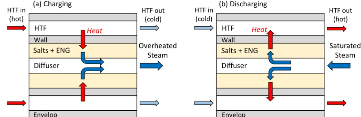
143
• Thermal integration (Thermal Int.): during the charging stage, water vaporsteam (500 °C, 144
1 bar) released from the TCES reactor is partially condensed in a heat exchanger to 145
preheat the working fluid of the Rankine cycle, then completely condensed by a 146
condenser and stored as the saturated liquid (100 °C, 1 bar) in a separate water reservoir. 147
During the discharging stage, steam extracted from the turbine of the power cycle is used 148
to vaporize the stored liquid water to the saturated vapor (100 °C, 1 bar), which will then 149
enter into the TCES reactor for exothermic reaction. The Rankine cycle and the TCES 150
circuit are thermally coupled with each other but without direct mass contact or exchange 151
(as shown in Fig. 3 of [Pelay, 2019]Fig. 2a). 152
153
• Mass integration (Mass Int.): the high temperature water vaporsteam generated in the 154
TCES reactor during the charging stage is stored as the saturated water (41 °C, 0.008 155
MPa) in a water reservoir shared with the Rankine cycle. During the discharging stage, the 156
stored liquid water is firstly pressurized by a pump and then evaporated into saturated 157
vapor (100 °C, 0.1 MPa) by high temperature extracted steam from the Turbine. For this 158
concept, the Rankine power cycle and the TCES circuit are coupled and share the same 159
working fluid with mass exchange (as shown in Fig. 2b Fig. 4 of [Pelay, 2019]). 160
161
• Turbine integration (Turbine Int.): during the charging stage, high temperature water
162
vaporsteam (500 °C, 1 bar) from the TCES reactor passes through an additional turbine
163
to valorize a part of its thermal energy as power production. The condensed water 164
(41.5 °C, 0.1 MPa) is stored in a separate water reservoir. The discharging stage is the 165
same as that of the Thermal Int. The principal Rankine circuit and the TCES circuit are 166
completely independent of each other during the charging stage (no heat or mass 167
exchange) and thermally coupled during the discharging stage (as shown in Fig. 2c Fig.
168 5 of [Pelay, 2019]). 169 170 Solar irradiation Fluxes Heliostats Open Feed water Heater Open Feed water Heater Central receiver Charging stage Discharging stage (a) Thermal integration concept
(b) Mass integration concept
(c) Turbine integration concept
Turbine 1 Condenser 1 Pump 1 Pump 2 Steam generator Water reservoir Condenser 2 TCES reactor Heat exchanger 1 Water reservoir Pump 1 Pump 2 Condenser 1 TCES reactor Heat exchanger 2 Turbine 1 Solar irradiation Fluxes Heliostats Central receiver TCES reactor Steam generator Turbine 1 Condenser 1 Water reservoir Condenser 2 Pump 1 Pump 2 Heat exchanger 1 Throttle valve TCES reactor Turbine 1 Condenser 1 Heat exchanger 2 Pump 2 Pump 1 Water reservoir Open Feed water Heater Pump 3 Charging stage Discharging stage Solar irradiation Fluxes Heliostats Open Feed water Heater Open Feed water Heater Central receiver Charging stage Discharging stage Turbine 1 Condenser 1 Pump 1 Pump 2 Steam generator Water reservoir Condenser 2 TCES reactor Water reservoir Pump 1 Pump 2 Condenser 1 TCES reactor Heat exchanger 2 Turbine 1 Turbine 2 Pump 3 Pressurized air as HTF Simulation boundary Solar tower Simulation boundary Simulation
boundary Simulation boundary
Solar tower Solar tower Pressurized air as HTF Pressurized air as HTF Simulation
boundary Simulation boundary
Figure 2. Schematic view of the SPT plant with TCES integration. (a) Thermal Int. concept; (b) Mass Int.
172
concept; (c) Turbine Int. concept. Adapted from [Pelay, 2019]
173 174
Detailed description of the three proposed Int. concepts as well as their performance 175
modelling based on static energy and exergy analyses can be found in our earlier work [Pelay, 2019]. 176
177 178 179 180
Table 1. Component model of the CSP plant with TCES integration used for the dynamic modeling
Component (Name) Library/Reference Modeling assumptions Features
Steam turbine
(SteamTurbine) ThermoCycle [Quoilin, 2017] - No thermal inertia - Constant Isentropic efficiency - Simple and robust - The Stodola’s law with partial arc admission permets the modeling of a gas expansion without sizing the turbine [Altés Buch, 2014]
Open water tank
(OpenTank) ThermoCycle [Quoilin, 2017]
A heat exchange port with the outside is added to model the heat loss
- Dynamic energy and mass conservation model - Constant outside pressure
- Inlet/outlet fluid at liquid state
- Simple and robust
- Constant pressure inside the tank Closed water tank
(Tank_PL) ThermoCycle [Quoilin, 2017] - Dynamic energy and mass conservation model - Constant outside pressure - Saturated outlet fluid
- No heat exchange with the outside
- A closed tank with a variable pressure inside - Inlet fluid can be a mixture of liquid and vapor Pump
(Pump) ThermoCycle [Quoilin, 2017] - Non-dynamic model - No heat loss - No thermal inertia
- Constant isentropic and mechanic efficiencies - Inlet/outlet fluid at liquid state
- Simple and robust - Variable rotation speed
Compressor (Compressor)
ThermoCycle [Quoilin, 2017] - Non-dynamic model - No heat loss - No thermal inertia
- Constant isentropic and mechanic efficiencies - Inlet fluid at gaseous state
Throttle valve
(Valve) ThermoCycle [Quoilin, 2017] - Non-dynamic model - No heat loss - Incompressible fluid
- Quadratic pressure loss for turbulent flow
- Non-linear equations generated by quadratic friction coefficient
Linear valve
(LinearValve) Modelica [Altés Buch, 2014] - Non-dynamic model - No heat loss - Incompressible fluid - Linear pressure drop
- Simple and robust - A no-return option for fluid Three way valve
(Three-way valve) Modelica Buildings library [MBL, 2018] - Non-dynamic model - No heat loss - Linear pressure drop
- Relatively simple control
- Presence of a dead volume preventing sudden pressure variations
TCES reactor
(Reactor) In-house
Appendix A1
- Uniform temperature in the composite - Uniform temperature in the wall - Uniform temperature in the fluid
- Entering vapor is instantly at composite temperature
- Sensitive to pressure variations
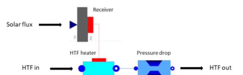
- Complicated to simulate several reactor in parallel Solar receiver
(Solar_Rec) In-house
Appendix A2
- No heat loss - No thermal inertia - Gaseous entering fluid
- Uniform temperature in the solar receiver
- Constant convective heat transfer coefficient - Dynamic model
Component (Name) Library/Reference Modeling assumptions Features Condenser
(CrossCondenser) [Altés Buch, 2014] - Constant temperature of cooling fluid - Fluid to be cooled is treated as a mixture of liquid and vapor - No sub-cooling at the outlet of condenser
- No heat loss - No inertia
- No liquid stored in the condenser
- Variable heat transfer coefficient - Discretized model on cold side
- Possibility to be coupled with a tank at the exit of the hot side - Very sensitive to pressure variations
Condenser
(Tank_Condenser) ThermoCycle [Quoilin, 2017] Based on the Tank model, heat transfer between hot and cold fluids is added in the conservation energy equation
- Dynamic model
- Wall temperature equals to the hot fluid temperature - Uniform temperature of hot fluid
- Fixed outlet temperature of cold fluid - No sub-cooling
- Compressible hot fluid - No heat loss
- Overestimated heat transfer surface area
- Very robust when coupled with a PID system - Condenser with an integrated tank
Evaporator
(Simplified_Evaporator) In-house
Appendix A3
- Incompressible fluid - No heat loss
- Fixed hot fluid outlet temperature
- Extremely robust - Very fast simulations Evaporator
(Tank_Boiler) ThermoCycle [Quoilin, 2017]
Based on the Tank model, heat transfer between hot and cold fluids is added in the conservation energy equation
- Dynamic model
- Wall temperature equals to the cold fluid temperature - Uniform temperature of cold fluid
- Fixed outlet pinch temperature - No over-heating
- Compressible cold fluid - No heat loss
- Overestimated heat transfer surface area
- Extremely robust Heat exchanger (Simplified_Heat_Exchanger) In-house Appendix A4 - Incompressible fluid - No heat loss
- Fixed pinch temperature
- Extremely robust - Very fast simulations Heat exchanger
(Hx1DInc) ThermoCycle [Quoilin, 2017] - Dynamic model - Uniform velocity on the cross section - Incompressible cold fluid
- Negligible longitudinal heat transfer - No heat loss
- Precise discretized model
2.2. Mathematic model for individual component
185186
Object-oriented Modelica modeling language is used for this study, enabling the description 187
of transient behaviors by models based on differential, algebraic and discrete equations. The 188
conservative equations of heat and mass transfer are firstly formulated for each component of the 189
CSP plant. These mathematic models are then coupled together to represent the whole CSP plant 190
with TCES integration. The resulting system of equations is solved at each time step by the DASSL 191
(Differential Algebraic System Solver) integration algorithm of Dymola solver [Dassault, 2011]. 192
Special attention is given to the initialization of simulations for such a complex system with 193
algebraic loops. 194
195
Too complex model for each individual component is difficult to be solved and coupled 196
together while a simpler model ignoring too many details may not be enough precise. A compromise 197
has thus to be reached between the accuracy and the complexity. Moreover, a global view of the 198
CPS plant to be simulated is also indispensable so as to identify the limiting factors (i.e. components 199
having the highest thermal inertia) for reasonable simplifications on les impacting components. 200
201
For most of the components, existing models in the Dymola library or in the literature are 202
adopted, with some necessary modifications. For the key components of the plant (e.g., solar 203
receiver, TCES reactor), their models are developed in house based on the proposed design and sizing. 204
Table 1 recapitulates the mathematical model used for every component, together with the modeling 205
assumptions of each. Note that for turbomachines (turbines, pumps and compressor), constant
206
coefficients (isentropic and volumetric efficiencies) were used, without taking into account the
207
partial load operation curves. Other components were sized for a nominal case covering all the
208
partial load scenarios and/or integrating variable coefficients. Detailed descriptions of the in-house
209
developed models can be found in Appendix A of this paper. 210 211 212
2.3. Operational mode
213 214Two clear sunny days (one in summer and another in winter) have been selected at eastern 215
Pyrenees (42.497N, 1.959E) where the Themis power plant is located [Larrouturou, 2014] have been
216
selected. The average Direct Normal Irradiance (DNI) curves [PVGIS] during the day are shown on
217
Fig. 13. For the summer day, the sunrise occurs at 5h07 and sunset at 18h37 whereas for the winter
218
day, the sunrise occurs at 7h52 and sunset at 15h52. The solar power Psol (W·m-2) based on the DNI
219
data is described by Eqs. (2-3) and will be used as inputs for each time step t (s) of the dynamic 220
simulations. Note that the short DNI variation due to clouds has not been taken into account.
221 222
For a typical summer day: 223 𝑷𝑷𝒔𝒔𝒔𝒔𝒔𝒔= ⎩ ⎨ ⎧𝒊𝒊𝒊𝒊 𝟏𝟏𝟏𝟏𝟏𝟏𝟏𝟏𝟏𝟏 < 𝒕𝒕 (𝒔𝒔)< 𝟔𝟔𝟔𝟔𝟏𝟏𝟏𝟏𝟏𝟏 ; −4.985809 × 10𝒊𝒊𝒊𝒊 𝒕𝒕 (𝒔𝒔)−24< 𝟏𝟏𝟏𝟏𝟏𝟏𝟏𝟏𝟏𝟏 ; 0× 𝑡𝑡6+ 1.264474 × 10⁻¹⁸× 𝑡𝑡5− 1.309668 × 10⁻¹³× 𝑡𝑡4 +7.086230 × 10⁻⁹× 𝑡𝑡3− 2.116637 × 10⁻⁴× 𝑡𝑡2+ 3.328676 × 𝑡𝑡 − 2.10949 × 10⁴ 𝒊𝒊𝒊𝒊 𝒕𝒕 (𝒔𝒔)> 𝟔𝟔𝟔𝟔𝟏𝟏𝟏𝟏𝟏𝟏 ; 0 (2) 224
For a typical winter day: 225
𝑷𝑷𝒔𝒔𝒔𝒔𝒔𝒔= ⎩ ⎨ ⎧𝒊𝒊𝒊𝒊 𝟏𝟏𝟏𝟏𝟐𝟐𝟏𝟏𝟏𝟏 < 𝒕𝒕 (𝒔𝒔)< 𝟓𝟓𝟔𝟔𝟏𝟏𝟏𝟏𝟏𝟏 ; −2.86954539 × 10𝒊𝒊𝒊𝒊 𝒕𝒕 (𝒔𝒔)−15< 𝟏𝟏𝟏𝟏𝟐𝟐𝟏𝟏𝟏𝟏 ; 0× 𝑡𝑡4+ 4.97529124 × 10⁻¹⁰× 𝑡𝑡3− 3.28214478 × 10⁻⁵× 𝑡𝑡2 + 9.75426171 × 10⁻¹× 𝑡𝑡 − 1,05104646 × 10⁴ 𝒊𝒊𝒊𝒊 𝒕𝒕 (𝒔𝒔)> 𝟓𝟓𝟔𝟔𝟏𝟏𝟓𝟓𝟔𝟔 ; 0 (3) 226 227 228
Figure 13. Average DNI for a typical summer and a winter day at eastern Pyrenees (42.497N, 1.959E) [PVGIS]
229 230 231
The basic production mode is firstly studied for three Int. concepts. The CSP plant is 232
expected to produce electricity continuously at a constant power output over the longest possible 233
period of time with the help of the TCES unit. Nevertheless, the continuous dynamic simulation of 234
the CSP plant for a whole day is difficult at this stage, due to the complicated initialization and 235
calculation instability. As a result, dynamic simulations have been performed for three separate 236
phases of the operational mode, as shown in Fig. 2 4 and explained in detail as follows. 237
238
• Phase 1: plant starting. At the beginning of a day, the solar power (Psol) is not enough to 239
run the Rankine power cycle at its nominal output (PRankine). This amount of solar energy 240
is used only for the TCES unit, i.e., to preheat the TCES reactor and to initiate the 241
endothermic reaction when the equilibrium reaction temperature (500 °C) is reached. 242
243
• Phase 2: nominal production. Once the solar power meets the need to run the Rankine 244
power cycle (Psol>PRankine), the nominal production of the CSP plant (phase 2) starts. The 245
TCES system is charged simultaneously by excessive amount of solar energy for later use. 246
247
• Phase 3: prolonged production. At the end of the day when the decreased solar power 248
becomes insufficient to run the Rankine power cycle at its nominal output (Psol<PRankine), 249
the TCES reactor begins to discharge to compensate the deficiency. The production of 250
CSP plant is prolonged owing to the stored solar energy in phases 1 and 2, until the TCES 251
reactor temperature (TR) falls below a threshold value fixed by users (e.g., 485 °C). The 252
cut-off temperature of the TCES reactor at the end of phase 3 is determined to equal to
253
485 °C, permitting still the overheated steam of the principal Rankine cycle at the outlet
254
of the evaporator rising to 480 °C. The heat loss of the TCES reactor overnight is
255
estimated to be negligible supposing that the TCES reactor is well-insulated.
256 257 258 0 200 400 600 800 0 2 4 6 8 10 12 14 16 18 20 22 24 DNI (W ·m -2) Time (h) Juillet Janvier Summer Winter
So lar p ow er (Pso l ) Time
Phase 1 Phase 2 Phase 3
PRankine Solar Power Minimum required solar power TCES Charging Production driven by the Rankine cycle Production by TCES discharging
259
Figure 24. Schematic view of the operational mode divided into 3 phases for the basic continuous production 260
mode 261
262
At the end of each phase, all the system’s variables (e.g., reactor temperature, receptor solar
263
receiver temperature, pressure in all points, chemical reaction progress) are recorded and transferred
264
to initiate the next phase. Moreover, phase 2 is delayed from the end of phase 1 because discretized 265
components used in the Rankine cycle are unstable to simulate at zero flowrate. Other simulations 266
of the Rankine cycle and more precisely of the evaporator showed that the Rankine cycle needs 15 267
minute to reach its nominal operation point. 268 269 270
2.4. Control strategy
271 272The proper operation of the CSP plant with TCES integration requires an adapted control 273
strategy to perform multiple controls of the installation. The widely-used PI or PID controllers have 274
been used owing to their robustness and high controlling efficiency. To determine the PID 275
parameters, the manual setup was used whenever possible for simple systems. Otherwise, the 276
Ziegler-Nichols reaction curve method was adopted [Das, 2014]. The controllers used in this study 277
are recapitulated in Table B1 of Appendix B2. 278
279
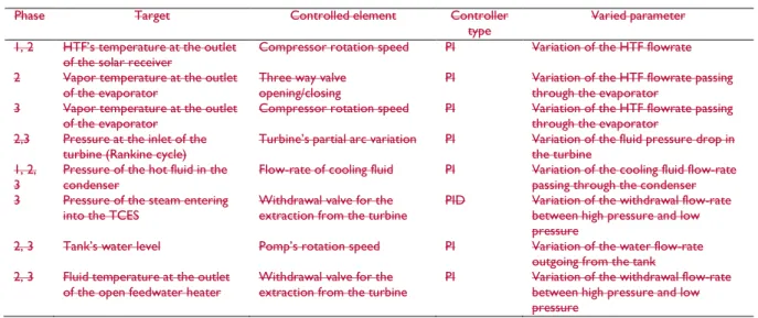
Table 2. List of all PID controllers
280 281
Phase Target Controlled element Controller
type Varied parameter
1, 2 HTF’s temperature at the outlet
of the solar receiver Compressor rotation speed PI Variation of the HTF flowrate
2 Vapor temperature at the outlet
of the evaporator
Three way valve opening/closing
PI Variation of the HTF flowrate passing
through the evaporator
3 Vapor temperature at the outlet
of the evaporator Compressor rotation speed PI Variation of the HTF flowrate passing through the evaporator
2,3 Pressure at the inlet of the
turbine (Rankine cycle) Turbine’s partial arc variation PI Variation of the fluid pressure drop in the turbine
1, 2,
3 Pressure of the hot fluid in the condenser Flow-rate of cooling fluid PI Variation of the cooling fluid flow-rate passing through the condenser
3 Pressure of the steam entering
into the TCES Withdrawal valve for the extraction from the turbine PID Variation of the withdrawal flow-rate between high pressure and low pressure
2, 3 Tank’s water level Pump’s rotation speed PI Variation of the water flow-rate
outgoing from the tank
2, 3 Fluid temperature at the outlet
of the open feedwater heater Withdrawal valve for the extraction from the turbine PI Variation of the withdrawal flow-rate between high pressure and low pressure
282 283
2.5. Sizing and simulation parameters
284The solar field (heliostats) has been sized so that the TCES reactor can be almost completely 286
charged (X=0.05) at the end the charging stage (phase 2) for a summer day. Note that the cosine
287
loss was not considered during the sizing, which may results in an underestimation of the required
288
solar field areas [Peng, 2013]. The solar field surface areas for different TCES integration concepts
289
are listed in Table 23. Details for the modeling of the solar receiver are provided in Appendix A2 of 290
this paper. 291
292
Table 23. Sizing of the solar field for different TCES integration concepts 293
294
Thermal Int. Mass Int. Turbine Int. Solar field area (m²) 1 033 000 1 065 500 908 000 295
296
The cut-off temperature of the TCES reactor at the end of phase 3 is determined to equal to
297
485 °C, permitting still the overheated steam of the principal Rankine cycle at the outlet of the
298
evaporator rising to 480 °C. The heat loss of the TCES reactor overnight is estimated to be negligible
299
supposing that the TCES reactor is well-insulated.
300 301
The nomenclature, the Pparameter values and variables fixed by the user and controlled by
302
the PID controllers for the dynamic simulation can be found in Tables B2-B5 of Appendix B4-7. 303
Note that the power parasitic consumption is taken into account in the TCES reactor (stoichiometric
304
reaction coefficient) and in the pumps, the turbines and the compressor (isentropic and volumetric
305
efficiency). For other components, no power parasitic consumption is considered.
306 307
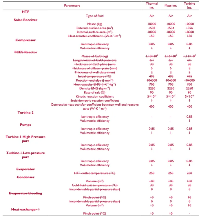
Table 4. Parameter values for different components of the system
308 309
Parameters Thermal Int. Mass Int. Turbine Int.
HTF
Type of fluid Air Air Air
Solar Receiver
Masse (kg) 10000 10000 10000
External surface area (m2) 1503 1534 1396
Internal surface area (m2) 18000 18000 18000
Heat transfer coefficient (W·K-1·m-2) 150 150 150
Compressor
Isentropic efficiency 0.85 0.85 0.85
Volumetric efficiency 1 1 1
TCES Reactor
Masse of CaO (kg) 1.10×10⁷ 1.16×10⁷ 1.11×10⁷
Length/width of CaO plate (m) 6/1 6/1 6/1
Thickness of CaO plate (mm) 30 30 30
Thickness of diffuser plate (mm) 5 5 5
Thickness of wall plate (mm) 2 2 2
Initial temperature (°C) 495 495 495
Reaction enthalpy (J·mol-1) 104000 104000 104000
Heat capacity ENG (J·K-1·kg-1) 700 700 700
Density ENG (kg·m-3) 2250 2250 2250
Rate of salt (%) 90 90 90
Kinetic reaction coefficient 5×10⁻³ 5×10⁻³ 5×10⁻³
Stoichiometric reaction coefficient 1 1 1
Convective heat transfer coefficient between wall and reactive
salts (W·K-1·m-2) 400 400 400 Turbine 2 Isentropic efficiency - - 0.85 Volumetric efficiency - - 1 Pumps Isentropic efficiency 0.85 0.85 0.85 Volumetric efficiency 1 1 1
Parameters Thermal Int. Mass Int. Turbine Int.
Turbine 1 High Pressure part
Isentropic efficiency 0.85 0.85 0.85
Volumetric efficiency 1 1 1
Turbine 1 Low pressure part Isentropic efficiency 0.85 0.85 0.85 Volumetric efficiency 1 1 1 Evaporator HTF outlet temperature (°C) 250 250 250 Condenser Volume (m3) 100 100 100
Cold fluid exit temperature (°C) 30 30 30
Incondensable partial pressure (bar) 0 0 0
Evaporator bleeding
Pinch point (°C) 10 10 10
Incondensable partial pressure (bar) 0 0 0
Volume (m3) 10 10 10
Heat exchanger 1
Pinch point (°C) 10 10 -
310 311
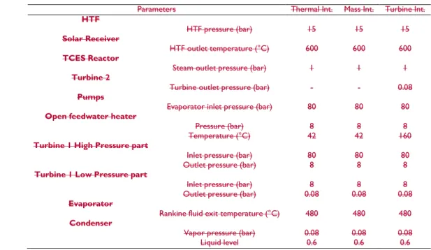
Table 5. Variables fixed by user - Phase 1
312 313
Parameters Thermal Int. Mass Int. Turbine Int.
HTF
HTF pressure (bar) 15 15 15
Solar receiver
HTF exit temperature (°C) 600 600 600
TCES reactor
Steam exit pressure (bar) 1 1 1
Turbine 2
Turbine exit pressure (bar) - - 0.08
314 315
Table 6. Variables fixed by user - Phase 2
316 317
Parameters Thermal Int. Mass Int. Turbine Int.
HTF
HTF pressure (bar) 15 15 15
Solar Receiver
HTF outlet temperature (°C) 600 600 600
TCES Reactor
Steam outlet pressure (bar) 1 1 1
Turbine 2
Turbine outlet pressure (bar) - - 0.08
Pumps
Evaporator inlet pressure (bar) 80 80 80
Open feedwater heater
Pressure (bar) 8 8 8
Temperature (°C) 42 42 160
Turbine 1 High Pressure part
Inlet pressure (bar) 80 80 80
Outlet pressure (bar) 8 8 8
Turbine 1 Low Pressure part
Inlet pressure (bar) 8 8 8
Outlet pressure (bar) 0.08 0.08 0.08
Evaporator
Rankine fluid exit temperature (°C) 480 480 480
Condenser
Vapor pressure (bar) 0.08 0.08 0.08
Liquid level 0.6 0.6 0.6
318 319
Table 7. Variables fixed by user - Phase 3
320 321
Parameters Thermal Int. Mass Int. Turbine Int.
HTF
HTF pressure (bar) 15 15 15
TCES Reactor
Steam inlet pressure (bar) 1 1 1
Steam state Saturated Saturated Saturated
Pumps
Evaporator enter pressure (bar) 80 80 80
Open feedwater heater
Pressure (bar) 8 8 8
Temperature (°C) 42 42 160
Turbine 1 High Pressure Part
Inlet pressure (bar) 80 80 80
Outlet pressure (bar) 8 8 8
Turbine 1 Low Pressure Part
Inlet pressure (bar) 8 8 8
Outlet pressure (bar) 0.08 0.08 0.08
Evaporator
Rankine fluid outlet temperature (°C) 480 480 480
Condenser
Vapor pressure (bar) 0.08 0.08 0.08
Liquid level 0.6 0.6 0.6
Incondensable partial pressure (bar) 0 0 0
Heat exchanger 2
Inside pressure (bar) 1 1 1
Liquid level 0.6 0.6 0.6
322 323
3. Results and discussion for the basic production scenario
324 325
This section shows main results of the dynamic simulation for summer and winter days. 326
Recall that the solar field and relevant components have been sized to offer an optimal operation 327
for a typical summer day and for the basic continuous production scenario. 328 329 330
3.1. Charging/discharging duration
331 332From Fig. 3 5 one may observe that there is a slight difference on the charging/discharging 333
durations for different Int. concepts. Indeed, due to their conceptions, all the systems do not need 334
the same minimal amount of energy to operate. For example, the Turbine Int. concept would benefit 335
an earlier start and delayed stop, thereby rendering a relatively longer charging and a shorter 336
discharging in summer. In winter, these durations are significantly lower than those of summer for 337
all the Int. concepts studied. The CSP plant does not have the necessary solar power to decompose 338
all the TCES materials: the TCES reactor is largely oversized for a typical "winter" day. 339
340
341
Figure 35. Charging/discharging durations for different integration concepts 342 0 2 4 6 8 10 12 14 16 18
Thermal Int. Mass Int. Turbine Int.
D ur at io n ( h)
Charging summer Discharging summer Charging winter Discharging winter
343 344
3.2. Electricity consumption/production
345346
In order to make an easier comparison between the three integration concepts, the ratios of 347
the electricity consumption (whole plant or Rankine cycle) to the electricity production have
348
beenare represented on Fig. 46.
349 350
351
Figure 46. Ratio of electricity consumption to production for the CSP plant with different TCES integration 352
concepts (MW.helconsumed/MW.helproduced)
353 354
The electricity energy is mainly used to run the compressor for the HTF (pressurized air) in 355
the solar circuit and the pumps in the Rankine cycle. In summer, the Rankine cycle electricity 356
consumption is just about one tens of the overall electricity consumption. And in winter, the 357
proportion is one third. It can be noticed from Fig. 4 6 that the electricity consumption for the 358
Rankine cycle is approximately the same for all the integration concepts (about 0.01 359
MW.hconsumed/MW.hproduced for both summer and winter). This is because the electricity consumption 360
for running the pumps mainly depends on the mass flow-rate of the Rankine cycle’s HTF, which is 361
almost identical for all the integration concepts because of the same nominal production power of 362
100 MWel. 363
364
The global electricity consumption of the CSP plant is about 12% of the total electricity 365
production for a typical summer day whereas for a typical winter day, the proportion is about 3%. 366
No big difference between the three Int. concepts has beenis observed. Meanwhile, the noticeable 367
difference in global consumption between summer and winter is mainly due to the different mass 368
flow-rate of HTF (pressurized air) in the solar circuit. Higher amount of solar energy available in 369
summer needs to be transported by the HTF, resulting in higher electricity consumption in the air 370
compressor. 371
372
Several methods may be employed to decrease the electricity consumption of the compressor 373
(thus the global electricity consumption). A simple way is to raise the upper temperature limit of 374
the HTF (700 °C in the current study) so as to reduce the required HTF mass flow-rate. However, 375
the equipment used for the solar circuit should resist to higher temperature in this case. Another 376
way is to use a liquid HTF having a higher heat capacity (e.g., molten salts, synthetic oils) instead 377 0.00 0.02 0.04 0.06 0.08 0.10 0.12 0.14 0.16
Thermal Int. Mass Int. Turbine Int.
R atio o f e le ctr ic ity c on su m pti on to p ro du ct io n
Global summer Rankine summer Global winter Rankine winter
of the pressurized air. But it will bring new problems such as the solidification of molten salts and 378
the higher environmental impacts [Batuecas, 2017]. 379 380 381
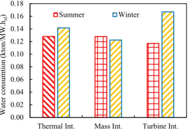
3.3. Water consumption
382 383The water consumption refers to the quantity of cooling water for the condensers of the CSP 384
plant, one for the Rankine cycle and another for the TCES unit. Note that the cooling water inlet 385
temperature is 15 °C and the outlet temperature is fixed at 30 °C (maximum allowable temperature 386
in France) [Khalanski, 1996; MTES, 1998]. Figure 5 7 shows the water consumption (kton) per 387
MW.hel produced for different Int. concepts of the CSP plant. 388
389
For a typical summer day, the Turbine Int. concept has the lowest water consumption (0.12 390
kton/MW.hel) because of its highest turbine bleeding at the nominal power that decreases the water 391
consumption for the condenser of the Rankine cycle. However, for a typical winter day, its water 392
consumption is the highest (0.17 kton/MW.hel) compared to the Thermal Int concept (0.14 393
kton/MW.hel) or the Mass Int. concept (0.12 kton/MW.hel). In winter, the charge charging of the 394
TCES reactor is more important for the Turbine Int. concept, which induces a higher water 395
consumption. CSP plants are usually installed in desert/remote areas close to the equator (e.g., USA, 396
Morocco, Spain, MENA [Pelay, 2017a; b]) with summer climate in principle. The Turbine Int. 397
concept seems to be more beneficial regarding its lower water consumption during summer. 398
399
400
Figure 57. Water consumption (kton/MW.hel) of the CSP plant with different TCES integration
401 concepts 402 403 404
3.4. Energy efficiency
405 406The Rankine efficiency (𝜂𝜂𝑅𝑅𝑅𝑅𝑅𝑅𝑅𝑅𝑅𝑅𝑅𝑅𝑅𝑅) is defined as the efficiency of the Rankine cycle without
407
considering the solar circuit whereas the global efficiency (𝜂𝜂𝐺𝐺𝐺𝐺𝐺𝐺𝐺𝐺𝑅𝑅𝐺𝐺) represents the efficiency of the
408
whole CSP plant. They are calculated following the Eqs. (4) and (5). 409 𝜂𝜂𝑅𝑅𝑅𝑅𝑅𝑅𝑅𝑅𝑅𝑅𝑅𝑅𝑅𝑅 =�𝑊𝑊𝑇𝑇,𝐶𝐶− 𝑊𝑊𝑃𝑃,𝐶𝐶(𝑄𝑄�. 𝐻𝐻𝐶𝐶+ �𝑊𝑊𝑇𝑇,𝐷𝐷− 𝑊𝑊𝑃𝑃,𝐷𝐷�. 𝐻𝐻𝐷𝐷 𝑆𝑆𝐺𝐺+ 𝑄𝑄𝑅𝑅). 𝐻𝐻𝐶𝐶 (4) 0.00 0.02 0.04 0.06 0.08 0.10 0.12 0.14 0.16 0.18
Thermal Int. Mass Int. Turbine Int.
W at er c on su m tio n ( kto n/MW .hel ) Summer Winter
𝜂𝜂𝐺𝐺𝐺𝐺𝐺𝐺𝐺𝐺𝑅𝑅𝐺𝐺 =�𝑊𝑊𝑇𝑇,𝐶𝐶− 𝑊𝑊𝑃𝑃,𝐶𝐶− 𝑊𝑊𝐶𝐶𝑃𝑃,𝐶𝐶(𝑄𝑄�. 𝐻𝐻𝐶𝐶+ �𝑊𝑊𝑇𝑇,𝐷𝐷− 𝑊𝑊𝑃𝑃,𝐷𝐷− 𝑊𝑊𝐶𝐶𝑃𝑃,𝐷𝐷�. 𝐻𝐻𝐷𝐷 𝑆𝑆𝐺𝐺+ 𝑄𝑄𝑅𝑅). 𝐻𝐻𝐶𝐶
(5)
with: WT, the energy produced by the turbines (W) 410
WP, the energy consumed by the pumps (W) 411
QSG, the energy consumed by the Rankine cycle’s steam generator (W) 412
QR, the energy consumed by the thermochemical reactor (W) 413
WCP, the energy consumed by the compressor (W) 414
H, the duration (h) 415
The indices C and D indicate the charging and the discharging stage, respectively. 416
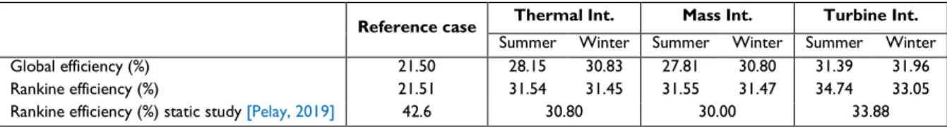
417
Table 3 8 lists the simulated values of global and Rankine energy efficiencies for different 418
Int. concepts during typical summer and winter days. It can be easily observed that the Turbine 419
Int. concept has the highest global energy efficiency: 31.39% for summer and 31.96% for winter, 420
respectively. The option of using a second turbine to valorize the waste heat of high temperature 421
vapor steam from the TCES reactor makes it attractive. Despite that the solar field is designed for
422
summer operation, the winter’s global efficiency is higher than that of summer for all the Int. 423
concepts. In fact, the heat storage in the TCES reactor has two parts: thermochemical reaction heat 424
and the sensible heat of the reactive salts and the reactor body. The TES by thermochemical 425
reaction is generally less efficient than the sensible storage due to the heat loss of the superheated 426
vapor steam extracted from the TCES reactor during its condensation. For a typical winter day, the
427
TCES reactor is only partially charged: approximately 20% of the Ca(OH)2 has been decomposed 428
whereas it is about 80% for summer. This makes the contribution of the “sensible part” more 429
important for the total TES, leading to the higher global energy efficiency of the CSP plant. Note 430
that the reference case (without TES) has a significantly lower global energy efficiency of 21.50%. 431
Indeed, an important amount of solar radiation received by the central solar receiver cannot be 432
converted into heat and is thus lost. 433
434
Table 38. Simulation results on energy efficiency of the CSP plant for typical summer and winter days (basic 435 production mode) 436 437 438 439
Generally speaking, the Rankine efficiency is slightly higher than the global efficiency by 440
neglecting the losses in the solar circuit. The values of Rankine efficiency obtained by the dynamic 441
study are close to those obtained in the static study [Pelay, 2019] for all the three Int. concepts (less 442
than 1% difference). However, the Rankine efficiency of the reference case has halved from 42.6% 443
to 21.51%. This is because during the static study, the amount of solar energy was considered as 444
constant all along the day. While in this dynamic study, it is varied all the time. This variability 445
induces a large amount of lost energy. 446
Reference case Thermal Int. Mass Int. Turbine Int.
Summer Winter Summer Winter Summer Winter
Global efficiency (%) 21.50 28.15 30.83 27.81 30.80 31.39 31.96
Rankine efficiency (%) 21.51 31.54 31.45 31.55 31.47 34.74 33.05
447 448
4. Peak production mode
449 450
In this section, the dynamic simulation results for a peak production mode are reported. 451
Contrary to the basic continuous production scenario, the peak production mode aims at a massive 452
electricity production within one or several short periods of time when the electricity selling price is 453
the highest on the spot market [Tapachès, 2019]. It is thus interesting to compare the same TCES 454
Int. concept for two different modes of production. The Turbine Int. concept has been selected for 455
this purpose because it enables the waste heat recovery of overheated vapors via the second turbine 456
when the principal Rankine cycle is not working. 457
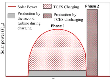
458
The operation mode is shown in Fig. 68. During phase 1, the Rankine cycle is at the stop 459
state without electricity production. The TCES reactor is charged and a part of the waste heat of 460
the superheated vapor steam is valorized as electricity production via the second turbine in the 461
TCES circuit. During phase 2 (peak hour but insufficient sunshine), the stored heat will be all 462
discharged to run the Rankine cycle at about 1000 MWel (10 times of the nominal power), in order 463
to realize a peak power production within about 1 hour. 464 465 So lar p ow er (Pso l ) Time Phase 1 Phase 2
Solar Power TCES Charging Production by TCES discharging Production by the second turbine during charging 466
Figure 68. Schematic view of the operational mode for the peak production mode 467
468 469
Table 4 9 summarizes all the mains simulation results for a typical summer day under peak 470
and basic production modes. The charging duration of 12.7 hours corresponds to the total sunshine 471
duration (Fig. 18). The discharging duration (1.1 hour) is determined by the size of the TCES reactor 472
which is the same as that for the basic production mode. The second turbine of the TCES circuit 473
produces 550 MW.hel during the charging (Phase 1) while the Rankine cycle generates 1002 MW.hel 474
during the peak hour. 475
476
Table 49. Dynamic simulations results of Turbine Int. concept for a typical summer day in basic and peak 477
production modes 478
479
Efficiency Global efficiency (%) 28.15 17.89 Rankine efficiency (%) 31.54 27.96 Storage Charge duration (h) 12.3 12.7 Discharge duration (h) 13.06 1.1
Energy produced/ consumed
Global energy produced (MW.h) 2601 1552
Global energy consumed (MW.h) 304 567
Rankine energy consumed (MW.h) 27 12
Water consumption
Global water consumption (kton) 333 219
480 481
The Rankine cycle electricity consumption (12 MW.hel) only represents a small proportion 482
(2%) of the high global electricity consumption (567 MW.hel). The latter (0.37 MW.hel, 483
consumed/MW.hel, produced) is nearly four times higher than that of the basic production mode (0.09 484
MW.hel, consumed/MW.hel, produced). This is because the mass flow-rate of HTF has increased by a factor 485
of 10 (16000 kg·s-1 instead of 1500 kg·s-1), resulting in much higher pressure loss in the central solar 486
receiver thus higher electricity consumption of the compressor. The water consumption is also more 487
important for the peak production mode (0.14 kton/MW.hel, produced) compared to that for the basic 488
production mode (0.12 kton/MW.hel, produced). 489
490
The Rankine and global energy efficiency is respectively 17.89% and 27.96%, both lower 491
than those for the basic production mode. Regarding the energy efficiency and environmental 492
impacts, the peak production mode seams less interesting than the basic mode. A techno-economic 493
study considering the variation of the selling electricity price on the spot market is necessary to 494
better evaluate its potential. 495
496 497
5. Conclusion
and prospects
498 499
In this study, the dynamic simulation of a CSP plant with TCES system integration have 500
been performed. The Dymola environment has been used with component models existing in the 501
library or developed in-house. Both the basic continuous production mode and the peak production 502
mode have been investigated. Based on the results obtained, main conclusions can be summarized 503
as follows. 504
505
• TES integration is needed to increase the output of a CSP plant. Among the three TCES Int. 506
concepts proposed, the Turbine Int. concept has the best global efficiency (31.39% for 507
summer; 31.96% for winter). 508
509
• The TCES unit and solar field sized for a typical summer day will be largely oversized when 510
used for a typical winter day. 511
• The global electricity consumption of the CSP plant with TCES integration is about 12% of 513
the total electricity production for a typical summer day and about 3% for a typical winter 514
day. 515
516
• The water consumption of the CSP plant with TCES integration is about 0.12 kton/MW.hel 517
for a typical summer day. For a typical winter day, the water consumption of the Turbine 518
Int. concept is the highest (0.17 kton/MW.hel) compared to the Thermal Int concept (0.14 519
kton/MW.hel) or the Mass Int. concept (0.12 kton/MW.hel). 520
521
• The peak production mode is achievable by using the Turbine Int. concept. An increased 522
nominal power by a factor of 10 could be reached by discharging the stored heat within one 523
hour. However, a lower global efficiency (17.89%) is rendered due to the higher electricity 524
consumption of the air compressor in the solar circuit. It will then be interesting to carry
525
out a techno-economic study for different integrations and modes of production
526 527
One limitation of the current study is that the simulations are based on two perfect summer
528
and winter days while the effect of cloud passages has not been considered yet. Nevertheless, the
529
simulations showed that the large thermal inertia of the TCES unit, owing to the great quantity of
530
stainless steel (~1.2×10⁷ kg) and reactive salts (~1.1×10⁷ kg) involved, can allow a quick
531
charging/discharging switch and maintain a constant output of the Rankine power cycle. A future
532
work using real DNI curves surveyed for some typical cloudy days will provide more details on
533
influence of the short DNI variation.
534 535
Another simplification made is that the DNI value has not been corrected with the cosine
536
loss, which could have a non-negligible impact on the simulation results: about 5% in summer and
537
30% in winter based on the estimation of Peng et al., [2013]. Taking into account the cosine loss
538
would increase the size of solar field (designed for a perfect summer day) and thereby decrease the
539
electricity production of the winter day. This matter of concern should be addressed in the future
540
studies.
541 542
It should be noted that this study has focused on the energy modeling and dynamic
543
simulation of the CSP plant, under the basic and peak operation modes. The improvement of the
544
models used for the simulations and their parameter remains an important objective. A real power
545
parasitic consumption of the turbomachines (turbines, pumps and compressor) would be obtained
546
with variables isentropic efficiencies. Futures experiments will also enable the use of a real
547
stoichiometric reaction coefficient for the thermochemical reactor. Furthermore, a techno-economic
548
assessment is also suggested in the future study to further understand the usability and the
cost-549
effectiveness of the proposed TCES integration concepts. Recent advances on the techno-economic
550
issue can be found in Refs [Salas, 2018; Tapachès; 2019].
551 552 553 554
Acknowledgement
555556
This work is supported by the French ANR within the project In-STORES (ANR-12-557
SEED-0008). 558
559
Appendix A. Detailed description of the in-house developed models
560 561
Appendix B. Parameter values and variables fixed by the user for the dynamic simulation
562 563 564
Nomenclature
565 566 Latin letters 567H charging or discharging time, h 568
P power, W
569
Q heat exchange rate, W
570
W work exchange rate, W
571 T temperature, K 572 t time, s 573 X reaction progress, (-) 574 575 Greek symbols 576 η energy efficiency 577
∆hR specific reaction heat, kJ.kg-1 578 579 Subscripts 580 C charging stage 581 CP compressor 582 D discharging stage 583 el electricity 584
Global Whole system 585
P pump
586
R reactor
587
Rankine Rankine circuit 588 SG steam generator 589 sol solar 590 T turbine 591 592 593
References
594 595
Albanakis, C., Missirlis, D., Michailidis, N., Yakinthos, K., Goulas, A., Omar, H., Tsipas, D., Granier, B. (2009). 596
Experimental analysis of the pressure drop and heat transfer through metal foams used as volumetric receivers 597
under concentrated solar radiation. Experimental Thermal and Fluid Science, 33(2), 246–252. 598
https://doi.org/10.1016/j.expthermflusci.2008.08.007 599
600
Alovisio, A., Chacartegui, R., Ortiz, C., Valverde, J.M., Verda, V. (2017). Optimizing the CSP Calcium Looping 601
integration for Thermochemical Energy Storage. Energy Conversion and Management, 136, 85–98. 602
doi:10.1016/j.enconman.2016.12.093. 603
604
Altés Buch, Q. (2014). Dynamic modeling of a steam Rankine Cycle for Concentrated Solar Power applications. 605
Master thesis, University of Liege. 606
607
Alva, G., Lin, Y., & Fang, G. (2018). An overview of thermal energy storage systems. Energy. 144, 341-378. 608
https://doi.org/10.1016/j.energy.2017.12.037 609
610
Batuecas, E., Mayo, C., Díaz, R., & Pérez, F. J. (2017). Life Cycle Assessment of heat transfer fluids in parabolic 611
trough concentrating solar power technology. Solar Energy Materials and Solar Cells, 171, 91–97. 612
https://doi.org/10.1016/j.solmat.2017.06.032 613
614
Cabeza, L. F., Solé, A., Fontanet, X., Barreneche, C., Jové, A., Gallas, M., Fernández, A. I. (2017). 615
Thermochemical energy storage by consecutive reactions for higher efficient concentrated solar power plants 616
(CSP): Proof of concept. Applied Energy, 185, 836–845. https://doi.org/10.1016/j.apenergy.2016.10.093 617
618
Das D., Sinha N., Roy K., Automatic generation control of an organic Rankine cycle solar-thermal/wind-619
diesel hybrid energy system. Energy technology, 2, 721-731. 620
https://onlinelibrary.wiley.com/doi/abs/10.1002/ente.201402024 621
622
Dassault Systèmes AB. (2011). User Manual. Dymola (Dynamic Modeling Laboratory) 623
624
Ding, W., Shi, H., Jianu, A., Xiu, Y., Bonk, A., Weisenburger, A., & Bauer, T. (2019). Molten chloride salts 625
for next generation concentrated solar power plants: Mitigation strategies against corrosion of structural 626
materials. Solar Energy Materials and Solar Cells, 193, 298–313. https://doi.org/10.1016/j.solmat.2018.12.020 627
628
Gimenez, P., & Fereres, S. (2015). Effect of Heating Rates and Composition on the Thermal Decomposition 629
of Nitrate Based Molten Salts. Energy Procedia, 69, 654–662. https://doi.org/10.1016/j.egypro.2015.03.075 630
631
IEA (2018). World Energy Outlook (WEO) 2018, International Energy Agency. ISBN: 978-92-64-30677-6. 632
633
IRENA (2018). Renewable Power Generation Costs in 2017. International Renewable Energy Agency. 634
https://www.irena.org/-/media/Files/IRENA/Agency/Publication/2018/Jan/IRENA_2017_Power_Costs_2018.pdf 635
636
Jarimi, H., Aydin, D., Yanan, Z., Ozankaya, G., Chen, X., & Riffat, S. (2019). Review on the recent progress 637
of thermochemical materials and processes for solar thermal energy storage and industrial waste heat recovery. 638
International Journal of Low-Carbon Technologies, 14, 44-69. https://doi.org/10.1093/ijlct/cty052
639 640
Khalanski, M., Gras, R. (1996). Rejets en rivières et hydrobiologie – Un aperçu sur l’expérience française. La 641
houille blanche. http://dx.doi.org/10.1051/lhb/1996046
642 643
Kuravi, S., Trahan, J., Goswami, D. Y., Rahman, M. M., & Stefanakos, E. K. (2013, August). Thermal energy 644
storage technologies and systems for concentrating solar power plants. Progress in Energy and Combustion Science. 645
https://doi.org/10.1016/j.pecs.2013.02.001 646
647
Larrouturou, F., Caliot, C., & Flamant, G. (2014). Effect of directional dependency of wall reflectivity and 648
incident concentrated solar flux on the efficiency of a cavity solar receiver. Solar Energy, 109(1), 153–164. 649
https://doi.org/10.1016/j.solener.2014.08.028 650
Lin, Y., Alva, G., & Fang, G. (2018). Review on thermal performances and applications of thermal energy 652
storage systems with inorganic phase change materials. Energy, 165, 685-708. 653
https://doi.org/10.1016/j.energy.2018.09.128 654
655
Liu, D., Xin-Feng, L., Bo, L., Si-quan, Z., & Yan, X. (2018). Progress in thermochemical energy storage for 656
concentrated solar power: A review. International Journal of Energy Research, 42, 4546-4561. 657
https://doi.org/10.1002/er.4183 658
659
Lu, W., Zhao, C. Y., & Tassou, S. A. (2006). Thermal analysis on metal-foam filled heat exchangers. Part I: 660
Metal-foam filled pipes. International Journal of Heat and Mass Transfer, 49(15–16), 2751–2761. 661
https://doi.org/10.1016/j.ijheatmasstransfer.2005.12.012 662
663
Martiensen, W., Warlimont, H. (2005). Springer hanbook of condensed matter and materials data. Springer 664
handbooks. eReference ISBN 978-3-540-30437-1.
665 666
Mazet, N., & Amouroux, M. (1991). Analysis of heat transfer in a non-isothermal solid-gas reacting medium. 667
Chemical Engineering Communications, 99(1), 175–200. https://doi.org/10.1080/00986449108911586
668 669
MBL (2018). Modelica Buildings library - Open source library for building energy and control systems. 670
http://simulationresearch.lbl.gov/modelica/index.html 671
672
Mohan, G., Venkataraman, M. B., & Coventry, J. (2019). Sensible energy storage options for concentrating 673
solar power plants operating above 600 °C. Renewable and Sustainable Energy Reviews, 107, 319-337. 674
https://doi.org/10.1016/j.rser.2019.01.062 675
676
MTES (1998). Ministère de la transition écologique et solidaire (1998). Circulaire du 06/06/53 relative au 677
rejet des eaux résiduaires par les établissements classés comme dangereux, insalubres ou incommodes en 678
application de la loi du 19 décembre 1917 (abrogée). AIDA. https://aida.ineris.fr/consultation_document/8589 679
680
Nazir, H., Batool, M., Bolivar Osorio, F. J., Isaza-Ruiz, M., Xu, X., Vignarooban, K., Phelan, P., Inamuddin, 681
Kannan, A. M. (2019,). Recent developments in phase change materials for energy storage applications: A review. 682
International Journal of Heat and Mass Transfer, 129, 491-523.
683
https://doi.org/10.1016/j.ijheatmasstransfer.2018.09.126 684
685
NREL (2018). Concentrating Solar Power Projects 2017. National Renewable Energy Laboratory 686
https://www.nrel.gov/csp/solarpaces/index.cfm 687
688
Nunes, V. M. B., Lourenço, M. J. V., Santos, F. J. V., & Nieto de Castro, C. A. (2019). Molten alkali carbonates 689
as alternative engineering fluids for high temperature applications. Applied Energy, 242, 1626-1633. 690
https://doi.org/10.1016/j.apenergy.2019.03.190 691
692
Ortiz, C., Chacartegui, R., Valverde, J. M., Alovisio, A., & Becerra, J. A. (2017). Power cycles integration in 693
concentrated solar power plants with energy storage based on calcium looping. Energy Conversion and 694
Management, 149, 815–829. https://doi.org/10.1016/j.enconman.2017.03.029
695 696
Ortiz, C., Romano, M. C., Valverde, J. M., Binotti, M., Chacartegui, R. (2018). Process integration of Calcium-697
Looping thermochemical energy storage system in concentrating solar power plants. Energy, 155, 535–551. 698
doi:10.1016/j.energy.2018.04.180 699
700
Ortiz, C., Valverde, J. M., Chacartegui, R., Perez-Maqueda, L. A., & Giménez, P. (2019). The Calcium-Looping 701
(CaCO3/CaO) process for thermochemical energy storage in Concentrating Solar Power plants. Renewable and 702
Sustainable Energy Reviews, 113, 1364-0321. https://doi.org/10.1016/j.rser.2019.109252
703 704
Pelay, U., Luo, L., Fan, Y., Stitou, D., & Castelain, C. (2019). Integration of a thermochemical energy storage 705
system in a Rankine cycle driven by concentrating solar power: Energy and exergy analyses. Energy, 167, 498– 706
510. https://doi.org/10.1016/j.energy.2018.10.163 707
708
Pelay, U., Luo, L., Fan, Y., Stitou, D., & Rood, M. (2017a). Thermal energy storage systems for concentrated 709
solar power plants. Renewable and Sustainable Energy Reviews, 79, 82-100. 710
https://doi.org/10.1016/j.rser.2017.03.139 711
712
Pelay, U., Luo, L., Fan, Y., Stitou, D., & Rood, M. (2017b). Technical data for concentrated solar power plants 713
in operation, under construction and in project. Data in Brief, 13, 597–599. 714
https://doi.org/10.1016/j.dib.2017.06.030 715
716
Peng, S., Hong, H., Jin, H., & Zhang, Z. (2013). A new rotatable-axis tracking solar parabolic-trough collector
717
for solar-hybrid coal-fired power plants. Solar Energy, 98(PC), 492–502.
718
https://doi.org/10.1016/j.solener.2013.09.039
719 720
Prieto, C., Cooper, P., Fernandez, A.I., & Cabeza, L. F. (2016). Review of technology: thermochemical energy 721
storage for concentrated solar power plants. Renewable and Sustainable Energy Reviews, 60, 909-929. 722
https://doi.org/10.1016/j.rser.2015.12.364. 723
724
PVGIS. Photovoltaic Geographical Information System (PVGIS). http://re.jrc.ec.europa.eu/pvgis.html 725
726
Quoilin, S., Desideri, A., Wronski, J., & Bell, I. (2017). ThermoCycle Library. http://www.thermocycle.net/ 727
728
Qureshi, Z. A., Ali, H. M., & Khushnood, S. (2018). Recent advances on thermal conductivity enhancement 729
of phase change materials for energy storage system: A review. International Journal of Heat and Mass Transfer, 730
127, 838-856. https://doi.org/10.1016/j.ijheatmasstransfer.2018.08.049 731
732
Salas, D., Tapachès, E., Mazet, N., & Aussel, D. (2018). Economical optimization of thermochemical storage
733
in concentrated solar power plants via pre-scenarios. Energy Conversion and Management, 174, 932–954.
734
https://doi.org/10.1016/j.enconman.2018.08.079
735 736
Schmidt, M., & Linder, M. (2017). Power generation based on the Ca(OH)2/ CaO thermochemical storage 737
system – Experimental investigation of discharge operation modes in lab scale and corresponding conceptual 738
process design. Applied Energy, 203, 594–607. https://doi.org/10.1016/j.apenergy.2017.06.063 739
740
Tao, Y. B., & He, Y. L. (2018). A review of phase change material and performance enhancement method 741
for latent heat storage system. Renewable and Sustainable Energy Reviews, 93, 245-259. 742
https://doi.org/10.1016/j.rser.2018.05.028 743
744
Tapachès, E., Salas, D., Perier-Muzet, M., Mauran, S., Aussel, D., & Mazet, N. (2019). The value of 745
thermochemical storage for concentrated solar power plants: Economic and technical conditions of power plants 746
profitability on spot markets. Energy Conversion and Management. https://doi.org/10.1016/j.enconman.2018.11.082 747
748
Vidil, R., Grillot, J. M., Marvillet, C., Mercier, P., & Ratel, G. (1990). Les échangeurs à plaques : description et 749
éléments de dimensionnement. 2nd edition, Lavoisier Tec & Doc Distribution, Paris, France.
750 751
Vignarooban, K., Xu, X., Arvay, A., Hsu, K., & Kannan, A. M. (2015). Heat transfer fluids for concentrating 752
solar power systems - A review. Applied Energy, 146, 383–396. https://doi.org/10.1016/j.apenergy.2015.01.125 753
754
Villada, C., Bonk, A., Bauer, T., & Bolívar, F. (2018). High-temperature stability of nitrate/nitrite molten salt 755
mixtures under different atmospheres. Applied Energy, 226, 107–115. 756
https://doi.org/10.1016/j.apenergy.2018.05.101 757
758
Villada, C., Jaramillo, F., Castaño, J. G., Echeverría, F., & Bolívar, F. (2019). Design and development of nitrate-759
nitrite based molten salts for concentrating solar power applications. Solar Energy, 188, 291–299. 760
https://doi.org/10.1016/j.solener.2019.06.010 761
762
Walczak, M., Pineda, F., Fernández, Á. G., Mata-Torres, C., & Escobar, R. A. (2018). Materials corrosion for 763
thermal energy storage systems in concentrated solar power plants. Renewable and Sustainable Energy Reviews, 86, 764
22-44. https://doi.org/10.1016/j.rser.2018.01.010 765
766
Wang, W., Guan, B., Li, X., Lu, J., & Ding, J. (2019). Corrosion behavior and mechanism of austenitic stainless 767
steels in a new quaternary molten salt for concentrating solar power. Solar Energy Materials and Solar Cells, 194, 768
36–46. https://doi.org/10.1016/j.solmat.2019.01.024 769
![Figure 1. Schematic view of the reference SPT plant without TES. Adapted from [Pelay, 2019]](https://thumb-eu.123doks.com/thumbv2/123doknet/11317523.282530/5.892.260.635.107.305/figure-schematic-view-reference-spt-plant-adapted-pelay.webp)