Publisher’s version / Version de l'éditeur:
Computer Science, 2018-07-26
READ THESE TERMS AND CONDITIONS CAREFULLY BEFORE USING THIS WEBSITE. https://nrc-publications.canada.ca/eng/copyright
Vous avez des questions? Nous pouvons vous aider. Pour communiquer directement avec un auteur, consultez la première page de la revue dans laquelle son article a été publié afin de trouver ses coordonnées. Si vous n’arrivez pas à les repérer, communiquez avec nous à [email protected].
Questions? Contact the NRC Publications Archive team at
[email protected]. If you wish to email the authors directly, please see the first page of the publication for their contact information.
NRC Publications Archive
Archives des publications du CNRC
This publication could be one of several versions: author’s original, accepted manuscript or the publisher’s version. / La version de cette publication peut être l’une des suivantes : la version prépublication de l’auteur, la version acceptée du manuscrit ou la version de l’éditeur.
Access and use of this website and the material on it are subject to the Terms and Conditions set forth at
Aggregated learning: a vector quantization approach to learning with
neural networks
Guo, Hongyu; Mao, Yongyi; Zhang, Richong
https://publications-cnrc.canada.ca/fra/droits
L’accès à ce site Web et l’utilisation de son contenu sont assujettis aux conditions présentées dans le site LISEZ CES CONDITIONS ATTENTIVEMENT AVANT D’UTILISER CE SITE WEB.
NRC Publications Record / Notice d'Archives des publications de CNRC:
https://nrc-publications.canada.ca/eng/view/object/?id=7c61faa0-877f-4452-8554-63ea6e220ec0 https://publications-cnrc.canada.ca/fra/voir/objet/?id=7c61faa0-877f-4452-8554-63ea6e220ec0
arXiv:1807.10251v2 [cs.LG] 15 Aug 2018
Aggregated Learning: A Vector Quantization
Approach to Learning with Neural Networks
Hongyu Guo
National Research Council Canada 1200 Montreal Road, Ottawa [email protected]
Yongyi Mao
School of Electrical Engineering & Computer Science University of Ottawa, Ottawa, Ontario
Richong Zhang
School of Computer Science and Engineering Beihang University, Beijing, China
Abstract
We establish an equivalence between information bottleneck (IB) learning and an unconventional quantization problem, “IB quantization”. Under this equivalence, standard neural network models correspond to scalar IB quantizers. We prove a coding theorem for IB quantization, which implies that scalar IB quantizers are in general inferior to vector IB quantizers. This inspires us to develop a learning framework for neural networks, AgrLearn, that corresponds to vector IB quantiz-ers. We experimentally verify that AgrLearn applied to some deep network mod-els of current art improves upon them, while requiring less training data. With a heuristic smoothing, AgrLearn further improves its performance, resulting in new state of the art in image classification on Cifar10.
1
Introduction
The revival of neural networks in the paradigm of deep learning [7] has stimulated intense interest in understanding the working of deep neural networks (see, e.g. [16, 23]). Among various research ef-forts, an information-theoretic approach, information bottleneck (IB) [18], stands out as a promising and fundamental tool to theorize the learning of deep neural networks [16].
This paper builds upon some previous works on IB[11, 14, 18]. We first precisely formulate the IB
learningproblem and an unconventional quantization problem, which we refer to as IB quantization. We prove that the two problems are in fact equivalent. Under this equivalence, one can regard the current neural network models as “scalar IB quantizers”. With conventional quantization problem, it is well known that scalar quantizers are in general inferior to vector quantizers. We prove in this paper that similar results hold for the IB quantization problem, paralleling the classical rate-distortion theory [15]. This in turn motivates us to develop a vector IB quantization approach for learning with neural networks. This approach results in a simple framework for neural network modeling, which we call Aggregated Learning (AgrLearn).
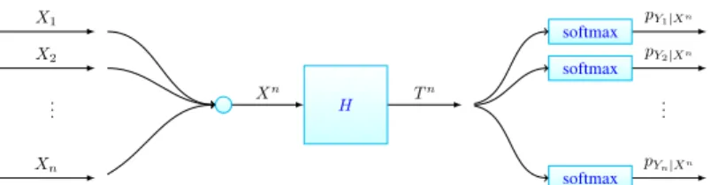
Briefly, in AgrLearn, a neural network classification model is structured to simultaneously classify n objects (Figure 1). This resembles a standard vector quantizer, which simultaneously quantizes multiple signals. In the training of the AgrLearn model, n random training objects are aggregated to a single amalgamated object and passed to the model. When using the trained model for prediction, the input to the model is also an aggregation of n objects, which can be all different or replicas of the object.
We conduct extensive experiments, applying AgrLearn to the current art of deep learning architec-tures for image and text classification. Experimental results suggest that AgrLearn brings significant gain in classification accuracy. Furthermore, with a heuristic smoothing, AgrLearn achieves an error rate of 2.45% on Cifar10, breaking the current record over this dataset.
In practice, AgrLearn can be easily integrated into existing neural network architectures with just addition of a few lines of code. Furthermore our experiments suggest that AgrLearn can dramat-ically reduce the required training examples (e.g., by 80% on Cifar10). This can be particularly advantageous for real-world learning problem with scarce labeled data.
2
The Aggregated Learning Framework
H Xn X1 X2 Xn .. . softmax softmax softmax .. . Tn pY1|Xn pY2|Xn pYn|Xn
Figure 1: The Aggregated Learning (AgrLearn) framework. The small circle denotes concatenation. 2.1 Information Bottleneck Learning
Throughout the paper, a random variable will be denoted by a capitalized letter, say, X, and a value it may take is denoted by its lower-case version, say, x. The distribution of a random variable is denoted by p subscripted by the random variable, for example, pX.
We consider a generic classification setting. We useX to denote the space of objects to be classified, where an object X distributes according to an unknown distribution pXonX . Let Y denote the space
of class labels. There is an unknown function F : X → Y which assigns an object X a class label Y := F (X). Let DX := {x1, x2, . . . , xN} be a given set of training examples, drawn i.i.d. from
pX. The objective of learning in this setting is to find an approximation of F based on the training
setD := {(xi, F(xi) : xi∈ DX}.
In the information bottleneck (IB) formulation [18] of such a learning problem, one is interested in learning a representation T of X in another spaceT . We will refer to T as a bottleneck representa-tion. When using a neural network model for classification, in this paper, we regard T as the vector computed at the final hidden layer of the network before it is passed to a standard soft-max layer to generate the predictive distribution overY. We will denote by h the function implemented by the network that computes T from the X, namely, h corresponds to the part of the network from input all the way to the final hidden layer and T = h(X).
The IB method insists the following fundamental principles. I. The mutual information I(X; T ) should be as small as possible. II. The mutual information I(Y ; T ) should be as large as possible.
Principle I insists that h squeeze out the maximum amount of information contained in X so that the information irrelevant to Y is removed from T . Principle II insists that T contain the maximum amount of information about Y so that all information relevant to classification is maintained. Intu-itively, the first principle forces the model not over-fitted to the irrelevant features of X, whereas the second aims at maximizing the classification accuracy.
In general the two principles have conflicting objectives. A natural approach to deal with this conflict is to set up a constrained optimization problem which implements one principle as the objective function and the other as the constraint. This results in the following problem formulations, where T is random variable taking values inT and forming a Markov chain Y − X − T with (Y, X).
b
pT|X := arg min pT|X:I(Y ;T )≥A
I(X; T ) for some prescribed value A (1) We refer to this problem as the IB learning problem and denote by RIB−learn(A) the minimum value
will adopt this assumption for now and later discuss the realistic setting in which one only has access to the empirical observation of pXY through training data.
It is worth noting that the IB learning problem in (1) is in fact more general than learning the bottleneck T in a neural network. This latter problem, which we refer to as the Neural Network IB
(NN-IB) learning problem, restricts that T depend on X deterministically, namely, having the form bh := arg min
h:I(Y ;T )≥AI(X; T ) (2)
The minimum value of the objective function in (2) will be denoted by RIB−NN(A).
The first observation we make in this paper is the following result.
Lemma 1 For any given pXY and bottleneck spaceT , RIB−learn(A) ≤ RIB−NN(A). Furthermore,
there exist pXY andT such that this inequality holds strictly.
This lemma suggests that using a neural network model for IB learning is in general not optimal. We will show later that AgrLearn presented in this paper may be seen as augmenting a standard network model to overcome its limitation.
The formulation of IB learning (1) resembles greatly the rate-distortion problem [15] in information theory, which studies the fundamental limit of quantization. This observation, also made in [11], in fact has motivated the approach of this paper.
We next introduce a special kind of quantization problem and show its connection to IB learning.
2.2 The IB Quantization Problem
Suppose that the distribution pXunder pXY characterizes an information source, which generates
a sequence of i.i.d. random variables(X1, X2, . . . , Xn). Throughout the paper, any sequence of
random variables(X1, X2, . . . , Xn), i.i.d. or not, will also be denoted by Xn.
Given pXY and the bottleneck space T , an (n, 2nR) IB-quantization code is a pair (fn, gn) of
functions, in which fn : Xn → {1, 2, . . . , 2nR} maps each sequence in Xn to an integer in
{1, 2, . . . , 2nR} and g
n : {1, 2, . . . , 2nR} → Tnmaps an integer in{1, 2, . . . , 2nR} to a sequence
inTn
. Using this code, fnencodes the sequence Xnas the integer fn(Xn), and gn“reconstructs”
Xnas a representation g
n(fn(Xn)) in Tn. The quantity R is referred to as the rate of the code.
Given pXY andT , let the distortion dIB(x, t; qY|X, qY|T) between any x ∈ X and any t ∈ T with
respect to any two arbitrary conditional distributions qY|X and qY|T be defined by
dIB(x, t; qY|X, qY|T) := KL(qY|X(·|x)||qY|T(·|t)), (3)
where qY|T(y|t) := P x∈X
qX|T(x|t)qY|X(y|x), and KL(·||·) denotes the KL divergence.
Given pXY, the code (fn, gn) induces a joint distribution pYnXnTn between the i.i.d. pairs (Y1, X1), (Y2, X2), . . . , (Yn, Xn) and Tn := (T1, T2, . . . , Tn) := gn(fn(Xn)). Under this
joint distribution, the distributions pYi,Xi,Ti, pYi|Xi, and pYi|Ti are all well defined for each i = 1, 2, . . . , n. Then for every two sequences xn ∈ Xn
and tn ∈ Tn
, define their IB
distor-tionas dIB(xn, tn) := 1 n n X i=1 dIB(xi, ti; pYi|Xi, pYi|Ti).
Under these definitions, the IB quantization problem is to find an IB-quantization code(fn, gn)
having the smallest rate R subject to constraint EdIB(Xn, Tn) ≤ D, where E denotes
expecta-tion. Note that different from the distortion function in a conventional quantization problem, the IB distortion function dIBin fact depends on the choice of IB-quantization code(fn, gn).
Before presenting the rate-distortion results for IB quantization, we relate an IB-quantization code to the bottleneck-generating function h in the neural network.
Lemma 2 The function h in the neural network is equivalent to a (1, 2R) IB-quantization code
In the language of quantization, an(f1, g1) quantization code is referred to as a scalar quantizer,
which encodes and reconstructs the signal X one at a time; an(fn, gn) quantization code with
n > 1 is referred to as a vector quantizer, which encodes and reconstructs n signals all together. Using these terminologies, the conventional neural network models are “scalar quantizers”, since they classify objects one at a time.
With conventional quantization problem, it is well known that vector quantizers can provide higher
efficiencyin terms of achieving the same level of distortion at a lower rate. We next show that this is also the case for the IB quantization problem.
Given pXY andT , a rate distortion pair (R, D) is said to be n-achievable if there exists an (n, 2nR)
IB-quantization code(fn, gn) such that EdIB(Xn, Tn) ≤ D. The pair (R, D) is said to be
∞-achievable, or simply, achievable, if there exists a sequence of (n, 2nR) IB-quantization codes
(fn, gn) such that lim
n→∞EdIB(X
n, Tn) ≤ D.
Lemma 3 Let m be a positive integer. For any given pXY andT , if a rate-distortion pair (R, D) is
m-achievable, then(R, D) is also km-achievable for any integer k > 1.
By this lemma, for any scalar quantizers(f1, g1), there is a vector quantizer that is at least as efficient.
Given pXY andT , the IB rate-distortion function RIB−RD(D) is the infimum of all rates R for
which(R, D) is achievable.
Theorem 1 Given pXY andT , the IB rate-distortion function is
RIB−RD(D) = min
pT|X:EdIB(X;T )≤D
I(X; T ) (4)
where the expectation is over the Markov chain Y − X − T specified by pXY and pT|X.
We note that a similar result to this theorem is also proved in [11]. However, in [11], the result (Theorem 2 therein) relies on a strong assumption on the cardinalities ofX and T , which is not required in the above theorem.
Lemma 4 There exist some pXY andT such that some rate-distortion pair (R, D) satisfying R =
RIB−RD(D) is not 1-achievable.
That is, achieving the fundamental limit RIB−RD(D) for IB quantization in general requires vector
quantizers. In fact, in many cases, the limit is only achievable at asymptotically large n.
2.3 IB Learning as IB Quantization
Theorem 2 RIB−learn(A) = RIB−RD(I(X; Y ) − A).
This theorem suggests that solving the IB learning problem that achieves RIB−learn(A) is equivalent
to finding the optimal IB-quantization code that achieves RIB−RD(I(X; Y ) − A) (noting that given
pXY, I(X; Y ) is merely a given constant). But as suggested in Lemma 1, the standard neural
network model in general cannot provide the optimal pT|X, paralleling the fact suggested in Lemma
4 that scalar IB quantizer is not optimal. On the other hand, as indicated in Theorem 1, there always exist vector quantizers (having possibly infinitely large n) which are optimal. This calls for a neural network learning approach that corresponds to vector IB quantizers.
2.4 Aggregated Learning (AgrLearn)
Based on the above analysis, we now present the framework of Aggregated Learning, or AgrLearn in short, for neural networks.
Instead of taking a single object inX as input, AgrLearn takes n objects Xn
as input. Here the value n is prescribed by the model designer and is referred to as the fold of AgrLearn. In fold-n AgrLearn (Figure 1), the bottleneck is generated as Tn= H(Xn) using some function H, and this “aggregated
bottleneck” Tnis then passed to n parallel soft-max layers. Let softmax(y
i|H(xn); θi) denote the
ithsoftmax layer, with learnable parameter θi, which maps the bottleneck H(xn) to the predictive
distribution pYi|Xnof label Yi. The AgrLearn model then states
pYn|Xn(yn|xn) = n Y i=1 pYi|Xn(yi|x n) = n Y i=1 softmax(yi|H(xn); θi). (5)
We note that (5) may appear to contradict the usual understanding that(Xi, Yi)’s are independent.
To clear any doubts about this, we remark that this understanding of independence is not incorrect. However, as suggested in Lemma 1, neural network models that implement this independence can be inadequate to provide the optimal bottleneck representation under the IB learning principle. This “contradiction” in question resembles the fact in the conventional quantization that even when the source signals are independent, it is still beneficial to quantize them jointly [2].
To train the AgrLearn model, a number of aggregated training examples are formed (as many as one can), each by concatenating n random objects sampled fromDX with replacement. We then
minimize the cross-entropy loss over all aggregated training examples.
When using the trained model for prediction, the following “Replicated Classification” protocol is used1. Each object X is replicated n times and concatenated to form the input. The average of n predictive distributions generated by the model is taken as the label predictive distribution for X.
2.5 Complication of Finite Sample Size N
The analysis above that motivates AgrLearn is based on the assumption that pXY is known. This
assumption corresponds to the asymptotic limit of infinite number N of training examples. In such a limit and assuming sufficient capacity of AgrLearn, larger aggregation fold n in theory gives rise to better bottleneck T (in the sense of minimizing I(X; T ) subject to the I(Y ; T ) constraint). In practice, one however only has access to the empirical distributionpeXY through observing the N
training examples inDX. As such, AgrLearn, in the large-n limit, can only solve for the empirical
version of the optimization problem (1), namely, findingminpT
|X:eI(Y ;T )≥AI(X; T ), where ee I(X; T ) and eI(Y ; T ) are I(X; T ) and I(Y ; T ) induced by epXY and pT|X. The solution to the empirical
version of the problem in general deviates from that to the original problem. Thus we expect, for finite N , that there is a critical value n∗of fold n, above which AgrLearn degrades its performance with increasing n. How to characterize n∗remains open at this time. Nonetheless it is sensible to expect that n∗increases with N , since larger N makespe
XY better approximate pXY.
With finite N , the product(epXY) n
of the empirical distributionepXY is a non-smooth
approxima-tion of the true product(pXY)n, and the “non-smoothness” increases with n. Intuitively, instead
of using(epXY) n
to approximate(pXY) n
, using some smoother approximations may improve the performance of AgrLearn. In some of our experiments, we incorporate the strategy of “MixUp”[24] as a heuristics to smooth(epXY)nin AgrLearn.
3
Experimental Studies
We evaluate AgrLearn with several widely deployed deep network architectures for classification tasks in the image and natural language domains. Standard benchmarking data sets are used. Unless otherwise specified, fold number n= 8 is used in all AgrLearn models.
All models examined are trained using mini-batched backprop for 400 epochs2 with exactly the
samehyper-parameter settings without dropout. Specifically, weight decay is10−4, and each
mini-batch contains 64 aggregated training examples. The learning rate is set to 0.1 initially and decays by a factor of 10 after 100, 150, and 250 epochs for all models. Each reported performance value (accuracy or error rate) is the median of the performance values obtained in the final 10 epochs.
1
Two additional protocols are in fact also investigated. Contextual Classification: For each object X, n− 1
random examples are drawn fromDX and concatenated with X to form the input; the predictive distribution
for X generated by the model is then retrieved. Repeat this process k times, and take the average of the k
predictive distribution as the label predictive distribution for X. Batched Classification: LetDtest
X denote the
set of all objects to be classified. In Batched Classification,Dtest
X are classified jointly through drawing k
random batches of n objects fromDtest
X . The objects in the i
th
batch Biare concatenated to form an input and
passed to the model. The final label predictive distribution for each object X inDtest
X is taken as the average
of the predictive distributions of X output by the model for all batches Bi’s containing X. Since we observe
that all three protocols result in comparable performances, all results reported in the paper are obtained using the Replicated Classification protocol.
2
3.1 Image Recognition
Experiments are conducted on the Cifar10 and Cifar100 datasets, both having 50,000 training images and 10,000 test images. The former contains 10 image classes and the latter contains 100. We apply AgrLearn to the 18-layer Pre-activation ResNet (“ResNet-18”) [3] implemented in [8]. The resulting AgrLearn model (“AgrLearn-ResNet-18”) differs from ResNet-18 only in its n parallel soft-max layers (as opposed to the single soft-max layer in ResNet-18).
Predictive Performance The prediction error rates of AgrLearn-ResNet-18 and ResNet-18 are shown in Table 1. It can be seen that AgrLearn significantly boosts the performance of ResNet-18,
Dataset ResNet-18 AgrLearn-ResNet-18 Relative Improvement over ResNet-18
Cifar10 5.53 4.73 14.4%
Cifar100 25.6 23.7 7.4%
Table 1: Test error rate (%) comparison of AgrLearn-ResNet-18 and ResNet-18
with relative error reductions of 14.4% and 7.4% on Cifar10 and Cifar100 respectively. Remarkably this performance gain simply involves plugging an existing neural network architecture in AgrLearn without any (hyper-)parameter tuning.
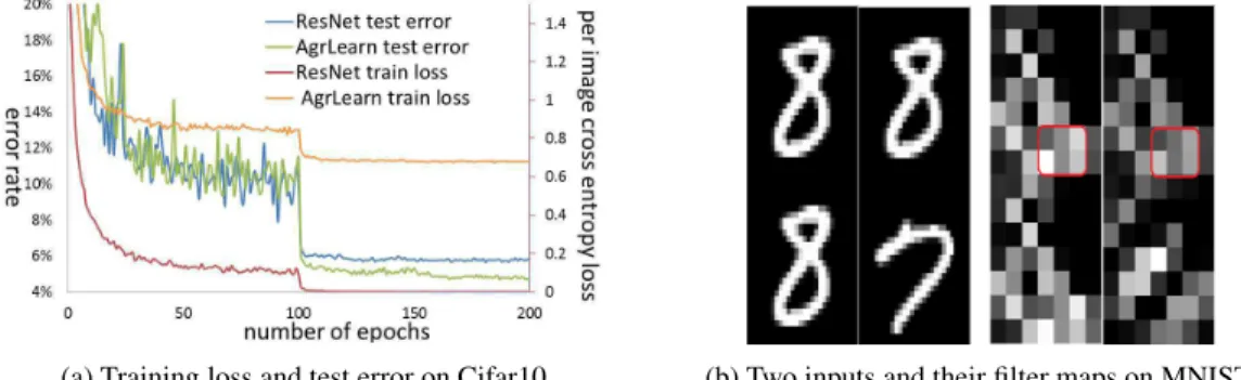
Model Behavior During Training The typical behavior of AgrLearn-ResNet-18 and ResNet-18 (in terms of training cross-entropy loss and testing error rate) across training epochs is shown in Fig-ure 2a. It is seen that during earlier training epochs, the test error of Agrlearn (green curve) fluctuates more than that of ResNet (blue curve) until both curves drop and stabilize. In the “stable phase” of training, the test error of AgrLearn continues to decrease whereas the test performance of ResNet cannot be further improved. This can be explained by the training loss curve of ResNet (red curve), which drops to zero quickly in this phase and provides no training signal for further tuning the net-work parameters. In contrast, the training curve of AgrLearn (brown curve) maintains a relatively high level, allowing the model to keep tuning itself. The relatively higher training loss of AgrLearn is due to the much larger space of the amalgamated examples. Even in the stable phase, one expects that the model is still seeing new combinations of images. In a sense, we argue that aggregating several examples into a single input can be seen as an implicit form of regularization, preventing the model from over-fitted by individual examples.
(a) Training loss and test error on Cifar10. (b) Two inputs and their filter maps on MNIST.
Figure 2: Training/testing curves and filter maps visualization.
Feature Map Visualization To visualize the extracted feature by AgrLearn, we perform a small experiment on MNIST using a fold-2 AgrLearn on a 3-layer CNN as implemented in [20]. Here we consider a binary classification task where only images for digits “7” and “8” are to be classified. Figure 2b shows two amalgamated input images (left two) and their corresponding feature maps obtained at the final hidden layer of the learned model. Note that the top images in the two inputs are identical, but since they are paired with different images to form the input, different features are extracted (e.g., the regions enclosed by the red boxes). This confirms that AgrLearn extracts joint features across the aggregated examples, as we expect in our design rationale for AgrLearn. Sensitivity to Model Complexity With fold-n AgrLearn, the output label space becomesYn
. This significantly larger label space seems to suggest that AgrLearn favors more complex model. In this study, we start with AgrLearn-ResNet-18 and investigate the behavior of the model when it becomes more complex. The options we investigate include increasing the model width (by doubling or
tripling the number of filters per layer) and increasing the model depth (from 18 layers to 34 layers). The performances of these models are given in Table 2.
Table 2 shows that increasing the model width improves the performance of AgrLearn on both Cifar10 and Cifar100. For example, doubling the number of filters reduces the error rate from 4.73% to 4.2% on Cifar10, and tripling it further decreases the error rate to 4.14%.
Data set 18 layers 18 layers+double 18 layers+triple 34 layers 34 layers+double
Cifar10 4.73 4.20 4.14 5.01 4.18
Cifar100 23.70 21.18 20.21 22.18 22.02 Table 2: Test error rates (%) of AgrLearn-ResNet-18 (“18 layer”) and its more complex variants
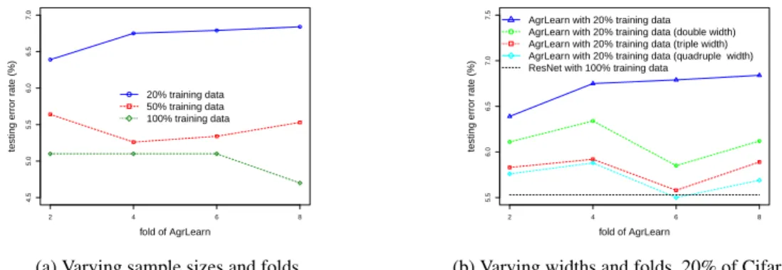
However increasing the model depth is not as effective. For example, on Cifar10, AgrLearn-ResNet-18 (with error rate 4.73%) outperforms its 34-layer variant (error rate of 5.01%). But the 34-layer model, when further enhanced by the width, has a performance boost (to error rate 4.18%). On Cifar100, increasing AgrLearn-ResNet-18 to 34 layers only slightly improves its performance. We hypothesize that with AgrLearn, the width of a model plays a critical role. This is because the model must extract joint features across individual objects in the amalgamated example. Nonethe-less optimizing over width and optimizing over depth are likely coupled, and they may be further complicated by the internal computations in the model, such as convolution, activation, and pooling. Behavior with Respect to Fold Number and Robustness to Data Scarcity We also conduct ex-periments investigating the performance of AgrLearn-ResNet-18 with varying fold n and with re-spect to varying training sample size N . The Cifar10 dataset is used in this study, as well as two of its randomly reduced subsets, one containing 20% of the training data and the other containing 50%. Figure 3a suggests that the performance of AgrLearn models vary with fold n. The best performing fold number for AgrLearn-ResNet-18 on 20%, 50% and 100% of the Cifar10 dataset appears to be 2, 4, and 8 (or larger) respectively. This supports our conjecture in Section 2.5 regarding the existence of the critical fold n∗.
Using only 20% of Cifar10, we investigate the performance of AgrLearn-ResNet-18 with increasing widths, namely, with the number of filters doubled, tripled, or quadrupled. In Figure 3b we see that the fold-6 triple-width and quadruple-width AgrLearn-ResNet-18 models trained using 20% of Cifar10 perform comparably to or even better than ResNet-18 trained on the entire Cifar10. This demonstrates the robustness of AgrLearn to data scarcity, making AgrLearn an appealing solution to practical learning problems with inadequate labeled data.
4.5 5.0 5.5 6.0 6.5 7.0 2 4 6 8 fold of AgrLearn testing error r ate (%) 20% training data 50% training data 100% training data
(a) Varying sample sizes and folds
5.5 6.0 6.5 7.0 7.5 2 4 6 8 fold of AgrLearn testing error r ate (%)
AgrLearn with 20% training data AgrLearn with 20% training data (double width) AgrLearn with 20% training data (triple width) AgrLearn with 20% training data (quadruple width) ResNet with 100% training data
(b) Varying widths and folds, 20% of Cifar10
Figure 3: Performances of AgrLearn-ResNet-18 and its variants on Cifar10 and its reduced datasets
New State Of The Art Following the discussion in Section 2.5, we apply a recent data augmentation method MixUp [24] as a heuristics to smooth(epXY)
n
. Briefly, MixUp augments the training data with synthetic training examples, each obtained by interpolating a pair of original examples and their corresponding labels. In our experiments, we apply this strategy to triple-width AgrLearn-ResNet-18, where the ResNet structure follows that in [8]. Specifically, MixUp is deployed to the 8-fold amalgamated images and their label vectors to augment the training set. This model turns out to achieve an error rate of 2.56% on Cifar10, beating the current best record of 2.7%,
reported in [24]. Note that the current best record was achieved by a WideResNet architecture [22] of 28 layers, also augmented with MixUp. We then apply AgrLearn to the same WideResNet architecture as implemented in [21] but only using 22 layers. When augmented with MixUp, this model gives rise to an even lower error rate of 2.54%. At this end, we have provided two new state-of-the-art performance records, by simply applying AgrLearn to existing models and augmenting the amalgamated data with MixUp. These results, to an extent validating our analysis in Section 2.5, are summarized in Table 3.
Dataset Reported SOTA AgrLearn AgrLearn Cifar10 2.7% (WideResNet-28-10/MixUp) 2.56% (ResNet-18) 2.45% (WideResNet-22)
Table 3: Error rates (%): new state of the art (SOTA) established by AgrLearn.
3.2 Text Classification
We test AgrLearn with two widely adopted NLP deep-learning architectures, CNN and LSTM [4], using two benchmark sentence-classification datasets, Movie Review [13]3 and Subjectivity [12].
Movie Review and Subjectivity contain respectively 10,662 and 1,000 sentences, with binary labels. We use 10% of random examples in each dataset for testing and the rest for training, as is in [5]. For CNN, we adopt CNN-sentence [5] and implement it exactly as in [6]. For LSTM, we just simply replace the convolution and pooling components in CNN-sentence with standard LSTM units as implemented in [1]. The final feature map of CNN and final state of LSTM are passed to a logistic regression classifier for label prediction. Each sentence enters the models via a learnable, randomly initialized word-embedding dictionary. For CNN, all sentences are zero-padded to the same length. The fold-2 AgrLearn models corresponding to the CNN and LSTM models are also constructed. In AgrLearn-CNN, the aggregation of two sentences in each input simply involves concatenating the two zero-padded sentences. In AgrLearn-LSTM, when two sentences are concatenated in tandem, an EOS word is inserted after the first sentence.
We train and test the CNN, LSTM and their respective AgrLearn models on the two datasets, and report their performances in Table 4. Clearly, the AgrLearn models improve upon their correspond-ing CNN or LSTM counterparts. In particular, the relative performance gain brought by AgrLearn on the CNN model appears more significant, amounting to 4.2% on Movie Review and 3.8% on Subjectivity.
Dataset CNN AgrLearn-CNN LSTM AgrLearn-LSTM Movie Review 76.1 79.3 76.2 77.8 Subjectivity 90.01 93.5 90.2 92.1
Table 4: Accuracy (%) obtained by CNN, LSTM and their respective AgrLearn models.
4
Conclusion, Discussion and Outlook
Aggregated Learning, or AgrLearn, is a simple and effective neural network modeling framework, justified information-theoretically. It builds on a connection between IB learning and IB quantiza-tion and exploits the power of vector quantizaquantiza-tion. As shown in our experiments, it can be applied to an existing network architecture with virtually no programming or tuning effort. We have demon-strated its effectiveness through the significant performance gain it brings to the current art of deep network models and through the two new state-of-the-art classification accuracies that we have eas-ily obtained. Its robustness to small training sample is also a salient feature, making AgrLearn particularly attractive in practice, where the labeled data may not be abundant.
We need to acknowledge that the gain brought by AgrLearn is not free of cost. In fact, the memory consumption of fold-n AgrLearn is n times what is required by the conventional model.
Simultaneously classifying several examples, AgrLearn is reminiscent of “collective inference” [9, 10], a setting in which several correlated random variables are inferred all at once. Although the two settings also exhibit adequate differences in methodologies and principles, it is perhaps interesting to investigate if there is a deeper connection between the two.
3
Another line of research, seemingly related to AgrLearn, is data augmentation [17, 19, 24], in-cluding, for example, MixUp. In our opinion, however, it is incorrect to regard AgrLearn as a data augmentation scheme. Aggregating examples in AgrLearn expands the input space, which induces additional modeling freedom (although we made little effort in this work exploiting this freedom). Such a property, not possessed by data augmentation schemes, clearly distinguishes AgrLearn from those schemes.
The motivation of AgrLearn is the fundamental notion of information bottleneck (IB). The effec-tiveness of AgrLearn demonstrated in this paper may serve as additional validation of the IB theory. The proposal and successful application of AgrLearn in this paper are believed to signal the begin-ning of a rich theme of research. Interesting questions may include: how can we characterize the interaction between model complexity, fold number and sample size in AgrLearn? and how can we fully exploit the modeling freedom in AgrLearn?
References
[1] M. Abadi, P. Barham, J. Chen, Z. Chen, A. Davis, J. Dean, M. Devin, S. Ghemawat, G. Irving, M. Isard, M. Kudlur, J. Levenberg, R. Monga, S. Moore, D. G. Murray, B. Steiner, P. Tucker, V. Vasudevan, P. Warden, M. Wicke, Y. Yu, and X. Zheng. Tensorflow: A system for large-scale machine learning. In Proceedings of the 12th USENIX Conference on Operating Systems
Design and Implementation, OSDI’16, pages 265–283, 2016.
[2] T. M. Cover and J. A. Thomas. Elements of Information Theory (Wiley Series in
Telecommu-nications and Signal Processing). Wiley-Interscience, New York, NY, USA, 2006.
[3] K. He, X. Zhang, S. Ren, and J. Sun. Identity mappings in deep residual networks. In Computer
Vision - ECCV 2016, Part IV, pages 630–645, 2016.
[4] S. Hochreiter and J. Schmidhuber. Long short-term memory. Neural Comput., 9(8):1735– 1780, Nov. 1997.
[5] Y. Kim. Convolutional neural networks for sentence classification. In EMNLP, pages 1746– 1751, 2014.
[6] Y. Kim. https://github.com/yoonkim/cnn sentence, 2014.
[7] Y. LeCun, Y. Bengio, and G. E. Hinton. Deep learning. Nature, 521(7553):436–444, 2015.
[8] K. Liu. https://github.com/kuangliu/pytorch-cifar, 2017.
[9] S. A. Macskassy and F. Provost. Classification in networked data: A toolkit and a univariate case study. J. Mach. Learn. Res., 8:935–983, May 2007.
[10] J. Moore and J. Neville. Deep collective inference. In AAAI, pages 2364–2372, 2017.
[11] R. G.-B. A. Navot and N. Tishby. An information theoretic tradeoff between complexity and accuracy. In COLT, 2003.
[12] B. Pang and L. Lee. A sentimental education: Sentiment analysis using subjectivity summa-rization based on minimum cuts. In ACL, pages 271–278, 2004.
[13] B. Pang and L. Lee. Seeing stars: Exploiting class relationships for sentiment categorization with respect to rating scales. In ACL, pages 115–124, 2005.
[14] O. Shamir, S. Sabato, and N. Tishby. Learning and generalization with the information bottle-neck. Theor. Comput. Sci., 411(29-30):2696–2711, June 2010.
[15] C. E. Shannon. Coding theorems for a discrete source with a fidelity criterion. IRE National
Convention Record, 7, 1959.
[16] R. Shwartz-Ziv and N. Tishby. Opening the black box of deep neural networks via information.
CoRR, abs/1703.00810, 2017.
[17] P. Y. Simard, Y. A. L. Cun, J. S. Denker, and B. Victorri. Transformation invariance in pattern recognition - tangent distance and tangent propagation. In Neural Networks: Tricks of the
Trade, This Book is an Outgrowth of a 1996 NIPS Workshop, pages 239–274. Springer, 1998. [18] N. Tishby, F. C. Pereira, and W. Bialek. The information bottleneck method. In Proceedings of
37th Annual Allerton Conference on Communication, Control and Computing, pages 368–377, 1999.
[19] V. Verma, A. Lamb, C. Beckham, A. C. Courville, I. Mitliagkas, and Y. Bengio. Man-ifold mixup: Encouraging meaningful on-manMan-ifold interpolation as a regularizer. CoRR, abs/1806.05236, 2018.
[20] Y. Wu et al. Tensorpack. https://github.com/tensorpack/, 2016.
[21] S. Zagoruyko and N. Komodakis. https://github.com/szagoruyko/ wide-residual-networks, 2016.
[22] S. Zagoruyko and N. Komodakis. Wide residual networks. In Proceedings of the British
Machine Vision Conference 2016, BMVC 2016, York, UK, September 19-22, 2016, 2016. [23] C. Zhang, S. Bengio, M. Hardt, B. Recht, and O. Vinyals. Understanding deep learning requires
rethinking generalization. ICLR, 2017.
[24] H. Zhang, M. Ciss´e, Y. N. Dauphin, and D. Lopez-Paz. mixup: Beyond empirical risk mini-mization. In ICLR, 2017.