HAL Id: halshs-00768434
https://halshs.archives-ouvertes.fr/halshs-00768434
Preprint submitted on 21 Dec 2012HAL is a multi-disciplinary open access archive for the deposit and dissemination of sci-entific research documents, whether they are pub-lished or not. The documents may come from teaching and research institutions in France or abroad, or from public or private research centers.
L’archive ouverte pluridisciplinaire HAL, est destinée au dépôt et à la diffusion de documents scientifiques de niveau recherche, publiés ou non, émanant des établissements d’enseignement et de recherche français ou étrangers, des laboratoires publics ou privés.
Bubbles and Incentives : An Experiment on Asset
Markets
Stéphane Robin, Katerina Straznicka, Marie Claire Villeval
To cite this version:
Stéphane Robin, Katerina Straznicka, Marie Claire Villeval. Bubbles and Incentives : An Experiment on Asset Markets. 2012. �halshs-00768434�
GROUPE D’ANALYSE ET DE THÉORIE ÉCONOMIQUE LYON -‐ ST ÉTIENNE W P 1235
Bubbles and Incentives: An Experiment on Asset Markets
Stéphane Robin, Katerina Straznicka, Marie Claire Villeval December 2012
Doc
ume
nt
s
de
tr
av
ai
l |
W
or
ki
ng
P
ape
rs
GATE Groupe d’Analyse et de Théorie Économique Lyon-‐St Étienne
93, chemin des Mouilles 69130 Ecully – France Tel. +33 (0)4 72 86 60 60
Fax +33 (0)4 72 86 60 90
6, rue Basse des Rives 42023 Saint-‐Etienne cedex 02 – France Tel. +33 (0)4 77 42 19 60
Fax. +33 (0)4 77 42 19 50
Messagerie électronique / Email : [email protected]
Téléchargement / Download : http://www.gate.cnrs.fr – Publications / Working Papers
Bubbles and Incentives: An Experiment on Asset Markets
Stéphane ROBINa, Kateřina STRAZNICKAa and Marie Claire VILLEVALab
Abstract: We explore the effects of competitive incentives and of their time horizon on the
evolution of both asset prices and trading activity in experimental asset markets. We compare
i) a no-bonus treatment based on Smith, Suchanek and Williams (1988); ii) a short-term bonus
treatment in which bonuses are assigned to the best performers at the end of each trading period; iii) a long-term bonus treatment in which bonuses are assigned to the best performers at the end of the 15 periods of the market. We find that the existence of bonus contracts does not increase the likelihood of bubbles but it affects their severity, depending on the time horizon of bonuses. Markets with long-term bonus contracts experience lower price deviations and a lower turnover of assets than markets with either no bonuses or long-term bonus contracts. Short-term bonus contracts increase price deviations but only when markets include a higher share of male traders. At the individual level, the introduction of bonus contracts increases the trading activity of males, probably due to their higher competitiveness. Finally, both mispricing and asset turnover are lower when the pool of traders is more risk-averse.
Keywords: Asset market, bubbles, incentives, bonuses, risk attitudes, experiment. JEL codes: C92, M52
a University of Lyon, Lyon, 69007, France ; CNRS, GATE Lyon Saint-Etienne, Ecully,
F-69130, France. E-Mail: [email protected], [email protected], [email protected].
b IZA, Bonn, Germany.
We are thankful for helpful suggestions to participants at the 4th EWEBE workshop in
Barcelona, the 1st SEBA-GATE workshop in Beijing, the CIRPEE workshop on Advances in
Experimental Economics at the University of Paris I, the INAPOR Workshop in Nice, and at a seminar at the University of Bern. We are also grateful to S. Cheung and C. Noussair for comments on a previous version of this paper. We thank V. Lei for providing us the computer software used in this experiment and V. Verdier for helpful research assistance. Financial support from Agence Nationale de la Recherche (ANR BLAN07-3_185547, EMIR project) is gratefully acknowledged.
2
Bubbles and Incentives: An Experiment on Asset Markets
1. INTRODUCTION
Financial bubbles in asset markets - defined as ‘trade in high volume at prices that are considerably at variance from intrinsic value’ (King et al., 1993) - have serious consequences for the economy as a whole. Mispricing generates severe distortions in the allocation of capital and bubble crashes destroy a large amount of wealth and have adverse repercussions for the wider economy, as illustrated by the current global financial crisis. This phenomenon is in contrast with the efficient market hypothesis where actual prices reflect the asset’s fundamental value (Fama, 1970). Indeed, if traders share the same priors about an asset’s value, there should be no gain to trade (Tirole, 1982).1 Speculation then relies on inconsistent plans and should be ruled out by rational expectations. Recently, the responsibility of traders’ compensation schemes has been pointed out as a potential cause of speculation and increased volatility of stock markets. Traders are often perceived as trading at excessively high frequency and as taking excessive risks in the markets in the pursuit of ever-greater bonuses. In particular, the Pittsburgh meeting of the Group of twenty finance ministers and central bank governors in September 2009 has insisted on the importance of reforming traders’ compensation practices in order to support financial stability (G20 Leaders, 2009).2
1 The no-trade theorem states that when rational and risk-neutral traders participate in a market with ex ante
Pareto-optimal allocation and receive private information, they can still never agree to any trade (Milgrom and Stokey, 1982).
2 Its final declaration stated: “Excessive compensation in the financial sector has both reflected and encouraged
3
The main aim of this paper is to study whether traders’ competitive incentives contribute to the emergence and the severity of bubbles in asset markets. We analyze whether the introduction of competitive bonus contracts in traders’ compensation packages influences the occurrence of bubbles and crashes. We manipulate the time-horizon of the bonuses and the portfolio valuation in their calculation to measure their influence on the efficiency of asset markets. Precisely, we test whether mispricing is increased by the distribution in each period of short-term bonuses for which portfolios are valued at the current market price. And we test whether it is decreased by the payment of long-term bonuses at the end of the market when portfolios are valued at their fundamental value.
Since individual survey data on traders’ compensation schemes are not easily accessible, we privilege here an experimental approach. This allows us to relate potential deviations from the assets’ fundamental value to the introduction of various types of bonuses in traders’ compensation schemes. To the best of our knowledge, only three studies have considered the effect of compensation schemes on mispricing in experimental asset markets. These studies are based on the multi-periods asset-life markets experimental design introduced in Smith, Suchamek and Williams (1988). James and Isaac (2000) and Isaac and James (2003) introduce tournaments whose winners are determined at the end of the last trading period. They find that “beating-the-market” incentives increase mispricing. In contrast with their design, in our experiment market prices are a component of the performance measure that conditions the assignment of bonuses. Cheung and Coleman (2011) show that league-table incentives that are paid each four periods on the basis of the recent growth in the value of the traders’ portfolio
financial stability. We fully endorse the implementation standards of the FSB aimed at aligning compensation with long-term value creation, not excessive risk-taking…" (G20 Leaders, 2009)
4
amplify the price deviations above the intrinsic value of the assets. This effect increases with traders’ experience and is stronger when the fundamental value of assets is declining over time than in a constant-value environment. In contrast with these studies, we manipulate the frequency at which bonuses are distributed and we conduct our analysis both at the market and at the individual levels to better understand traders’ behavior in reaction to incentives. In particular, we study the role played by traders’ risk preferences on the dynamics of prices. Precisely, our design consists of three treatments of an asset market game. The baseline treatment (“no-bonus treatment”) mostly replicates the design of Smith, Suchanek and Williams (1988) (SSW, hereafter). Eight agents are endowed with an equal initial endowment in cash and shares and they can trade assets in a 15-periods asset-life market. Assets pay the same dividend to each trader in each period and the dividend is the only source of intrinsic value. The structure of dividends and the evolution of the fundamental value of the asset are common knowledge from the very beginning of the game. In contrast with the predictions of the no-trade theorem, the previous experimental literature has shown that trading is important in these markets. Prices typically diverge from the fundamental value of the assets, starting below the fundamental value and quickly rising above it until a crash occurs.3
3 Since the seminal work of SSW, numerous treatment manipulations of the original design have been tested: see
Palan, (2009) for a survey; King et al. (1993) on the influence of experience; Lei et al. (2001) on non-speculative bubbles; Noussair et al. (2001) on assets with constant fundamental values; Haruvy and Noussair (2006) on the effect of short-selling on mispricing; Oechssler et al. (2011) and Sutter et al. (2012) on the role of information; Cheung and Palan (2012) on the improvement permitted by team decision-making. Mispricing is robust to most of these manipulations, except an increased experience within the same group of traders, suggesting a responsibility of the lack of common expectations in bubble formation (see for instance Van Boening et al., 1993, or more recently on the same topics Cheung et al., 2012).
5
In order to measure how these results are affected by the nature of incentives, our two other treatments introduce bonus contracts. In the short-term bonus treatment, the top three performers receive in each period a bonus whose value depends on the traders’ performance rank. In the long-term bonus treatment, bonuses are awarded to the top three performers as measured after the 15 market periods have been completed. In the short-term bonus treatment, the trader’s performance is based on his or her profit in the current period and on the change of his or her portfolio’s value between the previous and the current period assessed at the current period average market price. In the long-term bonus treatment, the traders’ performance is assessed on the basis of the profits obtained over the life of the market. This manipulation allows us to test how different types of incentives influence market efficiency.
Our findings show that the introduction of bonus contracts does not increase the likelihood of bubbles in the asset markets but it affects their severity. The markets with long-term bonus contracts experience less price deviations, smaller bubble amplitude and less asset turnover than the markets with either short-term bonus contracts or no-bonus contracts. Moreover, mispricing is less severe and trade activity is less intense in markets with a higher share of risk-averse traders and of male traders. However, the impact of gender is reverted in the presence of short-term bonus contracts. Male traders react more to the introduction of competitive incentives in each period than female traders. Therefore, short-term bonus contracts are associated with significantly higher price deviations than the no-bonus contracts if the share of male traders increases. This is consistent with previous research showing that males are more attracted by competition (Niederle and Vesterlund, 2007; Villeval, 2012) and increase more effort in competitive environments than females (Gneezy, Niederle and Rustichini, 2003). Overall, our results reveal that the nature of incentives influences mispricing notably through a differentiated impact on the behavior of male traders.
6
The remainder of this paper is organized as follows. Section 2 surveys the related literature. Section 3 presents our experimental design, the procedures and our conjectures. Section 4 develops the experimental findings. Last, Section 5 discusses the results and concludes.
2. RELATED LITERATURE
Very few experimental studies have examined how competitive incentives affect the dynamics of asset markets.4 James and Isaac (2000) have provided the first test of the effect of tournament incentives on bubble formation, by means of a within-subject experiment based on the design of SSW (1988). In their experiment, nine traders participate in six successive 15 periods-life asset markets, with or without tournaments. The tournament is a ’beat-the-market’ incentive scheme: the traders who performed above average at the end of the 15 periods receive a bonus equal to twice the difference between their profit and the average profit; those who perform below average receive a flat payment. The results indicate that tournaments increase mispricing. In a follow-up study, Isaac and James (2003) show that when the proportion of traders with a tournament contract is reduced sufficiently, the impact of tournaments on mispricing disappears.
In contrast with this approach, we use a between-subject design to avoid the potential order effects of a within-subject design. In addition, at the end of the market traders earn the value of their cash balance and in one of our treatments, market prices are a component of the performance measure that conditions the assignment of bonuses. This is unlike the
4 This is also true in the field of personnel economics where the impact of tournament contracts has been studied
7
market’ principle used by James and Isaac. Another difference is that traders know the bonuses they can earn from the very beginning of the session.
Rather than paying a one-time bonus at the end of session, Cheung and Coleman (2011) introduce league-table incentives consisting of bonuses assigned at evenly-timed intervals over the life of the market on the basis of the ‘year-on-year’ growth in the paper value of the traders’ asset holdings. The three top-ranked traders receive an inflow amounting to double the payment they would have received in the baseline condition; the three middle-ranked traders receive an inflow amounting to the same payment as in the baseline condition; the last three traders receive nothing. Cheung and Coleman (2011) also study the influence of experience and they compare markets in which the fundamental value of the asset declines over time with markets in which the fundamental value is constant. They find that in the constant-value environment, the effect of incentives is mild; in contrast, in the declining-value environment, mispricing is greatly exacerbated by incentives. Even in experienced markets, prices climb to levels clearly indicative of speculation and bubbles do not always crash.
In contrast with this study, we manipulate the frequency at which bonuses are distributed to compare the impact of short-term versus long-term incentives. Moreover, we analyze our data not only at the market level but also at the individual level. In particular, we study the role played by traders’ risk preferences on their trading behavior and on the resulting dynamics of prices under the different incentive schemes.
The literature studying the influence of individual risk preferences on the efficiency of markets delivers contrasted results. On the one hand, Ang and Schwarz (1985) find that less risk-averse markets show greater price volatility but converge quicker to the equilibrium price. On the other hand, Fellner and Maciejovsky (2007) find that the higher the degree of risk aversion of traders, the lower the market activity. Last, Güth et al. (1997) find that in markets
8
with both informed and uninformed agents, risk attitudes do not explain portfolio structures. Our experiment should provide additional evidence on this relationship. As regards the impact of tournaments, Bronars (1986) has shown theoretically that risk-neutral agents allocate too much time to safe projects and that frontrunners limit risks while underdogs increase risk-taking in sequential tournaments. Risk-risk-taking may act as a substitute for effort (Hvide, 2002). Agents adopt high-risk-prospects when prizes and spread of prizes are high (e.g., Becker and Huselid, 1992; Gaba and Kalra, 1999; Lee, 2004), when only a top few win (Gaba and Kalra, 1999), and depending on the relative position in interim reports (e.g., Nieken and Sliwka, 2010). Studies in financial economics have also shown that relative performance objectives increase the riskiness of investment strategies (Palomino, 2005) and that investment fund managers paid on a yearly basis adjust the risk they take in the latter part of the year to their relative position mid-year. 5 Here, we test whether the impact of risk preferences on the dynamics of asset markets is influenced by the introduction of bonus contracts.
3. EXPERIMENTAL DESIGN, PROCEDURES, AND PREDICTIONS
Our between-subjects experiment consists of three treatments that are described successively. Then, we develop the procedures before introducing our behavioral conjectures.
5 There is, however, no consensus on which managers take riskier positions. Some find that those who increase
the fund volatility or portfolio risk more in the latter part of the year are the mid-year losers (e.g., Brown et al., 1996; Chevalier and Ellison, 1997; Kempf and Ruenzi, 2008); others find that interim winners are more likely to gamble since they expect that the underdogs will try to catch up (e.g., Busse, 2001; Qui, 2003; Taylor, 2003).
9
3.1. The treatments The no-bonus treatment
The no-bonus treatment replicates most aspects of the SSW’s (1988) procedure.6 It consists of a computerized continuous double auction market that allows eight participants to trade risky assets in real time in a sequence of 15 market periods. Each market period lasts 240 seconds. At the beginning of the experiment, each trader is given both an initial portfolio of 10 asset units and a cash endowment of 20,000 Experimental Currency Units (ECU, hereafter). The initial endowment of liquidity can be considered as a loan that has to be paid back at the end of the experiment.7 Trades follow continuous auction rules.8 Traders are allowed to trade one asset at a time and the order book has a depth of one (i.e., posted orders are automatically erased by better bids and asks). Short sells are not allowed. Traders can buy assets as long as their liquidity permits it; they are not granted credit. They all receive exactly the same initial endowments in shares and liquidity, and thus have identical ex ante earning opportunities. We do this to eliminate any possibility that the liquidity and asset unit composition of a trader’s initial endowment biases his or her position in the bonus contracts treatments.
6 There are three main differences with SSW (1988). First, we do not have traders that differ in the allocation of
shares and cash endowment. Second, we do not allow traders to bypass the stopping rule by voting to end a trading period before the maximum time has elapsed. Third, there is no rank queue for offers that do not improve the current posted offers. Further literature on experimental asset markets has shown that these differences do not alter the main conclusions of SSW (1988).
7 If a subject ends the game with a loss, this loss is deducted from her show-up fee and this is common
information. If the loss is higher than the show-up fee, we do not ask for any reimbursement. The market initial endowment in liquidity allows a trader to purchase more than 2/3 of the total stock of assets at the initial fundamental value. This large initial endowment was chosen in order not to constrain purchases in the market.
10
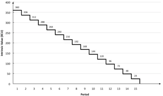
At the end of each period, each asset unit generates a stochastic dividend to its current owner. The actual dividend value is the same for all assets in the market and for everyone in a given period. The dividend payments are randomly drawn from a uniform distribution (0, 8, 28, 60 ECU). Therefore, the expected value of each asset is 24 ECU in each period. The earnings generated by dividend payments in each period are added to the owner’s liquidity at the end of the period. The dividend structure is common knowledge.
Assuming that traders are risk neutral and using backward induction, the asset’s fundamental value is equal to the expected total future flow of dividends. In any period, it is calculated as the number of dividend draws remaining until the end of the sequence of 15 periods times the expected dividend value (24 ECU). Thus, at the beginning of the sequence the fundamental value of each asset unit is 360 ECU (15*24), while it is only 24 ECU at the beginning of the fifteenth period. When the fifteenth period is over, the asset’s value equals zero. There is no buy-out option. Figure 1 displays the evolution of the asset’s fundamental value over time.
11
The dividend structure is made common information and precautions are taken to ensure that participants plainly understood this structure.9 The traders’ current liquidity and asset holdings are displayed on the screens and are automatically updated after each transaction and after each dividend payment. Once a period is over, traders receive summary information on the amount of the dividend payment drawn for this period, the total amount of asset holdings and liquidity. During a period, a history box displays all the transactions concluded in the market and their respective price since the beginning of the period.10
In a period, earnings are computed as the evolution of the liquidity during this period, i.e. the revenues generated by the stock sales minus the cost of stock purchases. They are augmented at the end of each trading period with the dividend earnings (the dividend value times the stock of asset holdings at the end of the period). Indeed, there are two sources of profits for the traders. The first one is related to both the trading activity and the evolution of stock prices. The other one consists of the dividend earnings. Therefore, the trader i’s profit in period t writes as follows:
Profitit = (stock sales revenuesit − stock purchase costsit)
+ (assetsit * dividendt) (1)
9 The calculation of the asset fundamental value is explained and exemplified in the instructions. Together with
the instructions participants receive a table indicating the fundamental value of each asset unit in each period. (see Appendix A).
10 At the end of a period, the participants have to record manually on an inventory and payoff table the evolution
of their liquidity during the current period, the number of asset units owned at the end of the period, the amount of the dividend, and the resulting earnings for the period. The reason we asked them to do so is to make them take into consideration the impact of their market behavior on the evaluation of their gains or losses.
12
The short-term bonus treatment
The short-term bonus treatment implements a rank-order tournament between the traders in each trading period. Precisely, at the end of each period the performance of the traders is compared. The three traders who realized the highest performance in the period earn a bonus on top of their profit of the period. Trader i’s performance in period t is calculated as follows:
Performanceit = Profitit + [(assetsit *average market pricet )
- (assetsi(t-1) *average market price(t-1) )] (2) The first term represents the trader’s profit as explained in equation (1). The second term captures the variation in the value of the trader’s portfolio between the end and the beginning of the current period calculated at the market price. The value of the trader’s portfolio at the beginning of a period equals the number of his or her asset holdings at the beginning of the period (namely the number of his asset holdings at the end of the previous period) multiplied by the average market price of all concluded transactions in the market during the previous period. The value of his or her portfolio at the end of the period equals the number of her asset holdings at the end of the period multiplied by the average market price of all concluded transactions within the current period. This representation of performance takes into account both the activity of the trader in the market and his or her ability to manage his or her capital in given short-term market conditions.11
In each period, the trader who realized the highest performance in the period receives a bonus of 240 ECU. The trader who realized the second highest performance receives a bonus of 168 ECU. The bonus of the trader who realized the third highest performance amounts to 72 ECU. The highest bonus corresponds to the expected dividend generated by 10 asset units during
11 In period 1, as there is no previous period of play, the performance accounts only for the portfolio development
13
one period. The second (third, respectively) bonus represents 70% (30%, resp.) of the value of the highest bonus. The bonus is added to the traders’ liquidity before the beginning of the next period. These amounts have been determined arbitrarily, such as to provide a salient additional incentive to realize a high performance without introducing too many additional liquidities in the market throughout the session.12
The long-term bonus treatment
The long-term bonus treatment also introduces a rank-order tournament between the traders but here, the traders’ performances throughout the session are compared at the end of the 15 periods. The three traders with the highest total performance earn a bonus which value depends on their rank. The best performer receives a bonus of 3,600 ECU, the second best performer receives a bonus of 2,520 ECU, and the third one a bonus of 1,080 ECU. The total amount of bonuses distributed is the same as in the short-term bonus treatment. Performance is measured as the sum of profits obtained during the 15 periods of the game. In contrast with the short-term bonus contracts, the portfolios are here valued at their fundamental value, as the current value of the asset holdings at the end of the market life is zero.
12 Indeed, this injection of liquidity could bias the comparison between the short-term bonus treatment and the
other treatments for which the total amount of liquidity is kept constant throughout the session. Existing literature has shown that the level of liquidity can influence the occurrence and magnitude of price bubbles (see Caginalp, Porter and Smith, 1998, 2001; see also Kirchler, Huber and Stöckl, 2012). We assume, however, that if this effect can exist, it should be very limited. Indeed, the maximum amount of bonuses a trader could potentially receive is 3,600 ECU, which represents 18% of the initial endowment in liquidity. In fact, i) no trader uses all his cash to trade; ii) this cash is injected period by period and not at the very beginning of the game; iii) it is not the case that the same traders receive the bonuses repeatedly at each period (see the final results sub-section); so there is no concentration of additional liquidities in the hands of only a few traders.
14
3.2.Procedures
The experiment was conducted in the laboratory of the Groupe d’Analyse et de Théorie Economique, Lyon, France. 256 subjects were recruited via the ORSEE software (Greiner, 2004) from undergraduate classes at the local business and engineering schools. None of them had already participated in asset market experiments. 32 sessions with eight participants each were conducted (12 sessions with the no-bonus treatment, 10 sessions with the short-term bonus treatment, and 10 with the long-term bonus treatment).
Upon arrival, the participants were randomly assigned to a computer terminal by drawing a tag from an opaque bag. They participated first to a test of risk attitudes using the Holt and Laury (2002) procedure (see Appendix A). This allows us to study the impact of the distribution of traders’ risk attitudes on the dynamics of trades.13 Then, the instructions of the game (see Appendix A) were read aloud and the subjects’ understanding was checked. Subjects played a five-minute long practice period to familiarize themselves with the trading rules and the calculation of earnings. After all the subjects’ questions were answered in private, the subjects played the 15 periods of the asset market game without interruption. The game was computerized using the Z-Tree platform (Fischbacher, 2007). Once the 15 periods were completed, the subjects answered a brief demographic questionnaire and were asked to self-report their level of knowledge in statistics and finance on a Likert-type scale graduated from 0 to 5. Then, they proceeded to a separate payment room where they played in private the risk
13 Subjects make ten successive choices between two paired lotteries, "option A" and "option B". The payoffs for
option A are either €2 or €1.60. The riskier option B pays either €3.85 or €0.10. They reported an average risk-aversion switching point of 6.50. The corresponding number for females was 6.70.
15
elicitation lottery by rolling a ten-sided dice. Payoffs were paid in cash. Participants earned on average €22, including a €5 show-up fee. On average, a session lasted two and a half hours.
3.3. Behavioral predictions
If we assume rational behavior, common knowledge of rational behavior, and risk neutrality, traders should not trade in the market, as they are perfectly informed on the expected value of their asset in each period of the market. However, previous literature has shown that individuals use to trade and that mispricing is frequent. Therefore, we turn now on behavioral predictions. The first set of conjectures is related to the presence of bonuses. We anticipate that the presence of short-term incentives favors higher risk-taking and a higher trading activity than long-term incentives. Indeed, the willingness to get a bonus may motivate the players to trade more in each period. As the variation in the value of the trader's portfolio is a crucial determinant of the likelihood of earning a bonus, we anticipate that some players may promote the rise in prices in order to increase the value of their portfolio. Conversely, they may resist against falling prices, which is the expected trend given the evolution of the assets’ intrinsic value.14 This should lead to larger price deviations from the fundamental value. In contrast, the long-term bonuses should incite the players to consider from the very beginning the whole life of the market all together instead of each period separately, and to focus on the fundamental value of the assets. We formulate the following conjectures:
Conjecture 1: Markets with short-term bonuses are more prone to bubble formation and
exhibit larger price deviations from the fundamental value of the assets than markets with no bonuses.
16
Conjecture 2: Markets with long-term bonuses are less prone to bubble formation and
exhibit less mispricing than markets with short-term bonuses or with no bonuses.
The second set of conjectures is related to the impact of risk attitudes on individual behavior and on the dynamics of prices. We assume that the subjective value that the traders attribute to an asset depends on their degree of risk aversion. The more risk-averse the traders, the lower the subjective value attributed to this asset, due to the uncertainty related to both the dividends and the market price evolution. Therefore, more risk-averse traders are expected to have a lower overall trading activity. The introduction of short-term bonuses may increase the trading activity of less risk-averse and more competitive traders because these bonuses increase their expected utility of trading. We formulate the following conjectures:
Conjecture 3: At the individual level, the lower is the degree of risk aversion, the higher is
the market activity.
Conjecture 4: The introduction of short–term bonuses may decrease the reluctance of risk
averse players to trade because of additional expected payoffs.
Conjecture 5: At the market level, the lower is the average degree of individuals’ risk
aversion in the market, the higher are price deviations relative to the fundamental asset value.
4. RESULTS
We first present summary statistics on bubble formation by treatment. Then, we provide an econometric analysis of the influence of bonuses on bubble formation. Last, we develop an analysis at the individual level of the links between risk attitudes, trading activity and bonuses.
17
4.1. Summary statistics
We start by studying the occurrence of bubbles. King et al. (1993) define a bubble as "trade at high volumes at prices considerably at variance from intrinsic values". Noussair, Robin, and Ruffieux (2001) consider an operational definition of bubbles where market prices are considerably at variance from the fundamental value of the asset if at least one of the two following conditions is met: i) the median transaction price in five consecutive periods is at least 15% above the fundamental value; ii) the average price is at least two standard deviations of transaction prices greater than the fundamental value for five consecutive periods. We use this definition to characterize the occurrence of a bubble, to which we add a measure of high volume trading. A significant trading activity at prices far from the assets’ intrinsic value is indicative of an inefficient market.15 We consider that a period is characterized by a high trading activity when the turnover (i.e., the total quantity of shares exchanged in the period divided by the total number of asset holdings -80 in our experiment-) is over 0.15. Similarly, the whole market of 15 periods is characterized by a high trading activity when the turnover is higher than 2.25. Indeed, when the asset expected payoff is common information, the number of transactions is expected to be low; then, a high turnover is considered as indicating the formation of a bubble. We consider that a bubble has formed during a session when a market satisfies one of the two conditions of Noussair et al.’s (2001) definition and when a high volume of assets has been traded in at least five consecutive periods.
According to this definition, we find that bubbles occurred in four out of twelve sessions (33.33%) in the no-bonus treatment, in five out of ten sessions (50%) in the short-term bonus
15 A large volume of trades at prices close to the intrinsic value may, conversely, be interpreted as an indication
18
treatment, and in five out of ten sessions (50%) in the long-term bonus treatment. Although the
proportion of sessions with a bubble is lower in the no-bonus treatment than in the two other treatments, the difference between the no-bonus treatment and each other treatment is not significant (Mann-Whitney test, two-tailed, p=0.439). The introduction of bonuses does not affect the likelihood of bubble formation. This leads to our first Result:
Result 1: Contrary to conjectures 1 and 2, the treatment manipulation does not impact the
likelihood of bubble formation on the market.
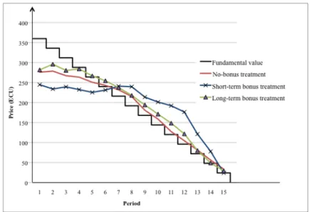
If the introduction of bonuses does not increase the likelihood of bubbles, it may influence the intensity of distorsions. We first consider the evolution of prices and trade volumes over time by treatment, before providing more formal measures of mispricing. Figure 2 displays the evolution of the median price over time by treatment. It shows that the median price is below the fundamental value in the first periods. Then, the median price exceeds it from between the fifth or the seventh period and the last periods. At first sight, the markets with short-term bonuses are associated with larger mispricing than the other treatments.
19
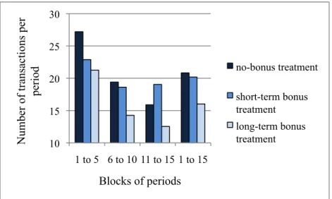
We also consider the evolution of the total volume of trades over time, as a high trade activity may be associated with mispricing. Figure 3 displays the evolution of the average trading volume by period for different blocks of periods and by treatment. We consider three blocks of periods: periods 1 to 5, periods 6 to 10, and periods 11 to 15. The last block on the right aggregates the data from all periods.
Figure 3. Evolution of the mean volume of trade per period for different blocks of periods, by treatment
Figure 3 shows that the average volume of trades is positive in each block of periods, with a declining time trend. The trading activity is always lower in the long-term bonus treatment than in the two other treatments, especially in the last block of periods. The difference between the long-term bonus treatment and the no-bonus treatment is all the more striking as the quantity of liquidities available is exactly the same in these two treatments throughout the session.
To complement this analysis, we use a range of standard summary measures of bubble severity from the literature on experimental asset markets. These measures include the normalized absolute price deviation (NAPD, hereafter), the normalized price deviation (NPD,
10 15 20 25 30 1 to 5 6 to 10 11 to 15 1 to 15 N um be r of t ra ns ac ti ons pe r pe ri od Blocks of periods no-bonus treatment short-term bonus treatment long-term bonus treatment
20
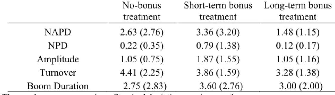
hereafter), the amplitude of price deviations, the turnover of assets, and the boom duration.16 The NAPD measures the per-share aggregate absolute deviation of the price from the asset fundamental value. A high normalized price deviation reflects high trading volumes and deviations of prices from fundamental values, indicating a market bubble (Haruvy and Noussair 2006). The NPD measure is similar to NAPD, except that instead of considering absolute price deviations, it relies on raw price deviations. It is close to the relative deviation defined by Stöckl, Huber and Kirchler (2010) except that our measure is normalized over the total sum of asset holdings. A positive NPD indicates that the market on average overvalues the asset, whereas a negative value indicates undervaluation. The amplitude measures the magnitude of overall price changes relative to the asset fundamental value throughout its life (King et al., 1993). Previous literature has shown that high amplitudes are associated with the presence of price bubbles. The turnover captures the intensity of the trading activity in the 15 periods (Smith et al., 1988). Finally, the boom duration represents the number of consecutive periods where the market median price is higher than the fundamental value by at least 20%. Table 1 displays the average values of these measures in each treatment.
Table 1 illustrates a consistent ranking of the three treatments. Mispricing seems to be more severe in the short-term bonus treatment than in the two other treatments. Indeed, for each measure except the turnover, the highest value is found in this treatment. In contrast, the long-term bonus treatment is associated with the lowest NAPD, NPD, amplitude and turnover. In this treatment, the mean boom duration lies in between the values for the two other treatments.
16 The formal definition of these measures can be found in Appendix B. Palan (2009) gives an extensive
presentation of the different measures of bubble severity, discusses the relative merits of each measure and presents the value of these measure obtained in previous studies.
21
Table 1. Summary characteristics of mispricing and asset turnover, by treatment No-bonus
treatment Short-term bonus treatment Long-term bonus treatment
NAPD 2.63 (2.76) 3.36 (3.20) 1.48 (1.15)
NPD 0.22 (0.35) 0.79 (1.38) 0.12 (0.17)
Amplitude 1.05 (0.75) 1.87 (1.55) 1.05 (1.16) Turnover 4.41 (2.25) 3.86 (1.59) 3.28 (1.38) Boom Duration 2.75 (2.83) 3.60 (2.76) 3.00 (2.00)
Note: The numbers are mean values. Standard deviations are in parentheses.
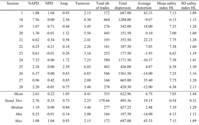
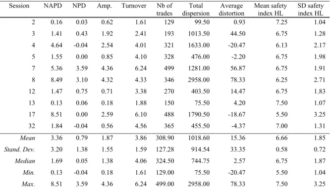
However, as typical in this type of games, there is a large heterogeneity in the dynamics of prices and market behavior across sessions within each treatment. The within-treatment heterogeneity is easily observable in Tables C1, C2 and C3 in Appendix C that display the same measures session by session. We next proceed to an econometric analysis of the data to analyze how the treatment manipulation and the composition of the pool of traders in each market influence mispricing and trading activity.
4.2. Econometric analysis
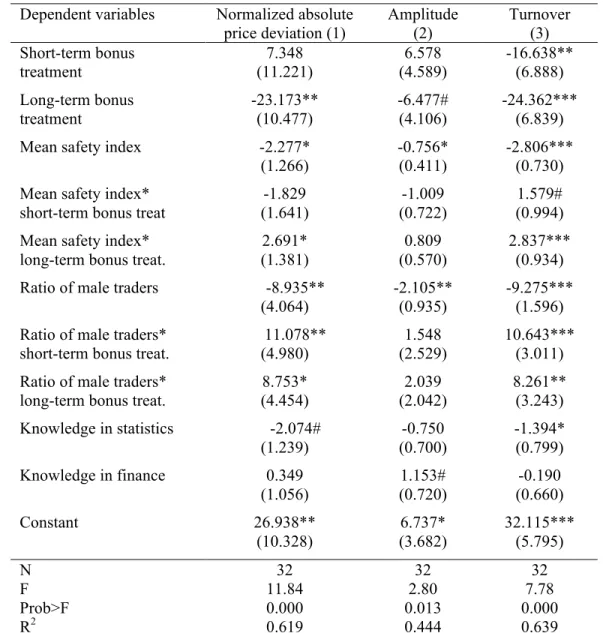
The determinants of measures of mispricing are estimated with Ordinary Least Squares models in which robust standard errors are clustered at the session level, as each session gives one independent observation. We pool the data of each treatment. Table 2 reports these estimates. To characterize the main dimensions of a bubble (price deviations, amplitude and market activity), the independent variables are the normalized absolute price deviation in model (1), the amplitude of bubbles in model (2) and the turnover of assets in model (3). To measure the impact of the treatment manipulation, the independent variables include dummy variables for each treatment in which bonuses have been introduced. The no-bonus treatment is taken as the reference category. To study whether the within-treatment heterogeneity in mispricing is driven by the traders’ characteristics in the market, we include
22
the mean traders’ degree of risk aversion as an independent variable. This aims at testing our conjecture 5. More precisely, we include the average safety index in each session. This index corresponds to the switching point in the Holt and Laury lottery choice task. The higher the average index is, the more risk-averse the traders on average are. We also include the ratio of male traders in each session. Indeed, gender differences have been often observed in financial decisions (Barsky et al., 1997; Powell and Ansic, 1997; Charness and Gneezy, 2007), with males being more overconfident than females (Barber and Odean, 2001) and less risk averse (see Croson and Gneezy, 2009, for a survey). Therefore, a higher proportion of males in a market may influence our measures. We allow both the mean level of risk attitudes and the gender ratio to vary across treatment by interacting these two variables with the dummy variables for each treatment. Finally, we control for the mean traders’ self-reported knowledge in statistics and finance in each session, as one could expect that a better average knowledge in these fields would reduce deviations from the equilibrium, other things equal.
Table 2 shows that, controlling for the characteristics of the pool of traders, the long-term bonus treatment generates lower price deviations (model (1)), a smaller amplitude of bubbles (significant only at the 12% level, see model (2)), and a lower turnover (model (3)) than the no-bonus treatment. Model (3) indicates that the asset turnover is also significantly lower in the short-term bonus treatment than in the no-bonus treatment. Similar regressions using the long-term bonus treatment as the reference category (not reported here but available upon request) indicate that price deviations and the amplitude of bubbles are significantly higher in the short-term bonus treatment than in the long-term bonus treatment (significant at the 1% level in both cases).
23
Table 2. Determinants of price deviations, amplitude and turnover Dependent variables Normalized absolute
price deviation (1) Amplitude (2) Turnover (3) Short-term bonus treatment 7.348 (11.221) 6.578 (4.589) -16.638** (6.888) Long-term bonus treatment -23.173** (10.477) -6.477# (4.106) -24.362*** (6.839)
Mean safety index -2.277*
(1.266)
-0.756* (0.411)
-2.806*** (0.730) Mean safety index*
short-term bonus treat
-1.829 (1.641) -1.009 (0.722) 1.579# (0.994) Mean safety index*
long-term bonus treat.
2.691* (1.381) 0.809 (0.570) 2.837*** (0.934) Ratio of male traders -8.935**
(4.064)
-2.105** (0.935)
-9.275*** (1.596) Ratio of male traders*
short-term bonus treat.
11.078** (4.980) 1.548 (2.529) 10.643*** (3.011) Ratio of male traders*
long-term bonus treat.
8.753* (4.454) 2.039 (2.042) 8.261** (3.243) Knowledge in statistics -2.074# (1.239) -0.750 (0.700) -1.394* (0.799) Knowledge in finance 0.349 (1.056) 1.153# (0.720) -0.190 (0.660) Constant 26.938** (10.328) 6.737* (3.682) 32.115*** (5.795) N F Prob>F 32 11.84 0.000 32 2.80 0.013 32 7.78 0.000 R2 0.619 0.444 0.639
Note: OLS models with robust standard errors clustered at the session level in parentheses. *** indicates significance at the 1% level, ** at the 5% level, * at the 10% level, # at the 12% level.
These findings support our conjecture 2 and are summarized in Result 2:
Result 2: The markets with long-term bonus contracts experience less price deviations,
smaller bubble amplitude than the markets with short-term bonus contracts and than the markets with no-bonus contracts.
24
Table 2 also indicates that the composition of the pool of traders influences both mispricing and turnover. Bubbles are less severe and trade activity is less intense in markets with more risk-averse traders. Indeed, there is a significant negative relationship between the mean safety index in the session, NAPD, amplitude and turnover. However, in the long-term bonus treatment, the net impact of risk attitudes on both NAPD and turnover is negligible as the variable interacting the mean risk attitudes and the treatment dummy receives almost the same but positive coefficient as the mean safety index variable (see models (1) and (3)). This suggests that when long-term bonuses are at stake, the positive relationship between the behavior of more risk-seeking traders and mispricing vanishes out almost completely.
Last, we observe that in the no-bonus treatment a higher proportion of male traders is associated with lower NAPD, amplitude of bubbles, and turnover. However, the gender composition of the pool of traders has a neutral net impact in the long-term bonus treatment. And in the short-term bonus contracts, a higher ratio of male traders even generates a net positive impact on NAPD and asset turnover. A possible interpretation is related to the fact that bonus contracts are competitive incentives and that competition is more intense and salient when bonuses are at stake in each period. Previous literature has shown that males are much more competitive than females (Gneezy et al., 2003; Niederle and Vesterlund, 2007; Villeval, 2012). Therefore, male traders may behave more actively in the market when bonuses are at stake –especially when assigned each period- than in the absence of bonuses. This analysis supports partly our conjectures 1 and 5 and leads to the following results:
Result 3: Mispricing is less severe and trade activity is less intense in markets with more
risk-averse traders and a higher share of male traders, except when competitive incentives are at stake and especially when bonuses are assigned each period.
25
Result 4: Markets with short-term bonus contracts tend to exhibit higher price deviations than
the markets with no bonuses and the markets with long-term bonus contracts but only when they involve a higher share of male traders.
4.3. Risk attitudes and individual behavior
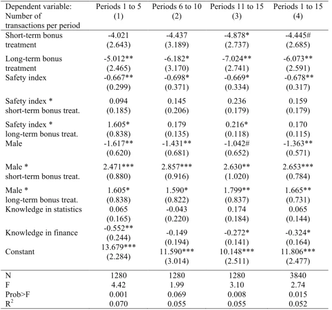
In this sub-section, we study whether risk attitudes influence individual trading activity and the subsequent earning of bonuses. Table 3 displays the results of regressions in which the dependent variable is the trader’s number of transactions per period. To study whether risk attitude has a different impact on trading activity depending on the phase of the market (bubble formation, boom and crash), model (1) considers periods 1 to 5; model (2) periods 6 to 10, model (3) periods 11 to 15, and model (4) is for the whole market. These models are estimated by Generalized Least Squares models with robust standard errors clustered at the session level. The independent variables include dummy variables for each treatment with bonuses, with the no-bonus treatment taken as the reference category. They also include the trader’s individual safety index and gender. These variables are interacted with dummy variables for each treatment with bonuses as we suspect that risk attitudes and gender may have a different impact when bonuses are offered. Finally, two variables capture the self-reported knowledge in statistics and finance.
Table 3 shows that traders have a significantly lower activity in the long-term bonus treatment than in the other treatments and the value of the associated coefficient increases over time. Supporting conjecture 3 and our previous analysis, it also shows that more risk averse traders are less active in the market, regardless of the block of periods considered. But contrary to our conjecture 4, the introduction of bonuses does not affect the impact of risk aversion on trading activity in the short-term treatment. The (marginal) impact of risk aversion is even sometimes reverted in the long-term bonus treatment, where less risk-averse individuals are less willing to
26
trade. Confirming the analysis at the market level, males trade significantly less than females in almost all blocks of periods. However, the introduction of long-term bonuses annihilates this effect while the net joint effect of short-term bonuses and male gender is positive. An interpretation is that in the presence of short-term incentives, males’ competitiveness is increased. Finally, a better knowledge in finance tends to limit trading activity in most blocks of periods.
Table 3. Individual determinants of activity in the market in various blocks of periods Dependent variable:
Number of
transactions per period
Periods 1 to 5 (1) Periods 6 to 10 (2) Periods 11 to 15 (3) Periods 1 to 15 (4) Short-term bonus treatment Long-term bonus treatment Safety index Safety index * short-term bonus treat. Safety index * long-term bonus treat. Male
Male *
short-term bonus treat. Male *
long-term bonus treat. Knowledge in statistics Knowledge in finance Constant -4.021 (2.643) -5.012** (2.465) -0.667** (0.299) 0.094 (0.185) 1.605* (0.838) -1.617** (0.620) 2.471*** (0.880) 1.605* (0.838) 0.065 (0.165) -0.552** (0.244) 13.679*** (2.284) -4.437 (3.189) -6.182* (3.170) -0.698* (0.371) 0.145 (0.206) 0.179 (0.135) -1.431** (0.681) 2.857*** (0.916) 1.590* (0.822) -0.043 (0.220) -0.149 (0.194) 11.590*** (3.014) -4.878* (2.737) -7.024** (2.741) -0.669* (0.334) 0.236 (0.179) 0.216* (0.118) -1.042# (0.652) 2.630** (1.020) 1.799** (0.837) 0.174 (0.184) -0.272* (0.141) 10.148*** (2.511) -4.445# (2.685) -6.073** (2.591) -0.678** (0.317) 0.159 (0.179) 0.170 (0.115) -1.363** (0.571) 2.653*** (0.784) 1.665** (0.731) 0.065 (0.144) -0.324* (0.164) 11.806*** (2.477) N F Prob>F R2 1280 4.42 0.001 0.070 1280 1.99 0.069 0.055 1280 3.10 0.008 0.055 3840 2.74 0.015 0.052
Note: GLS models with robust standard errors clustered at the session level in parentheses. *** indicate significance at the 1%
27 These findings are summarized in the following results:
Result 5: At the individual level, a higher degree of risk aversion and a better knowledge in
finance reduce trading activity.
Result 6: At the individual level, controlling for risk preferences, introducing competitive
incentives –especially short-term bonuses- increases male traders’ activity.
Finally, we study whether the degree of risk aversion and gender predict the bonuses earned by the traders in the market in the short-term and the long-term bonus treatments. Table 4 reports the estimates of four ordered probit models with robust standard errors clustered at the market level in which the dependent variable is the amount of the bonus received in each period in the short-term bonus treatment. The ordered probit model is justified since individuals can earn either no bonus or one of three possible bonuses. Model (1) corresponds to periods 1 to 5, model (2) to periods 6 to 10, model (3) to periods 11 to 15, and model (4) is for the whole market (periods 1 to 15). Model (5) in Table 4 analyzes the individual determinants of the receipt of bonuses in the long-term bonus treatment. It is also estimated by means of an ordered probit model with clustering at the session level. The independent variables in all models are the trader’s individual safety index, gender, and self-reported knowledge in statistics and in finance.
Models (1) and (2) identify a significant relationship between the trader’s risk attitude and gender and the bonuses earned in the first ten periods of the short-term bonus treatment (confirmed by model (4) for the whole market). In this block of periods, both a higher degree of individual risk aversion and being a male trader are associated with a higher probability to earn higher bonuses.
28
Table 4. Determinants of the receipt of bonuses in a period Dependent variable: Short-term bonus treatment Amount of bonus earned Periods 1-5 (1) Periods 6-10 (2) Periods 11-15 (3) Periods 1-15 (4) Long-term bonus treatment (5) Safety Index Male Knowledge in statistics Knowledge in finance 0.128*** (0.037) 0.357** (0.159) 0.018 (0.124) 0.067 (0.076) 0.074*** (0.029) 0.370** (0.182) 0.063 (0.067) -0.040 (0.066) 0.005 (0.022) 0.039 (0.170) -0.060 (0.055) -0.023 (0.036) 0.067*** (0.013) 0.248** (0.102) 0.006 (0.062) 0.001 (0.048) 0.064 (0.070) 0.001 (0.334) 0.318 (0.219) -0.117 (0.173) N Wald chi2 23.85 400 15.27 400 2.99 400 30.60 1200 3.36 80 Prob>chi2 0.000 0.004 0.560 0.000 0.499 Pseudo R2 0.035 0.020 <0.001 0.011 0.029 log pseudo-likelihood -414.347 -420.804 -428.346 -1274.705 -83.388
Note: Ordered probit models, with robust standard errors clustered at the session level in parentheses. ***
indicate significance at the 1% level and ** at the 5% level.
In contrast, risk attitudes and gender do not affect the amount of bonuses earned in the last five periods. This may result from the fact that this phase of the market corresponds to bubble bursts and is quite chaotic both for prices and transactions. Players with a higher degree of risk aversion and a higher competitiveness are better able to profit from the market opportunities. Including the volume of traded assets by the individual in the regressions does not affect the probability of receiving bonuses (regressions available upon request). Finally, we do not observe any significant impact of risk attitudes and gender on the receipt of bonuses in the long-term bonus treatment. This leads to our final result:
Result 7: Risk-averse traders and male traders are more likely to earn bigger bonuses in the
29 4. CONCLUSION
This paper has explored the effects of various incentive contracts for traders on the evolution of prices and on trading activity in experimental asset markets. Consistent with the previous literature, our treatment with no bonus exhibits active trading and persistent deviations of prices from the assets’ fundamental values. If competitive incentives do not increase the likelihood of bubbles, the markets with long-term bonuses experience the lowest price deviations, amplitude and turnover of assets. Mispricing and turnover of assets are even smaller than in the markets with no bonuses. This is in contrast with the conclusions of Isaac and James (2000, 2003), probably due to the use of a different rule for selecting the winners of the tournament. The markets with short-term bonuses experience higher price deviations, amplitude and boom duration than the two other types of markets; however, mispricing is significantly more severe only when the market involves a higher share of male traders.
Although we are cautious not extrapolating our results due to the heterogeneity of behavior across markets, they provide some evidence that the rules for determining traders’ compensation matter in the evolution of prices and trade volumes. In particular, the long-term bonuses contribute to reduce market inefficiency by reducing the volume of trades and mispricing probably because these bonuses reinforce the assets’ final fundamental value as a focal point from the very beginning of the market, while the short-term bonuses make bonuses and current prices more salient than the fundamental value of the assets. This reveals the importance of the reference point introduced by compensation policies on behavior.
Previous studies report that experience (Dufwenberg et al., 2005), detailed exposure of the fundamental value evolution (Lei and Vesely, 2009), context presentation (Kirchler et al., 2012) or public knowledge on appropriate training (Cheung et al., 2012) reduce the occurrence and the severity of bubble in experimental asset markets. Nevertheless, the creation
30
of bubbles in an environment where traders are informed from the beginning of the evolution of the fundamental value of the assets remains an interesting research topic for economists. Testing whether the composition of the pool of traders affects the dynamics of trades and prices on the markets, we have found that mispricing is more severe and trading activity is more intense in markets where the pool of traders is on average less risk-averse. The introduction of short-term bonuses increases the impact of gender on trading behavior and on mispricing, possibly due to the reinforcing effect of these incentives on males’ competitiveness. A potential implication of these findings is that educating individuals in risk management could contribute to reduce the severity of distorsions in asset markets.
Several extensions could be thought of. With our design, we cannot exclude that the amount of short-term bonuses infused in the market contributes to mispricing. Therefore, we could explore whether the extent of mispricing would differ if the bonuses earned throughout the game would be kept in a private account and could not be used to trade. Another extension could consist of measuring how a richer set of information (including for example the distribution of performances in the period) would affect market behavior.
31
REFERENCES
Ang, J.S., Schwartz, T. (1985). Risk aversion and information structure: An experimental study of price variability in the securities markets. Journal of Finance 40, 825-844.
Barber, B.M., Odean, T. (2001). Boys Will Be Boys: Gender, Overconfidence, and Common Stock Investment. The Quarterly Journal of Economics 116 (1), 261-292.
Barsky, R., Juster, F., Kimball, M., Shapiro, M. (1997) Preference Parameters and Behavioral Heterogeneity: An Experimental approach in the Health and Retirement Study. The
Quarterly Journal of Economics 112 (2), 537-579.
Becker, B.E., Huselid, M.A. (1992). The Incentive Effects of Tournament Compensation Systems. Administrative Science Quarterly 37 (2), 336-350.
Bronars, S. (1986). Strategic Behavior in Tournaments, Texas A&M University, Austin, mimeo.
Brown, K.C., Harlow W.V., Starks, L.T. (1996). Of Tournaments and Temptations: An Analysis of Managerial Incentives in the Mutual Fund Industry. Journal of Finance 51 (1), 85-110.
Busse, J.A. (2001). Another Look on Mutual Funds Tournaments, Journal of Financial and
Quantitative Analysis 36(1), 2001, 53–73.
Caginalp, G., Porter, D.P., Smith, V.L. (1998). Initial Cash/Asset Ratio and Asset Prices: An Experimental Study, Proceedings of the National Academy of Sciences 95, 756–761. Caginalp, G., Porter, D.P., Smith, V.L. (2001). Financial bubbles: excess cash, momentum,
and incomplete information, Journal of Psychology and Financial Markets 2(2), 80–99. Charness, Gary B., Gneezy, U. (2007). Strong Evidence for Gender Differences in Investment.
University of California at Santa Barbara, Economics Working Paper Series, Department of Economics, UC Santa Barbara. http://www.escholarship.org/uc/item/428481s8.
Cheung, S., Palan, S. (2012). Two heads are less bubbly than one: team decision-making in an experimental asset market, Experimental Economics 15(3), 373-397.
Cheung, S., Coleman, A. (2011). League-Table Incentives and Price Bubbles in Experimental Asset Markets, IZA Discussion Paper 5704, Bonn.
Cheung, S. L., Hedegaard, M., & Palan, S. (2012). To See Is To Believe: Common Expectations in Experimental Asset Markets, IZA Discussion Paper 6922, Bonn.
Chevalier, J., Ellison, G. (1997). Risk taking by mutual funds as a response to incentives,
Journal of Political Economy 105, 1167-1200.
Croson, R., Gneezy, U. (2009). Gender Differences in Preferences. Journal of Economic
Literature 47 (2), 448–474.
Dufwenberg, M., Lindqvist, T., & Moore, E. (2005). Bubbles and Experience: An Experiment,
American Economic Review, 95, 1731-1737.
Fama, E.F. (1970). Efficient Capital Markets: A Review of Theory and Empirical Work, The
32
Fellner, G., Maciejovsky, B. (2007). Risk attitude and market behavior: Evidence from experimental asset markets, Journal of Economic Psychology, 28, 338-350.
Fischbacher, U. (2007). Z-Tree: Zurich Toolbox for Ready-made Economic Experiments,
Experimental Economics, 10, 171-178.
Friedman D. (1993). The Double Oral Auction Market Institution: A Survey, In The
Continuous Double Auction Market: Institutions, Theories, and Evidence, ed. D.
Friedman and J. Rust, 3-26. Reading Mass.: Addison-Wesley.
G20 Leaders (2009). G20 Leaders Statement: The Pittsburgh Summit, September 24-25, 2009, Pittsburgh Retrieved from URL
Gaba, A., Kalra, A. (1999). Risk Behavior in Response to Quotas and Contests, Marketing
Science 18 (3), 417-434.
Gneezy, U., Niederle,M., Rustichini, A. (2003). Performance in Competitive Environments: Gender Differences. The Quarterly Journal of Economics, 118, 1049–1074.
Greiner, B. (2004). An online recruitment system for economic experiments. In Forschung und wissenschaftliches Rechnen GWDG Bericht 63, Ed. K. Kremer, and V. Macho. Göttingen: Gesellschaft für Wissenschaftliche Datenverarbeitung.
Güth, W., Krahnen, J.P., Rieck, C. (1997). Financial markets with asymmetric information: A pilot study focusing on insider advantages, Journal of Economic Psychology 18, 235-257. Haruvy, E., Noussair, C.N. (2006). The Effect of Short-Selling on Bubbles and Crashes in
Experimental Spot Asset Markets, Journal of Finance 61 (3), 1119-1157.
Holt, C.A., Laury, S.K. (2002). Risk Aversion and Incentive Effects, American Economic
Review 92(5), 1644-1655.
Hvide, H.K. (2002). Tournament Rewards and Risk Taking, Journal of Labor Economics 20, 877-898.
Isaac, M.R., James, D. (2003). Boundaries of the Tournament Pricing Effect in Asset Markets: Evidence from Experimental Markets, Southern Economic Journal 69 (4), 2003, 936-951. James, D., Isaac, M.R. (2000). Asset Market Efficiency: the Effects of Tournament Incentives
for Individuals, American Economic Review 90, 995-1004.
Kempf, A., Ruenzi, S. (2008). Tournaments in Mutual-Fund Families, Review of Financial
Studies 21 (2), 1013-1036.
King, R.R., Smith, V.L., Williams, A.W., Van Boening, M. (1993). The robustness of bubbles
and crashes in experimental stock markets. In Day, R., Chen, P. (Eds.), Nonlinear Dynamics and Evolutionary Economics. Oxford: Oxford University Press, 183 -200.
Kirchler, M., Huber, J., Stöckl, T. (2012). Thar she bursts – Reducing confusion reduces bubbles, American Economic Review, 102(2), 865-883.
Lee, J. (2004). Prize and Risk-Taking Strategy in Tournaments: Evidence from Professional Poker Players, IZA Working Paper 1345, Bonn.
33
Lei, V., Noussair, C.N., Plott, C.R. (2001). Nonspeculative Bubbles in Experimental Asset Markets: Lack of Common Knowledge of Rationality vs. Actual Irrationality,
Econometrica 69 (4), 831-859.
Lei, V., Vesely, F. (2009). Market efficiency: evidence from a no-bubble asset market experiment, Pacific Economic Review, 14, 246-258.
McLaughlin, K.J. (1988). Aspects of Tournament Models: A Survey, in Research in Labor
Economics, JAI Press, 225–256.
Milgrom, P., Stokey, N. (1982). Information, trade and common knowledge, Journal of
Economic Theory 26 (1), 17-27.
Niederle, Muriel and Vesterlund, Lise, (2007). Do Women Shy Away from Competition? Do Men Compete Too Much? The Quarterly Journal of Economics 122 (3), 1067-1101. Nieken, P. Sliwka, D. (2010). Risk-taking Tournaments – Theory and Experimental Evidence.
Journal of Economic Psychology 31 (3), 254-268.
Noussair, C., Robin, S., Ruffieux, B. (2001). Price Bubbles in Laboratory Asset Markets with Constant Intrinsic Values, Experimental Economics 4, 87-105.
Oechssler, J., Schmidt, C., Schnedler, W. (2011). On the Ingredients for Bubble Formation: Informed Traders and Communication, Journal of Economic Dynamics and Control, 35(11), 1831–1851.
Palan, S. (2009). Bubbles and Crashes in Experimental Asset Markets, Lecture Notes in Economics and Mathematical Systems, vol. 626, Springer, Heidelberg et al.
Palomino, F. (2005). Relative Performance Objectives in Financial Markets, Journal of
Financial Intermediation 14, 351-375.
Powell, M., Ansic, D. (1997). Gender Differences in Risk Behavior in Financial Decision-Making: An Experimental Analysis. Journal of Economic Psychology 18, 605-628.
Qui, J. (2003). Termination Risk, Multiple Managers and Mutual Fund Tournaments,
European Finance Review 7, 161-190.
Smith, V.L., Suchanek, G.L., Williams, A.W. (1988). Bubbles, Crashes, and Endogenous Expectations in Experimental Spot Asset Markets, Econometrica 56(5), 1119-1151. Smith, V.L., van Boening, M. Wellford, C.P. (2000). Dividend Timing and Behavior in
Laboratory Asset Markets, Economic Theory 16(3), 567-83.
Stöckl, T., Huber, J., Kirchler, M. (2010). Bubble measures in experimental asset markets,
Experimental Economics 13, 284-298.
Sutter, M., Huber, J., Kirchler, M. (2012). Bubbles and information : an experiment,
Management Science 58, 384-393.
Taylor, J. (2003). Risk-taking behavior in mutual fund tournaments, Journal of Economic
Behavior & Organization 50, 373-383.
Tirole, J. (1982). On the Possibility of Speculation under Rational Expectations, Econometrica 50 (5), 1163-1182.
34
Van Boening, M. V., Williams, A. W., & LaMaster, S. (1993). Price bubbles and crashes in experimental call markets. Economics Letters, 41 (2), 179-185.