HAL Id: ird-01822368
https://hal.ird.fr/ird-01822368
Submitted on 8 Mar 2019
HAL is a multi-disciplinary open access
archive for the deposit and dissemination of sci-entific research documents, whether they are pub-lished or not. The documents may come from teaching and research institutions in France or abroad, or from public or private research centers.
L’archive ouverte pluridisciplinaire HAL, est destinée au dépôt et à la diffusion de documents scientifiques de niveau recherche, publiés ou non, émanant des établissements d’enseignement et de recherche français ou étrangers, des laboratoires publics ou privés.
Analysis of haplotype networks: the randomized
minimum spanning tree method
Emmanuel Paradis
To cite this version:
Emmanuel Paradis. Analysis of haplotype networks: the randomized minimum spanning tree method. Methods in Ecology and Evolution, Wiley, 2018, 9 (5), pp.1308 - 1317. �10.1111/2041-210X.12969�. �ird-01822368�
January 5, 2018
Analysis of haplotype networks: the randomized minimum
spanning tree method
Emmanuel Paradis
ISEM, IRD, Univ. Montpellier, CNRS, EPHE, Montpellier, France
Summary
1. Haplotype network construction is a widely used approach for analysing and visualising the relationships among DNA sequences within a population or
3
species. This approach has some problems such as how to quantify alternative links among sequences, or how to plot efficiently networks to compare them easily. 2. In this paper, a new method is presented: the randomized minimum spanning tree
6
method, based on randomizing the input order of the data in order to produce alternative branchings in the haplotype network. It is shown that this new method can produce, at least in some situations, networks with less alternative links than
9
the minimum spanning network method.
3. A new graphical display of haplotype networks is introduced here. This is based on calculating the coordinates of the haplotypes from a multidimensional scaling
12
of the haplotype distance matrix. The display can be done in two or three
dimensions. The eigenvalues extracted from the multidimensional scaling analysis give an indication of the relevant number of dimensions.
15
4. These tools are illustrated with the analyses of published data on the leopard and on the jaguar. These analyses show interesting and contrasting patterns between these two species of big cats.
18
5. All tools are implemented in R and available in the packagepegas.
Keywords: Hamming distance, haplotype network, microevolution, minimum spanning tree, Panthera
Introduction
The analysis of DNA sequences from individuals sampled in one or several populations makes possible to address different questions on microevolutionary processes such as
24
population structure, gene flow, past demographic bottlenecks and expansions, or
geographical events of colonizations and extinctions (Bossart & Prowell, 1998; Emerson et al., 2001; Buerkle & Lexer, 2008). An important aspect of these analyses is the
27
inference of ancestry–descendance relationships among haplotypes. Typically, if the sequences are assumed to be contemporaneous, two alternative approaches can be adopted: inferring either a phylogenetic tree, or a network. The phylogenetic approach
30
assumes that the ancestral sequences are unobserved and associated with the internal nodes of the tree while the observed sequences are associated with its terminal nodes. On the other hand, if some observed sequences may be ancestral to others, a network
33
approach is more appropriate, in which case these sequences will be associated with the internal nodes of the network. It is clear that choosing an approach or the other will depend on the time frame and the mutation rate of the sequences. If the sequences are
36
sampled sequentially through time (e.g., pathogens sampled through an epidemic, or ancient DNA), several approaches have been developed to take this temporal dimension into account (e.g., Jombart et al., 2011).
39
Network methods can be classified according to different criteria (Table 1). For instance, it is possible to define two categories depending on their main objective: the ‘explicit’ networks depict reticulated processes of evolution such as hybridization,
42
horizontal gene transfer, or admixture, whereas the ‘implicit’ networks represent some form of uncertainty over a tree (i.e., without reticulation) representation (Huson & Bryant, 2006; Kloepper & Huson, 2008). Another way to classify network methods
45
considers the reconstruction method: these include parsimony, distances, maximum likelihood, Bayesian inference, split decomposition, or consensus methods (Holland
et al., 2004). Another important criterion is whether unobserved haplotypes can be
48
included in the network: distance-based methods cannot generally do this because they do not consider explicitly the evolving characters (Table 1). It is crucial to assess the reliability of a phylogeny or network of haplotypes since its construction may be affected
51
by sampling biases (i.e., missing haplotypes). A badly estimated network is likely to lead to wrong inference of population or history.
The present paper focuses on the distance-based, implicit network approach. Two
54
methods are commonly used to build a haplotype network: the minimum spanning tree (MST) method (Kruskal, 1956) and the method from Templeton et al. (1992, TCS). The MST method has been applied in many fields (Neˇsetˇril et al., 2001). Its principle is to
57
first build a matrix of pairwise distances among sequences (or haplotypes), and then find the shortest set of paths that link all observations where the length of each link is taken from the pairwise distance. The TCS method, often referred to as statistical parsimony,
60
is based on a model of evolution of the genetic characters measured on each
individual—originally restriction fragment lengths but the method can be applied to DNA sequences. The main difference between both methods is that an MST is a network
63
with no reticulation, thus for n sequences, the resulting MST will have n − 1 links. On the other hand, a TCS network may have reticulations defining alternative branchings, and include unobserved haplotypes in the network. Thus, this method may be used to
66
infer micro-evolutionary events such as putative recombinations (Posada & Crandall, 2001). Bandelt et al. (1999) developed another method called the median-joining network (MJN) where alternative branchings are found by examining potential ancestral
69
sequences for each triplet of sequences. MJN belongs to a class of methods which includes several variants such as reduced median network or quasi-median network (Bandelt et al., 1995, 1999). Thus, the MST usually cannot represent possible
72
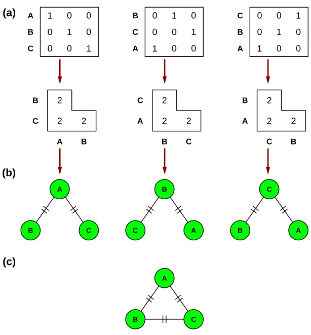
for a given data set, the MST may not be unique. Figure 1 shows a simple illustration of this problem: the three represented data sets are identical but the inferred MSTs are
75
different because the observations are ordered differently. This is a consequence of the presence of ties in the distance matrix (see the algorithm descriptions below). With real data, this problem and its consequences may be very hard to detect with a large number
78
of observations. Bandelt et al. (1999) pointed out that instead of constructing a single tree, it is possible to construct a minimum spanning network (MSN) by modifying slightly Kruskal’s (1956) algorithm as explained below.
81
In this paper, I propose a new algorithm to construct a network which can be seen as intermediate between the MST and MSN methods. I also present tools to compare networks programmed in R (R Core Team, 2017).
84
Methods
MINIMUM SPANNING TREE AND NETWORK
The MST algorithm can be sketched as follows (Kruskal, 1956):
1. Compute the matrix of pairwise distances among the n observations and sort them
87
in increasing order.
2. Assign each observation to its own group; there are thus n initial groups. 3. Set i ← 1.
90
4. Take the ith distance from step 1: if the two corresponding observations are not in the same group, then create a link between them and pool the two groups.
5. Set i ← i + 1.
93
The number of groups is decreased by one at each iteration of step 4. The issue with this algorithm is how ties in the distance matrix are treated in step 1, and this is, obvioulsy,
96
dependent on the implementation. The MSN tries to solve this problem (Bandelt et al., 1999); its algorithm is:
1. Compute the matrix of pairwise distances among the n observations, extract the
99
unique values, and sort them in increasing order (denoted as δ1, δ2, . . .).
2. Set i ← 1.
3. Create the links for all pairs of observations with distance equal to δi.
102
4. If all observations are linked in a single group, then stop. 5. Set i ← i + 1, and go to step 3.
THE RANDOMIZED MINIMUM SPANNING TREE
The input data are a set of aligned sequences from which a distance matrix is computed.
105
The sequences could be DNA or other kinds as long as there is a method to compute pairwise distances. In most applications, a simple Hamming distance (or Manhattan in the case of binary characters) will be relevant. In order to remove the influence of the
108
order of the input data, the procedure is based on a randomization of this order. This is repeated many times and for each replication an MST is constructed. The MSTs are then post-processed in order to return a single network including all the links observed among
111
the replications. Because of the nature of the proposed algorithm, it is called here the randomized minimum spanning tree(RMST) method.
The RMST usually has less links than the MSN. Figure 2 shows a simple example
114
with four binary sequences. The first step of the network construction is to consider links of length one A–C and A–B; the second step considers the links of length two A–D and
B–C. During the MST construction, the link B–C is never included because B and C
117
were already grouped together during the first step, so the RMST does not include this link. On the other hand, the MSN includes this link thus resulting in two alternative paths, B–A–C and B–C, both of the same length. The RMST avoids this ambiguity. Note
120
the difference between the present example and the one in Figure 1: in the latter, the additional link output by the MSN creates a path shorter than the one created by the MST.
123
GRAPHICAL TOOLS
Plotting networks is a notoriously difficult problem (e.g., Kloepper & Huson, 2008). Several computer programs perform graphical display of various types of evolutionary networks, such as igraph (Csardi & Nepusz, 2006), network (Butts, 2008), phangorn
126
(Schliep, 2011), pegas (Paradis, 2010), or SplitsTree (Huson, 1998), among many others. In practice, it would be very useful to graphically compare networks constructed under different methods or assumptions. However, this is usually not possible (or very difficult)
129
because there is no standard procedure for plotting haplotype networks. To propose a solution to this problem, an implementation based on multidimensional scaling (MDS; Torgerson, 1952) is developed here. The procedure is to first perform an MDS on the
132
distance matrix in order to extract two or three sets of coordinates. These coordinates are then used to plot the observed sequences or haplotypes in 2-D or in 3-D, and the links inferred from the network are then drawn. Thus, this procedure contrasts with most
135
existing ones which compute the layout of haplotypes trying to minimize line crossings (e.g., Kloepper & Huson, 2008). The proposed procedure has several advantages. First, an MDS on the original distance matrix will arrange the sequences depending on their
138
similarity. Second, the eigenvalues extracted from the MDS make possible to assess whether it is relevant to use two or three dimensions in this projection. Third, the
coordinates of the observations will be the same for all networks since they depend only
141
on the distance matrix, making graphical comparisons easier. Fourth, the procedure is computationally straightforward since an MDS is usually fast to perform even with several hundreds observations.
144
The tools presented in this article have been implemented in the R packagepegas
(Paradis, 2010). This package has already implemented a standard 2-D plot using an “energy-minimisation” algorithm to optimise the layout. Plots in three dimensions have
147
been implemented using therglpackage (Adler et al., 2016).
SIMULATION STUDY
To assess how the RMST is able to find alternative links in a network of haplotypes, some simulations were run under different situations of mutation rate (µ), sequence
150
length (l), and number of sequences (n). A set of n sequences was simulated under the JC69 model of sequence evolution (Jukes & Cantor, 1969) along a random network with no reticulation and link lengths taken from a standard uniform distribution. The network
153
was simulated by generating a random binary tree where the internal nodes were considered contemporaneous to the leaves. The sequences were then analysed with the RMST using different numbers of randomizations (5, 10, 20, 50, 100): the number of
156
additional links found by the RMST as well as the number of unique distances were recorded. The other parameters were: n = 50, 100, 500, or 1000, l = 500 or 1000, and µ= 0.01 or 0.1. These parameter values were chosen to result in substantial numbers of
159
ties in the distance matrices. The simulations were replicated 100 times for each
DATA
Two data sets were considered to apply the methods introduced in this paper: a set of
162
mtDNA sequences from 33 leopards (Panthera pardus) published by Uphyrkina et al. (2001), and a set of mtDNA sequences from 37 jaguars (P. onca) published by Eizirik et al.(2001). Both data sets were downloaded from GenBank (accession numbers:
165
AY035227–AY035292 and AF244814–AF244887, for each species, respectively). The sequences were aligned separately for the different genes (using information from GenBank and from the original publications) with MUSCLE (Edgar, 2004), and then
168
combined into two global alignments with 726 and 707 sites, respectively. All sequences were unique for the leopard data, but 22 unique sequences were identified for the jaguar data. For each alignment, a matrix of Hamming distances was calculated withape
171
(Paradis et al., 2004). These matrices were used as input for the construction of the networks. The individual labels from the original studies were kept for the present analyses. The R scripts used for these analyses is provided in the Supplementary
174
Information.
Results
SIMULATION STUDY
To simplify the presentation of the results, the number of additional links was calculated
177
as successive differences with increasing number of randomizations (i.e., the numbers of links found with five randomizations compared to zero, with ten randomizations
compared to five, and so on). The results were clearly related to the number of unique
180
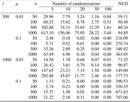
distances among the simulated distances. Considering that the total number of distances is given by n(n − 1)/2, the percentage of unique distances was always less than 1% (Table 2). Increasing l and/or µ resulted in more variation among the sequences and,
consequently, less additional links for the same n. On the other hand, increasing n for the same values of l and µ resulted in more closely related sequences, and thus more
additional links found by the RMST. In three cases, some additional links were still
186
found with 100 randomizations. In the scenario simulating the most diversity (l = 1000, µ= 0.1), five randomizations were enough to find the additional links of the RMST for all values of n.
189
APPLICATION
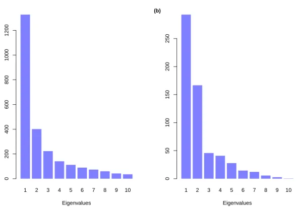
The MDS analysis of the distance matrices resulted in slightly different patterns of eigenvalues. For the leopard data, the first eigenvalue was much larger than the others though the second and third ones were substantially larger than the remaining ones
192
(Fig. 3a). For the jaguar data, the first and the second eigenvalues were much larger than all the other ones (Fig. 3b). Thus, we may anticipate that three dimensions may represent the distribution of sequences for the leopard data whereas two dimensions may be
195
enough for the jaguar data.
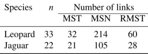
The MSN and RMST analyses revealed large numbers of additional links compared to the MST ones (Table 3). In the case of the leopards, the number of links was
198
multiplied by 6.7 from the MST to the MSN, and by 1.9 to the RMST. This increase in number of links was slightly smaller in the case of the jaguar: 5 to the MSN and 1.3 to the RMST. The RMST analyses were repeated with different numbers of
201
randomizations. For the leopard data, 59 links were found with 10 randomizations while 60 links were found with 50 randomizations or more. For the jaguar data, 28 links were found with 10 randomizations or more.
204
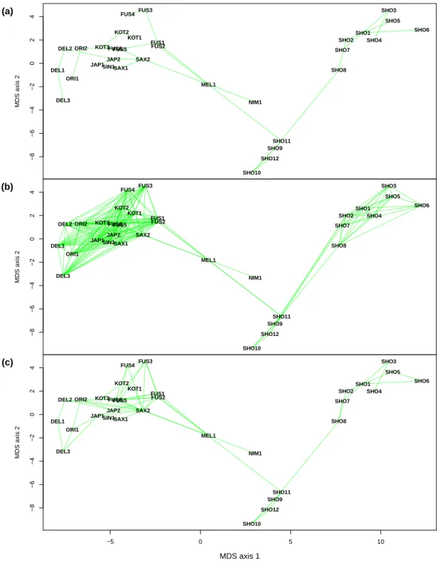
The MDS-based plots of the leopard sequences showed a clear continental separation with the African individuals (SHO*) on the right-hand side of the plot, and the Asian ones on the left-hand side (Fig. 4). Interestingly, two individuals laid outside of these
two groups: the one from the Arabian Peninsula (NIM1) and the one from Java, Indonesia (MEL1). Remarkably, the RMST did not add any further link from NIM1 to the others, whereas two additional links were observed between MEL1 and the Asian
210
ones. The MSN kept NIM1 with a single link to SAX2, but added one further link between MEL1 and the others. The 3-D displays revealed that the African individuals, which are apparently aligned in the 2-D plots, are actually arranged along an arc in the
213
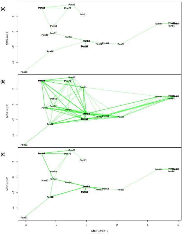
third dimension of the MDS (videos provided in the Supplementary Information). For the jaguar data, the arrangement of the individuals on the first axis followed a North–South axis with individuals from the South on the right-hand side of the plot
216
(Fig. 5). Two individuals remained single-linked with the MSN and RMST analyses: Pon23 from Nicaragua which was linked with two individuals from Nicaragua and from Costa Rica, both with the same haplotype, and Pon63 from Venezuela which was linked
219
with Pon73, an individual of unknown origin but presumably from Brazil (Eizirik et al., 2001). Except for Pon63, very little dispersion was observed in the third dimension as expected from the eigenvalues of the MDS (videos provided in the Supplementary
222
Information).
Discussion
The analysis of the relationships among DNA sequences and haplotypes within and
225
among populations is crucial for testing hypotheses on microevolutionary processes. However, such analyses often suffer from shortcomings. Typically, two issues are often observed. First, practitioners usually construct a single haplotype network which is then
228
interpreted depending on the context of the study. This can be a problem when the assumptions of the method are not met, which can usually be assessed by comparing different constructions, for instance, by using different distances. The second problem is
231
to read “minimum spanning network” when an MST is obviously shown since no loop is present. This is problematic since the MST may not be unique as already mentioned by
234
Bandelt et al. (1999).
The RMST method is an alternative to the MSN with the advantage of creating less links among haplotypes while fully taking into account the ambiguities induced by data
237
ordering. In the applications with real data presented in this paper, 100 randomizations were done and the results were identical than with smaller numbers. The computing times of the method is thus proportional to the product of n (since n − 1 links are built at
240
each replication of the MST algorithm) with the number of randomizations. The implementation inpegasresamples the distance matrix by reordering its rows and columns simultaneously, instead of reordering the original data matrix, and thus avoids
243
to recalculate the distance matrix at each iteration of the MST (which requires a computing time proportional to n2).
The simulation study showed that the number of randomizations required to reach
246
convergence of the RMST procedure is affected by the number of sequences, the sequence length, and the mutation rate. Because it is not easy to define a priori how many randomizations are required for a given data set, it is recommended to repeat the
249
analyses with increasing numbers of randomizations and check that the constructed networks are identical (see code in Supplementary Information).
The respective merits of the methods used to construct haplotype networks are still
252
debated (e.g., Mardulyn, 2012). However, comparing different methods is not without difficulties because some of them construct networks that have inherently different structures. Parsimony-based methods seek to combine all most parsimonious
255
phylogenetic trees into a network which, as a consequence of this estimation procedure, have the observed sequences only at its terminal nodes (Branders & Mardulyn, 2016). This contrasts with, on one hand, the MST-based methods where the observed sequences
are at both the internal and the terminal nodes of the network, and, on the other hand, the TCS or MJN method which includes unobserved sequences in the network. For instance, the MJN constructed with the data in Figure 1 would have four nodes and three links all
261
of length one, but this network is not strictly different from the MSN and RMST ones (Fig. 1c) because they all define paths of length two between each pair of observed sequences. Clearly, the presence of loops in RMST or MSN networks must be
264
interpreted cautiously with respect to potentially unsampled haplotypes (e.g., Joly et al., 2007). On the other hand, the MJN inferred from the data in Figure 2 would be identical to the RMST (Fig. 2d) but different from the MSN (Fig. 2c).
267
Plotting networks (i.e., graphs with reticulations) is notoriously difficult for graphical software developers. This is another difficulty in the analysis of haplotype relationships. The graphical approach proposed here is a solution to this problem. By using the
270
coordinates inferred from the MDS applied on the distance matrix, the haplotypes are always positioned in the same way, for a given distance matrix, whatever the links among them. Furthermore, the analysis of the eigenvalues extracted from the MDS gives
273
information on the general structure of the data as illustrated by the examples above. The analyses of the leopard and the jaguar data were mainly illustrative, although they show some interesting results. For the leopards, the contrast between African and
276
Asian individuals was very clear. Two individuals were outside the bulk of the other individuals: one from the Arabian Peninsula, and the other from Java. Both represent two subspecies (P. pardus nimr and P. pardus melas) that are morphologically markedly
279
different from the others (Stein & Hayssen, 2013). Variation within the African group was also substantial and appeared in the third dimension of the plot. For the jaguars, variation was much less than for the leopards, and the MSN and the RMST showed
282
much more additional links than the MST. Interestingly, Eizirik et al. (2001) reported an MSN with only one additional link. However, the present analysis showed that the
RMST had seven additional links and the MSN even more.
285
Another interesting result is the presence of a “horseshoe effect” with the leopard data but not with the jaguar data. This effect, which is sometimes observed in
multivariate analyses like MDS or principal component analysis (PCA), is a
288
consequence of the dominance of local structures in the data. Such dominance can be the result of the inherent structure of the original data matrix (Ahmed et al., 1974), a
transformation of the distances that gives more emphasis on the most similar
291
observations (e.g., an exponential decay function; Diaconis et al., 2008), or, typically for population genetic data, local processes such as isolation by distance (Novembre & Stephens, 2008). Whatever the origin of such structures, the decomposition of the data
294
matrix (in the case of PCA) or of the distance matrix (in the case of MDS) results in the second axis to be related to the first one in a polynomial-like manner (actually a
sinusoidal function; see Ahmed et al., 1974; Diaconis et al., 2008), and the subsequent
297
axes with increasing degrees of the polynomials. In practice, the proximities of the sequences on the second and third axes must therefore be interpreted with caution. However, this does not affect the interpretation of the network layouts which are the
300
same for all networks as long as the distance matrix is the same.
As rightly pointed out by Leigh & Bryant (2015), the haplotype network methodology does not generally rely on an evolutionary model. However, a
303
distance-based approach is very valuable because distances can be computed for different kinds of data, and they are straightforward to interpret in terms of number of changes. An interesting perspective will be to develop an approach to incorporate models of DNA
306
sequence evolution into haplotype network analyses. A challenge will be to find how to compute a likelihood in the presence of loops in the network (Maynard Smith, 1989).
Acknowledgements 309
I am grateful to the Associate Editor and three anonymous reviewers for their
constructive comments on a previous version of this paper. The simulations benefited from the ISEM computing cluster platform. This is publication ISEM 2017-277.
312
Data accessibility
The data are archived in GenBank (accession numbers: AY035227–AY035292 and AF244814–AF244887).
315
References
Adler, D., Murdoch, D., Nenadic, O., Urbanek, S., Chen, M., Gebhardt, A., Bolker, B., Csardi, G., Strzelecki, A., Senger, A. & R Core Team (2016) rgl: 3D visualization
318
using OpenGL. R package version 0.95.1441.
Ahmed, N., Natarajan, T. & Rao, K.R. (1974) Discrete cosine transform. IEEE Transactions on Computers, C-23, 90–93.
321
Bandelt, H.J., Forster, P. & R¨ohl, A. (1999) Median-joining networks for inferring intraspecific phylogenies. Molecular Biology and Evolution, 16, 37–48.
Bandelt, H.J., Forster, P., Sykes, B.C. & Richards, M.B. (1995) Mitochondrial portraits
324
of human populations using median networks. Genetics, 141, 743–753.
Bossart, J.L. & Prowell, D.P. (1998) Genetic estimates of population structure and gene flow: limitations, lessons and new directions. Trends in Ecology & Evolution, 13,
327
202–206.
Branders, V. & Mardulyn, P. (2016) Improving intraspecific allele networks inferred by maximum parsimony. Methods in Ecology & Evolution, 7, 90–95.
Buerkle, C.A. & Lexer, C. (2008) Admixture as the basis for genetic mapping. Trends in Ecology & Evolution, 23, 686–694.
Butts, C. (2008) network: a package for managing relational data in R. Journal of
333
Statistical Software, 24, 2.
Csardi, G. & Nepusz, T. (2006) The igraph software package for complex network research. InterJournal, Complex Systems, 1695.
336
Diaconis, P., Goel, S. & Holmes, S. (2008) Horseshoes in multidimensional scaling and local kernel methods. Annals of Applied Statistics, 2, 777–807.
Edgar, R.C. (2004) MUSCLE: multiple sequence alignment with high accuracy and high
339
throughput. Nucleic Acids Research, 32, 1792–1797.
Eizirik, E., Kim, J.H., Menotti-Raymond, M., Crawshaw, Jr, P.G., O’Brien, S.J. & Johnson, W.E. (2001) Phylogeography, population history and conservation genetics
342
of jaguars (Panthera onca, Mammalia, Felidae). Molecular Ecology, 10, 65–79. Emerson, B., Paradis, E. & Th´ebaud, C. (2001) Revealing the demographic histories of
species using DNA sequences. Trends in Ecology & Evolution, 16, 707–716.
345
Holland, B.R., Huber, K.T., Moulton, V. & Lockhart, P.J. (2004) Using consensus networks to visualize contradictory evidence for species phylogeny. Molecular Biology and Evolution, 21, 1459–1461.
348
Huson, D.H. (1998) SplitsTree: analyzing and visualizing evolutionary data. Bioinformatics, 14, 68–73.
Huson, D.H. & Bryant, D. (2006) Application of phylogenetic networks in evolutionary
351
studies. Molecular Biology and Evolution, 23, 254–267.
Joly, S., Stevens, M.I. & van Vuuren, B.J. (2007) Haplotype networks can be misleading in the presence of missing data. Systematic Biology, 56, 857–862.
354
Jombart, T., Eggo, R.M., Dodd, P.J. & Balloux, F. (2011) Reconstructing disease outbreaks from genetic data: a graph approach. Heredity, 106, 383–390.
Jukes, T.H. & Cantor, C.R. (1969) Evolution of protein molecules. H.N. Munro, ed.,
357
Mammalian Protein Metabolism, pp. 21–132. Academic Press, New York.
Kloepper, T.H. & Huson, D.H. (2008) Drawing explicit phylogenetic networks and their integration into SplitsTree. BMC Evolutionary Biology, 8, 22.
360
Kruskal, Jr, J.B. (1956) On the shortest spanning subtree of a graph and the traveling salesman problem. Proceedings of the American Mathematical Society, 7, 48–50. Leigh, J.W. & Bryant, D. (2015) POPART: full-feature software for haplotype network
363
construction. Methods in Ecology & Evolution, 6, 1110–1116.
Mardulyn, P. (2012) Trees and/or networks to display intraspecific DNA sequence variation? Molecular Ecology, 21, 3385–3390.
366
Maynard Smith, J. (1989) Trees, bundles or nets? Trends in Ecology & Evolution, 4, 302–304.
Neˇsetˇril, J., Milkov´a, E. & Nevsetˇrilov´a, H. (2001) Otakar Bor˚uvka on minimum
369
spanning tree problem Translation of both the 1926 papers, comments, history. Discrete Mathematics, 233, 1–36.
Novembre, J. & Stephens, M. (2008) Interpreting principal component analyses of
372
spatial population genetic variation. Nature Genetics, 40, 646–649. Paradis, E. (2010) pegas: an R package for population genetics with an
integrated–modular approach. Bioinformatics, 26, 419–420.
375
Paradis, E., Claude, J. & Strimmer, K. (2004) APE: analyses of phylogenetics and evolution in R language. Bioinformatics, 20, 289–290.
Posada, D. & Crandall, K.A. (2001) Intraspecific gene genealogies: trees grafting into
378
networks. Trends in Ecology & Evolution, 16, 37–45.
R Core Team (2017) R: A Language and Environment for Statistical Computing. R Foundation for Statistical Computing, Vienna, Austria.
381
Stein, A.B. & Hayssen, V. (2013) Panthera pardus (Carnivora: Felidae). Mammalian Species, 45, 30–48.
384
Templeton, A.R., Crandall, K.A. & Sing, C.F. (1992) A cladistic analysis of phenotypic association with haplotypes inferred from restriction endonuclease mapping and DNA sequence data. III. Cladogram estimation. Genetics, 132, 619–635.
387
Torgerson, W.S. (1952) Multidimensional scaling: I. Theory and method. Psychometrika, 17, 401–419.
Uphyrkina, O., Johnson, W.E., Quigley, H., Miquelle, D., Marker, L., Bush, M. &
390
O’Brien, S.J. (2001) Phylogenetics, genome diversity and origin of modern leopard, Panthera pardus. Molecular Ecology, 10, 2617–2633.
Supporting Information 393
sim.R. Code to run the simulations.
analysis cats.R. Code to reproduce the analyses of the leopard and jaguar data. pardus MST.mp4. Animation of the MST from the leopard data.
396
pardus MSN.mp4. Animation of the MSN from the leopard data. pardus RMST.mp4. Animation of the RMST from the leopard data. onca MST.mp4. Animation of the MST from the jaguar data.
399
onca MSN.mp4. Animation of the MSN from the jaguar data. onca RMST.mp4. Animation of the RMST from the jaguar data.
Table 1: Comparison of some features of different methods to contruct haplotype net-works. MST: minimum spanning tree; MSN: minimum spanning network; RMST: ran-domized minimum spanning tree; TCS: statistical parsimony; MP: maximum parsimony; MJN: median-joining network; n: number of haplotypes; L: number of links in the net-work.
Method Input data L Unobserved haplotypes Reference
MST Distances n− 1 No Kruskal (1956)
MSN 00 ≥ n − 1 No Bandelt et al. (1999)
RMST 00 00 No This paper
TCS Sequences 00 Possibly Templeton et al. (1992) MP 00 00 Yes, at internal nodes Branders & Mardulyn (2016) MJN 00 00 Possibly, as median-vectors Bandelt et al. (1999)
Table 2: Simulation results: mean number of additional links found by increasing the number of randomizations in the RMST algorithm (l: sequence length; µ: mutation rate; n: number of sequences; NUD: mean number of unique distances).
l µ n Number of randomizations NUD
5 10 20 50 100 500 0.01 50 29.96 7.79 3.24 1.16 0.04 39.11 100 60.25 15.62 6.78 2.75 0.31 50.40 500 302.88 74.31 33.65 12.29 1.61 80.24 1000 613.10 156.06 75.05 28.22 3.44 94.85 0.1 50 2.48 0.18 0.02 0.00 0.00 216.09 100 5.71 0.52 0.01 0.00 0.00 270.74 500 33.26 2.89 0.25 0.04 0.00 340.92 1000 63.49 4.96 0.38 0.04 0.00 363.05 1000 0.01 50 14.58 1.78 0.68 0.07 0.01 71.25 100 26.42 3.61 0.79 0.14 0.00 96.87 500 147.65 23.23 7.15 1.58 0.00 149.60 1000 292.88 45.67 11.77 2.46 0.16 177.73 0.1 50 1.33 0.21 0.00 0.00 0.00 390.53 100 2.74 0.23 0.00 0.00 0.00 520.35 500 15.37 1.58 0.05 0.00 0.00 671.83 1000 31.22 2.18 0.11 0.00 0.00 707.06
Table 3: Number of links in the networks constructed with the two data sets analysed. n: number of haplotypes.
Species n Number of links MST MSN RMST Leopard 33 32 214 60 Jaguar 22 21 105 28
Index 1 0 0 0 1 0 0 0 1 A B C Index NA 0 0 1 1 0 0 0 1 0 B C A Index NA 0 0 1 0 1 0 1 0 0 C B A Index B 2 C 2 2 A B Index NA C 2 A 2 2 B C Index NA B 2 A 2 2 C B Index A B C Index NA B C A Index NA C B A NA A B C
(a)
(b)
(c)
Figure 1: (a) Three identical data sets but with rows in different order and the correspond-ing distance matrices. (b) The three minimum spanncorrespond-ing trees (MST) are different. (c) The minimum spanning network (MSN) and the randomized minimum spanning tree (RMST) are identical for the three data sets.
Index
1
0
1
1
1
1
0
1
0
0
0
1
0
0
0
1
A B C D (a) Index NA B1
C1
2
D2
3
3
A B C (b) A B C D (c) NA A B C D (d)Figure 2: (a) A matrix of four sequences with four sites. (b) The inferred distances. (c) The minimum spanning network (MSN) creates a link between B and C when checking the distances of length two which has the same length than the path B–A–C. (d) The randomized minimum spanning tree (RMST) does not have additional link and is identical to the minimum spanning tree (MST).
1 2 3 4 5 6 7 8 9 10 Eigenvalues 0 200 400 600 800 1000 1200 (a) 1 2 3 4 5 6 7 8 9 10 Eigenvalues 0 50 100 150 200 250 (b)
−8 −6 −4 −2 0 2 4 MDS axis 1 MDS axis 2 DEL1 DEL2 DEL3 FUS1 FUS2 FUS3 FUS4 FUS5 FUS6 JAP1JAP2 KOT1 KOT2 KOT3 MEL1 NIM1 ORI1 ORI2 SAX1 SAX2 SHO1 SHO10 SHO11 SHO12 SHO2 SHO3 SHO4 SHO5 SHO6 SHO7 SHO8 SHO9 SIN1 (a) −8 −6 −4 −2 0 2 4 MDS axis 1 MDS axis 2 DEL1 DEL2 DEL3 FUS1 FUS2 FUS3 FUS4 FUS5 FUS6 JAP1 JAP2 KOT1 KOT2 KOT3 MEL1 NIM1 ORI1 ORI2 SAX1 SAX2 SHO1 SHO10 SHO11 SHO12 SHO2 SHO3 SHO4 SHO5 SHO6 SHO7 SHO8 SHO9 SIN1 (b) −8 −6 −4 −2 0 2 4 MDS axis 1 MDS axis 2 DEL1 DEL2 DEL3 FUS1 FUS2 FUS3 FUS4 FUS5 FUS6 JAP1JAP2 KOT1 KOT2 KOT3 MEL1 NIM1 ORI1 ORI2 SAX1 SAX2 SHO1 SHO10 SHO11 SHO12 SHO2 SHO3 SHO4 SHO5 SHO6 SHO7 SHO8 SHO9 SIN1 (c) −5 0 5 10 MDS axis 1
Figure 4: (a) Minimum spanning tree, (b) minimum spanning network, and (c) random-ized minimum spanning tree for the leopard data.
−4 −2 0 2 MDS axis 1 MDS axis 2 Pon16 Pon20 Pon21 Pon22 Pon23 Pon24 Pon25 Pon26 Pon28 Pon29 Pon30 Pon31 Pon37 Pon40 Pon41 Pon42 Pon43 Pon44 Pon46 Pon47 Pon49 Pon51 Pon52 Pon56 Pon58 Pon59 Pon60 Pon61 Pon63 Pon64 Pon65 Pon66 Pon68 Pon71 Pon72 Pon73 Pon75 (a) −4 −2 0 2 MDS axis 1 MDS axis 2 Pon16 Pon20 Pon21 Pon22 Pon23 Pon24 Pon25 Pon26 Pon28 Pon29 Pon30 Pon31 Pon37 Pon40 Pon41 Pon42 Pon43 Pon44 Pon46 Pon47 Pon49 Pon51 Pon52 Pon56 Pon58 Pon59 Pon60 Pon61 Pon63 Pon64 Pon65 Pon66 Pon68 Pon71 Pon72 Pon73 Pon75 (b) −4 −2 0 2 MDS axis 1 MDS axis 2 Pon16 Pon20 Pon21 Pon22 Pon23 Pon24 Pon25 Pon26 Pon28 Pon29 Pon30 Pon31 Pon37 Pon40 Pon41 Pon42 Pon43 Pon44 Pon46 Pon47 Pon49 Pon51 Pon52 Pon56 Pon58 Pon59 Pon60 Pon61 Pon63 Pon64 Pon65 Pon66 Pon68 Pon71 Pon72 Pon73 Pon75 (c) −4 −2 0 2 4 6 MDS axis 1
Figure 5: (a) Minimum spanning tree, (b) minimum spanning network, and (c) random-ized minimum spanning tree for the jaguar data.